

Abstract
Objective. Electrocorticography (ECoG) signals have emerged as a potential control signal for brain–computer interface (BCI) applications due to balancing signal quality and implant invasiveness. While there have been numerous demonstrations in which ECoG signals were used to decode motor movements and to develop BCI systems, the extent of information that can be decoded has been uncertain. Therefore, we sought to determine if ECoG signals could be used to decode kinematics (speed, velocity, and position) of arm movements in 3D space. Approach. To investigate this, we designed a 3D center-out reaching task that was performed by five epileptic patients undergoing temporary placement of ECoG arrays. We used the ECoG signals within a hierarchical partial-least squares (PLS) regression model to perform offline prediction of hand speed, velocity, and position. Main Results. The hierarchical PLS regression model enabled us to predict hand speed, velocity, and position during 3D reaching movements from held-out test sets with accuracies above chance in each patient with mean correlation coefficients between 0.31 and 0.80 for speed, 0.27 and 0.54 for velocity, and 0.22 and 0.57 for position. While beta band power changes were the most significant features within the model used to classify movement and rest, the local motor potential and high gamma band power changes, were the most important features in the prediction of kinematic parameters. Significance. We believe that this study represents the first demonstration that truly three-dimensional movements can be predicted from ECoG recordings in human patients. Furthermore, this prediction underscores the potential to develop BCI systems with multiple degrees of freedom in human patients using ECoG.
Export citation and abstract BibTeX RIS

Original content from this work may be used under the terms of the Creative Commons Attribution 3.0 licence. Any further distribution of this work must maintain attribution to the author(s) and the title of the work, journal citation and DOI.
1. Introduction
Recently, brain–computer interfaces (BCIs), systems designed to translate neural activity into a machine command to control an external assistive device, have emerged with the potential to restore function to patients suffering from conditions such as spinal cord injury, ALS, and stroke. While the idea of using neural activity related to motor intentions to control a prosthetic system has existed for several decades (Brindley and Craggs 1972, Craggs 1975), the past several years has seen significant developments in the ability to design and implement BCI systems using a variety of recording modalities. At one end of the spectrum, penetrating multi-electrode arrays have high spatial resolution and have been used to control closed-loop BCI systems in non-human primates (Wessberg et al 2000, Serruya et al 2002, Taylor et al 2002, Carmena et al 2003, Velliste et al 2008) and human patients (Kennedy and Bakay 1998, Hochberg et al 2006, Kim et al 2008, Collinger et al 2013, Wodlinger et al 2015). However, these systems require invasive surgical procedures with risks of damage to cortex near the implant site (Bjornsson et al 2006) and recording signal quality decreases over time due to the brain's immune response (Williams et al 2007). At the opposite end of the spectrum, both normal controls and patient populations have controlled non-invasive BCI systems (Wolpaw et al 1991, Pfurtscheller et al 2003a, 2003b, Wolpaw and McFarland 2004, McFarland et al 2010, Foldes and Taylor 2013). However, the efficacy of these systems has been limited by the decreased spatial resolution (Cooper et al 1965, Pfurtscheller and Cooper 1975) and susceptibility to artifacts (Cooper et al 1965, Wolpaw et al 2003). Because of these challenges, electrocorticography (ECoG) recordings made from the surface of the brain have emerged as a potential recording modality for BCI system development due to the balance between signal quality and invasiveness. Furthermore, ECoG signals have been used to develop BCI systems in non-human primates (Rouse and Moran 2009, Rouse et al 2013), motor-intact human subjects (Leuthardt et al 2004, Wilson et al 2006, Felton et al 2007, Schalk et al 2008), and in a quadriplegic human patient (Wang et al 2013), and are stable over several months (Chao et al 2010).
Many studies demonstrate the potential for BCI systems by using machine-learning algorithms for open-loop prediction of behaviors such as motor movements. While these open-loop studies do not model the effect of learning and adaptation during closed-loop BCI control, they enable investigation of the feasibility of BCI applications using various recording methods and decoding algorithms with limited data sets. Toward this end, a large body of previous work has shown that ECoG signals can be used to decode motor movements. In animals, ECoG signals have been used to decode kinematic trajectories of two-dimensional (2D) and three-dimensional (3D) limb movements (Chao et al 2010, Slutzky et al 2011, Flint et al 2012, Chen et al 2013, Marathe and Taylor 2013). In humans, ECoG signals have also been used to decode trajectories of 2D movements (Schalk et al 2007, Pistohl et al 2008, Sanchez et al 2008). While several studies have used human ECoG recordings to decode kinematics of movements that were not constrained to two dimensions, the movements decoded were biased because speed and movement direction were correlated in at least one dimension (Hotson et al 2012, Nakanishi et al 2013, Hotson et al 2014). Therefore, the extent of kinematic information that can be decoded from human ECoG recordings is uncertain.
This study utilized a reaching task requiring movements containing three independent degrees of freedom to determine the extent of kinematic information that can be decoded using ECoG signals from human patients. Previous studies using magnetoencephalography and ECoG have found movement-related local motor potential (LMP), mu, beta, and high gamma band activity with the LMP amplitude and high gamma band most related to directional information (Miller et al 2007, Waldert et al 2008, Anderson et al 2012, Yeom et al 2013). Therefore, we hypothesized that mu and beta band power changes could be utilized to decode movement and rest, and that the high gamma band and LMP would allow for predicting movement kinematics. Through the use of a hierarchical partial-least squares (PLS) regression model, this study provides the first demonstration that ECoG signals recorded from human patients can be used to perform offline decoding of 3D kinematics in the form of the speed, velocity, and position of arm reaching movements.
2. Methods
2.1. Patient characteristics
The participants in this study were patients with intractable epilepsy who underwent temporary placement of subdural ECoG arrays for localization of their epileptic foci and mapping of eloquent cortices for pre-surgical planning. ECoG electrodes were implanted for a period of approximately one week (5 days–14 days), during which time the recordings utilized in this study were collected. The Washington University School of Medicine Institutional Review Board approved the study protocol, and all patients provided written informed consent prior to participating. Table 1 contains demographic and clinical information for all five patients. Four patients were right-handed, and all electrode arrays were located in the hemisphere contralateral to the dominant hand. Notably, Patient 2 had weakness of the arm contralateral to the site of electrode implantation due to mass effects from the array. This weakness did not noticeably alter movement kinematics, but limited the number of trials that the patient was able to perform.
Table 1. Patient characteristics and electrode locations.
| Electrode locations | Epileptic focus location | Handedness | Age at data collection | Trials | |
|---|---|---|---|---|---|
| Patient 1 | Right temporal/frontal strips | Right mesial temporal | Left | 40 | 288 |
| Patient 2 | Left frontotemporal grid and strips | Left anterior/mesial temporal | Right | 27 | 104 |
| Patient 3 | Left frontotemporal grid and strips | Left anterior temporal | Right | 53 | 140 |
| Patient 4 | Left frontotemporal grid and strips | Left frontal/central | Right | 18 | 256 |
| Patient 5 | Left frontotemporal grid and strips | Left anterior sub-temporal | Right | 56 | 256 |
2.2. Data acquisition
Clinical ECoG arrays (PMT Corporation, Chanhassen, MN or Ad-Tech, Racine, WI) were utilized for this study. Electrodes were platinum–iridium disks surrounded in silastic sheets with a diameter of 4 mm (2.3 mm diameter exposed) and an inter-electrode distance of 1 cm. Electrode arrays were configured in 8 × 8 grids, 1 × 4 strips, 1 × 6 strips, or 1 × 8 strips as shown in figure 1(A). In addition to the cortically facing recording electrodes, a 1 × 4 or 1 × 6 strip of electrodes was implanted facing the skull for use as ground and reference signals. Recordings were made using g.USBamp biosignal amplifiers (g.tec, Graz, Austria), which utilized 24-bit resolution analog-to-digital converters, an internal sampling rate of 38.4 kHz, and an internal anti-aliasing filter at 5 kHz. The BCI2000 software package (Schalk et al 2004) was used to record ECoG signals with a sampling rate of 1200 Hz and no additional external filtering.

Figure 1. Behavioral task and electrode implants. (A) A photograph of a typical ECoG implant is shown. The electrodes were implanted beneath the dura as part of an 8 × 8 grid, 1 × 4 strips, 1 × 6 strips, or 1 × 8 strips. Electrodes had an exposed diameter of 2.3 mm and an inter-electrode spacing of 1 cm. (B) Electrode locations for each patient were mapped onto an atlas brain, allowing for comparison of ECoG activity by cortical locations across patients. Electrode locations were based solely upon each patient's clinical needs. (C) The photograph displays the apparatus used for the center-out reaching task. A cube with 50 cm sides was placed in front of the patient. Target locations and reward feedback were provided with LED lights placed at the eight corner targets and center target. (D) Each trial began with a 1 s hold-A period in which the subject held their hand at the central target. A 2 s planning delay was used during which time the subject was cued to the target of the reach and instructed to plan but not initiate a reaching movement to the appropriate target. After the movement 'go' cue, subjects initiated a reach to the target. A successful trial ended with completion of a hold-B period in which subjects held their hand at the exterior target location.
Download figure:
Standard image High-resolution image2.3. Electrode localization
Electrode locations were solely dependent upon the clinical needs of each patient. Electrode coordinates in atlas space were estimated from lateral radiographs collected after electrode implantation. The getLOC package (Miller et al 2007) was used to approximate electrode coordinates with an accuracy of approximately 1 cm. Figure 1(B) displays the electrode locations for each of the five patients.
2.4. Behavioral task
To examine the relationship between ECoG signals and reaching movements, a 3D center-out reaching task was used. Hand positions were collected using a Flock-of-Birds six degree-of-freedom motion capture system (Ascension Technology, Shelburne, VT). A single sensor was fixed to the index and middle fingers of the moving arm to track hand position. 3D hand positions were sampled at 37.5 Hz. Kinematic data was recorded and synchronized with ECoG signals using a custom-programmed Flock-of-Birds filter that was integrated into the BCI2000 system.
The center-out reaching task consisted of cued reaches to eight targets positioned at the corners of a physical cube with 50 cm long sides that was set in front of the patient. All reaches began from a target at the center of the cube and progressed to one of the eight corners of the cube. LED lights were placed at the center target and each of the external targets to provide stimulus cues and reward feedback synchronized to the ECoG and kinematic recordings through a custom-built microcontroller circuit that was interfaced to BCI2000 via a USB interface and custom-programmed application module. During task performance, patients were seated in their hospital bed in a semi-recumbent position with the center target placed at the patient's midline approximately 40 cm away from their chest. Figure 1(C) shows the physical apparatus used for the reaching task.
At the beginning of each session, the task was calibrated to determine the location of the target positions and to account for any limitations in patient-specific range-of-motion. Figure 1(D) shows the time-course for a correct trial. Each trial began with a visual cue for patients to move their hand to the center hold position at which time a hold-A period began, lasting for 500 ms for Patient 1 and 1000 ms for Patients 2–5. During the hold-A period no other stimuli related to the current target was provided. Next, a 2 s plan period began, during which time one of the external targets was illuminated and patients were instructed to plan but not initiate a reaching movement to the target indicated. At the conclusion of the plan period, the indicated external target changed colors, cueing the patient to initiate a reaching movement to the target. Upon reaching the external target, the LED at the specific target turned to green, indicating that the patient had correctly reached the target and cueing the beginning of a 500 ms hold-B period. At the conclusion of the hold-B period, the center target and each of the eight external targets were illuminated in green to indicate a successful trial completion. If patients reached to an incorrect target or did not reach the correct target within the 4 s time period allowed for the movement, the trial was aborted and all LED lights were illuminated in red to indicate an unsuccessful trial. In Patients 4 and 5, a trial was also aborted if the patient moved before the end of the hold-A, plan, or hold-B periods. The eight targets were presented in a random order and patients completed multiple runs with 2–4 trials to each target for a total of 16–32 total trials per run. The total number of trials collected and duration of each run were adjusted based upon each patient's stamina and comfort and are shown in table 1.
2.5. Data processing
2.5.1. Data preprocessing
Initially, ECoG signals were visually inspected in both the spectral and temporal domain. Any channels that displayed non-physiologic activity or epileptic activity were excluded from all further analyses (Patient 1:7 electrodes, Patient 2:7 electrodes, Patient 3:10 electrodes, Patient 4:4 electrodes, Patient 5:19 electrodes). Remaining channels were included in all further analyses to avoid biasing the results by preselecting channels. Next, the spectral and temporal domain signals for each trial were examined. Trials containing non-physiologic spikes or interictal epileptic activity were rejected. The hand position data collected for each trial were also visually examined and trials in which the hand position left the sampling range of the Flock of Birds receiver and trials in which patients initiated a reach to an incorrect target were also rejected. After this screening process, the total number of trials analyzed was: 245, 76, 104, 221, and 202 for Patients 1–5 respectively. ECoG signals were then re-referenced to the common average. For 8 × 8 channel ECoG grids spanning multiple amplifiers, individual common averages were calculated for each recording amplifier. For 1 × 4, 1 × 6, and 1 × 8 channel strips, individual common averages were calculated for each strip of electrodes. Signals were band-pass filtered between 0.1 and 260 Hz using a 3rd order butterworth filter. Additionally, a 3rd order butterworth filter with a 5 Hz bandwidth was used to remove all noise harmonics below 260 Hz, including harmonics of the 60 Hz line frequency as well as harmonics of a 100 Hz artifact observed in the recording system used. Filters were run forwards and backwards to avoid inserting phase distortions into the signals.
2.5.2. Spectral analysis methods
Next, ECoG signals were segmented into 300 ms time windows with shifts of 50 ms between windows. Spectral power was estimated in 2 Hz bins with center frequencies from 3 to 253 Hz using the autoregressive maximum entropy method with a model order of 75 (Marple 1987). Although the 300 ms time window may limit the accuracy of power estimates for the lowest frequencies, it was chosen to balance the accuracy of spectral power estimates and temporal resolution. As ECoG power spectra are not normally distributed, power spectra were normalized using a log transform. Power spectra were then converted to z-score values, using the mean and standard deviation of spectral power from 200 ms after the beginning of the hold-A period until the end of the hold-A period. The z-score operation accounts for the 1/f fall-off in spectral power by ensuring that the mean and variance of spectral power is the same at each frequency. Additionally, positive and negative z-scores indicate respective increases and decreases in spectral power relative to the hold-A period. The hold-A period was chosen as the baseline period for the task as patients had not received any target information, were not moving, and were maintaining their hand in a similar position in all trials. Spectral power was then averaged into seven canonical frequency bands: theta (4–8 Hz), mu (8–12 Hz), beta 1 (12–24 Hz), beta 2 (24–34 Hz), gamma 1 (34–55 Hz), gamma 2 (65–95 Hz), and gamma 3 (130–175 Hz). The beta band was separated into two components because two distinct components have been described (Pfurtscheller et al 1997). These seven frequency bands were chosen to ensure inclusion of relevant frequency bands while avoiding all noise harmonics of the 60 Hz line noise and a 100 Hz harmonic observed in the recording system. Because the frequency bands used have varying bandwidths, their variances differed after averaging into frequency bands; therefore, the band-averaged spectral power was converted to a z-score. The two calculations were used to ensure that each frequency bin contributed equally to the band-averaged power estimates, and that the variance was similar across frequency bands, irrespective of the bandwidth.
2.5.3. Temporal analysis methods
In addition to the spectral features described above, the LMP, which is obtained by low-pass filtering time domain signals, has been shown to contain movement-related information (Schalk et al 2007, Pistohl et al 2008, Hotson et al 2014). To calculate the LMP, signals were segmented into 300 ms time windows with shifts of 50 ms. A 2nd order Savitzky–Golay filter with a −3 dB cutoff frequency at 3.6 Hz was run for each 300 ms window. Finally, the LMP signal was z-scored relative to the hold-A period. Therefore, the variance of the LMP was equalized to the variance of the spectral power in each of the canonical frequencies. All spectral frequency bands and the LMP amplitude were visually inspected to verify that they were normally distributed with equal variances.
2.5.4. Kinematic processing
Kinematic data was recorded as 3D positions with the positive x-axis oriented towards the patient in the anterior–posterior direction, the positive y-axis oriented laterally to the left, and the positive z-axis oriented inferiorly. The hand position data recorded in 3D space was differentiated to determine velocity in the three cardinal directions. Non-directional hand speed was calculated from the velocity at each time point. The onset of movement for each trial was determined as the time point at which hand speed crossed 20% of the maximum hand speed for the trial. To align kinematic information with ECoG spectral and temporal features, kinematic information was segmented into 300 ms windows with shifts of 50 ms between windows and was averaged within each window.
To examine the dimensionality of the kinematic dataset, we performed principle components analysis (PCA) on hand speed, velocity in the three cardinal directions, and position along the three cardinal axes after normalizing each of the 7 kinematic parameters between 0 and 1. The percent of information explained by each principle component was compared. Additionally, the cross-correlation matrix between each of the seven kinematic parameters was examined for any consistent relationships.
2.6. Prediction of arm movement kinematics
To examine the ability to decode reaching movement kinematics using ECoG signals, the datasets were each divided into training and testing sets. We generated training sets by a simple random sampling of 7/8th of the trials, the remaining trials were held out as a test set. Through the random sampling, each trial was included in multiple test sets. The full training and testing sets were constructed by concatenating each trial from 2 s before the onset of movement until the end of the trial.
2.6.1. Machine learning strategy
The ultimate goal was to develop a decoding model to predict time courses of speed, velocity, and position. However, the planning delay caused the task to contain both rest and movement periods. As previous BCI studies have found that using a hierarchical decoding model can improve decoding accuracy (Pfurtscheller et al 2010, Flamary and Rakotomamonjy 2012, Aggarwal et al 2013), we hypothesized that the relationship between neural activity and kinematics would differ between the movement and rest periods, leading to increases in kinematic decoding accuracy through the use of a hierarchical regression model. We implemented a two-step hierarchical decoding model to decode kinematics of reaching movements as shown in figure 2.
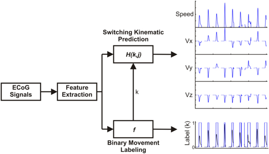
Figure 2. Machine-learning strategy. To predict 3D kinematics, a hierarchical PLS regression model was used. After feature extraction, a logistic regression model classified time windows as either movement or rest. Two PLS regression models were trained, one relating ECoG features and kinematics during movement periods, and a second PLS model relating ECoG features and kinematics during non-movement periods. The final model output was generated from the outputs of the two PLS models by using the logistic regression output to switch between them.
Download figure:
Standard image High-resolution imageThe first component classified whether the patient was moving or not with a logistic regression model using elastic net regularization. A threshold of 10% of the maximum movement speed was applied to generate binary movement and rest labels. The features used to train the model consisted of the z-scores of each of the eight features (seven frequency bands and LMP). To account for potential differences in the optimal time lag between kinematics and neural activity for different channels and features, the Pearson correlation coefficient between training set hand speed and neural activity was calculated with the neural activity leading hand speed at time lags between 0 and 1 s in 50 ms steps. For each channel and feature, the training set data was used to select the lag producing the maximum absolute correlation coefficient with movement speed. To train the logistic regression model, we minimized the loss function shown in equation (1), where X is an n sample ×d feature input matrix of ECoG data, w is a d x 1 weight vector, y is an n x 1 vector of class labels (1 movement, −1 rest), and the  and
and  are the hyperparameter weights associated with the l1 and l2 norms respectively
After finding the set of weights that minimize the loss function above, the output of the model was calculated as shown in equation (2)

The output of the logistic regression model can be considered as a probability that the current time window is from a movement period. Time windows with output probabilities above 0.5 were classified as movement periods and time windows with output probabilities below 0.5 were classified as rest periods. Within the training set, seven fold cross-validation was used to determine the optimal regularization hyperparameters. Finally, the entire training set was used to train the model and the testing set was used to evaluate the accuracy of the model.
The output from this classification step was used to switch between two regression models, one to predict each kinematic parameter while patients were at rest and a second model to predict each kinematic parameter during movement periods. We used a similar method to a prior study that demonstrated the ability to use a PLS regression model to decode continuous traces of kinematic data from ECoG in non-human primates (Chao et al 2010). The PLS model estimates a lower dimensional latent structure and uses this latent structure to fit a regression in order to avoid over-fitting (Wold et al 1984). For our model, the inputs consisted of the z-scored activity for each of the seven canonical frequency bands and the LMP at each channel. Individual feature vectors were produced for time lags between −500 and 1000 ms in 50 ms steps, with positive lags indicating neural activity leading kinematics and negative lags indicating neural activity lagging after kinematics. As the filters used during the preprocessing steps were run both forwards and backwards to avoid phase distortion, the neural activity in each time-window was not necessarily causal relative to the kinematic data, therefore we chose to use neural activity both leading and lagging the kinematic time courses to be predicted. Therefore, the results should be interpreted to represent the entire sensorimotor system and not necessarily causal activity related to motor planning alone. The outputs for the model consisted of movement speed, 3D movement velocity, and 3D hand position. The relationship between ECoG activity and kinematics is described by equation (3), with M(t) representing a kinematic parameter and w representing a prediction weight for a specific channel, feature, and time lag.
Within the training set, we trained models with 1–24 latent features and used seven-fold cross validation to determine the optimal number of latent features that minimized the mean-squared prediction error. The final prediction model was generated from the full training set and the testing set was used to evaluate the accuracy.
2.6.2. Evaluation of prediction accuracy
To evaluate the accuracy of movement prediction, we generated 100 randomly sampled training and testing sets. The accuracy of the classification of movement from rest and of the PLS regression models used to predict kinematics were evaluated independently prior to evaluating the full hierarchical model combining the two models. Accuracy of the classification between movement and rest was calculated as the percent of the total test set windows that were correctly classified. Accuracy of the PLS regression model was evaluated by using the actual movement and rest labels to switch between the two PLS regression models and computing the Pearson correlation coefficient and root mean squared error (rMSE) between the actual and predicted values of each of the 7 kinematic parameters (speed, velocity: Vx, Vy, Vz, and position: X, Y, Z). Finally, the accuracy of the full model was quantified by calculating the Pearson correlation coefficient and rMSE between actual values and predicted values for each of the kinematic parameters.
We evaluated the statistical significance of the models using two surrogate methods to ensure that accurate predictions were generated from the specific patterns of ECoG activity and not from any systematic bias. First, we generated a surrogate kinematic dataset by randomly reordering the trials within the training set, randomly selecting a new trial onset from within each training set trial, and generating a new time course by wrapping data from the beginning of the trial to the end of the trial. This procedure ensured that the temporal relationship between the ECoG signals and kinematics was random, while maintaining the autocorrelation structure of the kinematics. The binary movement labels and continuous kinematic traces were reshuffled in the same fashion, so any differences between actual and surrogate predictions were not driven by the ability to decode movement and rest periods. For each training and testing set, we trained one model using the original kinematic data and a second model using the surrogate kinematics. Both models were tested using the original testing set. A second surrogate method that was similar to one used in other studies of kinematic prediction (Chao et al 2010, Hotson et al 2014) was also used to randomly vary ECoG features and channel assignments. For each training set, we reshuffled the channel and frequency assignments of the prediction weights 100 times and generated test accuracies using both the original and reshuffled weights. The statistical significance of both the movement classification and kinematic prediction models was evaluated using a Wilcoxon rank sum test to compare the median actual accuracy with the median surrogate accuracy. Bonferroni correction was used to correct for the total number of predictions (five patients × seven kinematic variables × two surrogate methods).
2.6.3. Computation of movement trajectories
To determine the optimal method for generating movement trajectories, we compared the accuracy of the original position predictions with position predictions generated by concatenating the predicted velocity vectors. The overall accuracy was then quantified by determining the percent of trials in which the actual and predicted trajectories ended in the same quadrant.
2.6.4. Evaluation of feature importance
Because the z-score operation equalized the variance of each feature prior to generating prediction models, the weights for each channel and feature could be compared to evaluate the importance of each feature type and electrode location. While the PLS model weights represent the optimal combination of ECoG signals to decode kinematics, they do not necessarily represent the strength of the relationship between movement kinematics and ECoG data (Haufe et al 2014). Therefore, the decoding model weights were converted to activation patterns describing the encoding of kinematics by ECoG signals (equation (4)) (Haufe et al 2014), where W represents the matrix of prediction weights, ΣX represents the ECoG covariance matrix, ΣS represents the kinematic data covariance, and A represents the activation patterns.

To examine the importance of features in the classification of movement and rest conditions, logistic regression prediction weights were averaged across each of the 100 training sets. For each frequency band, the magnitude and location of average model weights was mapped onto an atlas brain using a weighted spherical Gaussian kernel (full-width at half-max: 9.2 mm) centered at each electrode location. In patients with overlapping electrode coverage, Gaussian kernels were combined using a weighted average based upon the distance from each electrode. For the PLS regression model predicting movement period kinematics, the relative importance the absolute value of the prediction weights and activation patterns for a given channel, feature, and lag were normalized by the sum of the absolute value of all prediction weights or activation patterns as shown in equation (5)
Normalized weights and activation patterns were calculated for each channel by summing the across features and time lags (equation (6)). Normalized channel weights and activation patterns were mapped onto a single atlas brain to evaluate the importance of cortical locations within the model

The importance of the eight ECoG feature types used in the PLS model was evaluated in two ways. First the maximum PLS weight and activation pattern at each frequency was determined. Second, after identifying the 1% of model weights and activation patterns with the highest absolute values, the percentage of these weights in each frequency was calculated. The two methods identified features that had a large impact on PLS predictions either because of weights with very high values or a large number of moderately large weights.
2.6.5. Asynchronous kinematic prediction
To determine whether the proposed model can be applied to an asynchronous dataset, an additional model was trained for patient 5. After removing trials with artifacts, all remaining data including movement, rest, and ITI periods were used. Training and testing sets were generated using eight-fold cross validation with each testing set drawn from consecutive trials. The logistic regression and PLS regression models were calculated from the training sets as described in section 2.6.1 and evaluated on the test sets.
3. Results
3.1. Behavioral performance
All patients were able to consistently and accurately perform reaching movements to the target locations with no differences in movement times between targets. To evaluate the true dimensionality of the reaching movements performed, the percent of variance explained by the principle components of the seven kinematic parameters used: speed, velocity (Vx, Vy, Vz), and position (X, Y, Z) is shown in table 2. The first principle component explained at most 35% of the variance and each of the first four principle components explained at least 11% of the variance. Additionally, the average cross-correlation between kinematic parameters (table 3) shows that, as expected for a center-out reaching task, while each directional component of velocity is positively correlated with its respective position, speed is not correlated with any direction and there are no cross-directional correlations.
Table 2. Variance explained by principal components of kinematics.
| Principal component variance | |||||||
|---|---|---|---|---|---|---|---|
| Patient | PCA 1 | PCA 2 | PCA 3 | PCA 4 | PCA 5 | PCA 6 | PCA 7 |
| 1 | 22% | 19% | 17% | 14% | 11% | 10% | 6% |
| 2 | 26% | 22% | 19% | 13% | 9% | 6% | 5% |
| 3 | 35% | 21% | 18% | 11% | 7% | 5% | 3% |
| 4 | 24% | 23% | 16% | 13% | 11% | 8% | 5% |
| 5 | 24% | 22% | 20% | 14% | 8% | 7% | 6% |
Table 3. Average cross-correlation of kinematics.
| Speed | Vx | Vy | Vz | X Position | Y Position | Z Position | |
|---|---|---|---|---|---|---|---|
| Speed | 1.00 | 0.00 | −0.06 | 0.01 | 0.12 | 0.00 | −0.07 |
| Vx | 0.00 | 1.00 | 0.12 | −0.21 | 0.43 | 0.01 | −0.05 |
| Vy | −0.06 | 0.12 | 1.00 | −0.05 | −0.03 | 0.52 | 0.06 |
| Vz | 0.01 | −0.21 | −0.05 | 1.00 | −0.03 | 0.00 | 0.47 |
| X Position | 0.12 | 0.43 | −0.03 | −0.03 | 1.00 | 0.08 | −0.21 |
| Y Position | 0.00 | 0.01 | 0.52 | 0.00 | 0.08 | 1.00 | −0.02 |
| Z Position | −0.07 | −0.05 | 0.06 | 0.47 | −0.21 | −0.02 | 1.00 |
3.2. Classification of movement and rest
The first level of the decoding model was a logistic regression to classify each time point as movement or rest. While the ability to classify movement and rest periods using ECoG is not novel in itself, it is important to demonstrate as the first component of the hierarchical decoding model used. Exemplar binary predictions of movement and rest are shown for a test set from a single patient in figure 3. The predicted movement states match the actual labels closely, showing a good ability to predict whether a patient is moving or not using ECoG. Accuracies of predictions of movement and rest are shown in table 4. Final prediction accuracies were compared to chance prediction levels produced with two surrogate datasets derived by shuffling the temporal relationship between movement class labels and ECoG data, or by shuffling the channel and feature assignments of the model weights. Supplementary figure S1 shows exemplar surrogate predictions for a single patient. The true prediction accuracy is significantly higher than accuracy produced by either of the surrogate datasets in all patients after Bonferroni correction for the total number of comparisons. Because the movement and rest classes were unbalanced, prediction accuracies produced by the surrogate methods were similar to the overall proportion of movement and rest classes in the dataset. This can be seen in figure S1 as the surrogate models classify the majority of windows as rest.
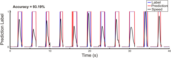
Figure 3. Exemplar classification of movement and rest periods. Exemplar predictions of movement classes were generated using consecutive trials within a single held-out test set from Patient 5. Black traces show the actual hand speed that was used to generate true movement class labels shown in blue. Predicted movement class labels are shown in red and correspond well with the actual labels.
Download figure:
Standard image High-resolution imageTable 4. Accuracy of classification of movement and rest. Accuracies show mean (st. dev.) of the percent of windows predicted correctly.
| Patient | Original accuracy | Shuffled time accuracy | p | Shuffled feature accuracy | p |
|---|---|---|---|---|---|
| 1 | 67.78% (2.02) | 53.28% (1.97) | <0.000 001 | 50.92% (3.40) | <0.000 001 |
| 2 | 73.43% (3.93) | 48.91% (5.59) | <0.000 001 | 50.08% (4.96) | <0.000 001 |
| 3 | 81.97% (3.23) | 63.42% (2.28) | <0.000 001 | 60.82% (3.75) | <0.000 001 |
| 4 | 85.08% (2.40) | 60.22% (2.64) | <0.000 001 | 56.06% (4.40) | <0.000 001 |
| 5 | 90.10% (1.36) | 70.97% (1.42) | <0.000 001 | 69.57% (2.18) | <0.000 001 |
3.3. Continuous kinematic prediction
The second level of our machine learning model was composed of two PLS regressions, one to describe the relationship between ECoG features and speed, velocity, and position during non-movement periods, and a second model to characterize the relationship between ECoG signals and kinematics during movement periods. To examine the ability of this hierarchical PLS regression model to predict the time courses of kinematics during novel time periods, we trained each of the PLS regression models on a training set and used a separate test set to evaluate the prediction accuracy. We first evaluated the ideal performance of the PLS regression in isolation from the movement classification and later evaluated the combined model accuracy.
3.3.1. PLS regression model
To evaluate the accuracy of the PLS regression model alone, actual movement and rest labels were used to switch between the PLS regressions. PLS model predictions of movement speed were significantly more correlated with actual hand speed than either of the surrogate models in all patients as shown in figure 4. Predictions of movement speed also had significantly lower rMSE values than either surrogate model. Because both the real and surrogate models were trained with speed amplitudes that were high during the movement model training data and low during the rest model training data, speed predictions are higher in the movement period for both actual and surrogate predictions. However, as can be observed in figure S2, the shape of speed predictions is significantly worse for both surrogate methods. Ideal test accuracies across patients are shown in figure 4 for velocity and position. The PLS model accuracy for both directional and non-directional kinematic variables are summarized in table 5. Predictions of velocity had significantly greater correlations and significantly lower rMSE values than both surrogate models for 12 of the 15 velocity components (three directions, five patients). Position predictions had significantly greater correlation coefficients and significantly lower rMSE values when compared to both surrogate models in 10 of 15 position components tested. Therefore, components of 3D kinematics were predicted by our hierarchical PLS model with accuracies better than chance in multiple patients. While the ability to predict movement and rest periods well may influence the size of the correlation values, the surrogate movement and rest models also differentiated movement and rest periods as can be seen in figure S2. Additionally, because movements were made in both directions, predicting movement and rest cannot solely account for the positive correlation values that were observed. Significant statistical differences between actual and surrogate model predictions were also found from the movement period alone (table S1). Therefore, the significant differences between actual and surrogate prediction accuracies were not caused by the difference between movement and rest but because the PLS regression models allowed us to predict kinematics with accuracies better than chance.
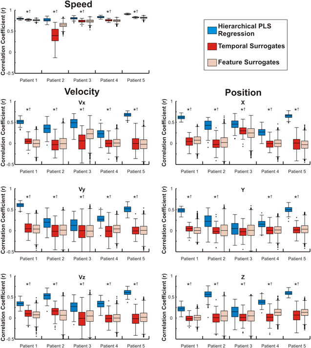
Figure 4. Movement kinematics are predicted with accuracies better than chance. Distributions show the correlation coefficients (Pearson's r) between predicted and actual movement kinematics generated using the hierarchical PLS regression model. Distributions were generated from test sets using the actual movement class labels to switch between the PLS regression models. Boxes represent the median, 25th, and 75th percentiles and whiskers extend to the most extreme data points with outliers greater than 2.7 standard deviations marked with a +. *—Distributions with significantly higher correlations than the surrogate model generated by shuffling the temporal relationship between ECoG and kinematics, †—Distributions with significantly higher correlations than the surrogate model generated by shuffling feature and channel weights.
Download figure:
Standard image High-resolution imageTable 5. PLS model prediction accuracies. Median accuracies, Pearson's r and rMSE, between predicted and actual kinematics. Predictions were generated using the actual movement labels to switch between PLS models, isolating the PLS regression model from the movement classification.
| Correlation | |||||||
|---|---|---|---|---|---|---|---|
| Velocity | Position | ||||||
| Patient | Speed | Vx | Vy | Vz | X | Y | Z |
| 1 | 0.7936a b | 0.5156a b | 0.6125a b | 0.345a b | 0.6201a b | 0.4906a b | 0.2171a b |
| 2 | 0.7664a b | 0.3521a b | 0.2015a b | 0.5349a b | 0.4285a b | 0.2238a b | 0.5620a b |
| 3 | 0.8084a b | 0.4908a b | 0.1273a b | 0.2756a b | 0.4564a b | 0.0507 | 0.1509a b |
| 4 | 0.8341a b | 0.2285a b | 0.2725a b | 0.3451a b | 0.2702a b | 0.1544a b | 0.3800a b |
| 5 | 0.9072a b | 0.6796a b | 0.5207a b | 0.6076a b | 0.6575a b | 0.5004a b | 0.5928a b |
| Root mean-square error | |||||||
| Velocity | Position | ||||||
| Patient | Speed (cm s−1) | Vx (cm s−1) | Vy (cm s−1) | Vz (cm s−1) | X (cm) | Y (cm) | Z (cm) |
| 1 | 10.26a b | 11.39a b | 9.52a b | 11.25a b | 7.11a b | 7.9a b | 8.42b |
| 2 | 8.6a b | 8.19a b | 10.35a | 9.39a b | 7.03a b | 9.66b | 7.43a b |
| 3 | 8.86a b | 8.47a b | 11.05 | 9.31a b | 5.86a b | 8.52 | 6.89 |
| 4 | 8.81a b | 10.87b | 10.99a b | 10.32a b | 7.35a b | 8.48 | 8.43a b |
| 5 | 9.22a b | 10.59a b | 12.43a b | 11.04a b | 6.59a b | 7.84a b | 6.68a b |
aSiginificantly different from a surrogate model created using temporally reshuffled training data. bSignificantly different from a surrogate distribution created by reshuffling channel and feature weights.
3.3.2. Full regression model
Median correlations between actual and predicted kinematics are shown in table 6 for the full model predictions using both the logistic regression and PLS regression models. Accuracies for the full model prediction are lower than when actual movement labels are used to switch between PLS regression models (table 5). Additionally, velocity and position accuracies are highest along the x (anterior–posterior) axis and lowest along the y (lateral) axis. When using the predicted movement classes to switch between PLS regression models, predictions of speed were significantly more correlated to the actual movement speed and had significantly lower rMSE values than both surrogate methods in four of the five patients. Predictions of velocity components had significantly greater correlations and significantly lower rMSE than both surrogate models for 11 of 15 velocity components and position predictions had significantly greater correlations and significantly lower rMSE than both surrogate models for 9 of 15 position components. Exemplar time courses of actual and predicted kinematics using the full hierarchical PLS regression model are shown for a single patient in figure 5. As can be seen, time courses of predicted kinematics align well with the time courses of actual reaches.
Table 6. Full model prediction accuracies. Median accuracies, measured with Pearson's r and rMSE between predicted and actual kinematics. Predictions were generated using the full hierarchical model.
| Correlation | |||||||
|---|---|---|---|---|---|---|---|
| Velocity | Position | ||||||
| Patient | Speed | Vx | Vy | Vz | X | Y | Z |
| 1 | 0.3144 | 0.3692a b | 0.4455a b | 0.1679a b | 0.5605a b | 0.4497a b | 0.1624a b |
| 2 | 0.5881a b | 0.3009a b | 0.2002a b | 0.4686a b | 0.3934a b | 0.204a b | 0.5588a b |
| 3 | 0.6564a b | 0.4267a b | 0.1481a b | 0.2397a b | 0.4171a b | 0.0696 | 0.1764a b |
| 4 | 0.749a b | 0.2181a b | 0.2518a b | 0.3346a b | 0.2543a b | 0.1504a b | 0.3685a b |
| 5 | 0.7961a b | 0.6302a b | 0.4437a b | 0.55a b | 0.6579a b | 0.5128a b | 0.5486a b |
| Root mean-square error | |||||||
| Velocity | Position | ||||||
| Patient | Speed | Vx (cm s−1) | Vy (cm s−1) | Vz (cm s−1) | X (cm) | Y (cm) | Z (cm) |
| 1 | 18.16 | 12.62a b | 10.99a b | 12.13b | 7.50a b | 8.07a b | 8.62b |
| 2 | 11.20a b | 8.44a b | 10.44 | 9.85a b | 7.27a b | 9.64b | 7.48a b |
| 3 | 11.32a b | 8.70a b | 10.91 | 9.51a b | 5.96b | 8.34 | 6.81 |
| 4 | 10.64a b | 10.92b | 11.09a b | 10.26a b | 7.41a b | 8.45 | 8.45a b |
| 5 | 13.30a b | 11.19a b | 12.97a b | 11.52a b | 6.55a b | 7.74a b | 6.96a b |
aSiginificantly different from a surrogate model created using temporally reshuffled training data. bSignificantly different from a surrogate distribution created by reshuffling channel and feature weights.
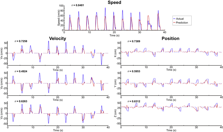
Figure 5. Exemplar kinematic predictions. Full model predictions were generated using the predicted movement classes from the logistic regression to switch between PLS model outputs. Actual kinematic traces are shown in blue and predicted traces are shown in red. Predictions in each plot were generated from consecutive trials from a single test set from patient 5.
Download figure:
Standard image High-resolution imageBecause position predictions made by concatenating predicted velocity vectors were more accurate than the original PLS model position predictions, this method was used to compute trajectories for each trial. The accuracy of the full model was quantified by determining the percentage of trials in which the actual and predicted movement trajectories ended in the same quadrant. The final accuracy of target predictions was 49.0%, 44.5%, 45.1%, 40.0%, and 66.2% for patients 1–5 respectively, each of which is higher than the 12.5% accuracy expected by chance. The predicted trajectories were finally averaged for each of the eight target classes after normalizing the trial time course. Exemplar average movement trajectories are shown for a single patient in figure 6 demonstrating that movements were predicted accurately in each direction.
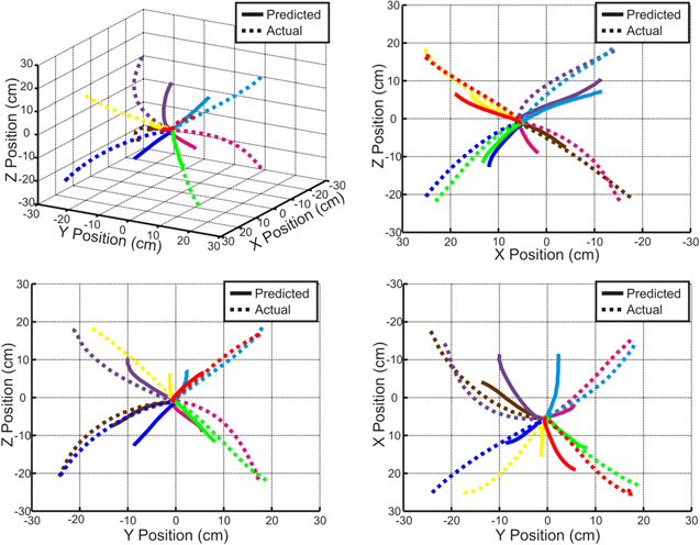
Figure 6. Average predicted trajectories. Average actual and predicted trajectories from Patient 5 are shown for each of the eight targets. Predicted trajectories were generated by concatenating predicted velocity vectors obtained from the full model and were then averaged for each target. Correlation coefficients (Pearson's r) between the actual and predicted movement trajectories for the eight targets range from 0.86 to 0.99.
Download figure:
Standard image High-resolution image3.4. Feature importance
We sought to evaluate the importance of individual ECoG feature types and cortical locations. Average model weights for the logistic regression model used to classify movement and rest periods across patients are shown for selected features in figure 7. Beta band and LMP features, in particular, demonstrate the largest amplitude prediction weights with negative weights centered in primary sensorimotor areas, indicating that decreases in sensorimotor cortex beta band power and LMP amplitude are associated with movement periods. The lags for the largest amplitude weights were between 0 and 150 ms with neural activity leading the prediction.

Figure 7. Logistic regression model weights for movement and rest classification. Average logistic regression model weights are shown for selected frequencies. Beta band power and LMP amplitude in primary sensorimotor cortices have the strongest prediction weights across patients with decreases in beta band power and LMP amplitude associated with movement periods. Regions shown in dark gray had no electrode coverage.
Download figure:
Standard image High-resolution imageTo evaluate the importance of individual features and cortical regions for the prediction of continuous kinematic parameters, we examined the movement period PLS regression models. In addition to the decoding model weights, activation patterns were calculated to examine kinematic encoding at each location and are plotted in figure 8. While the largest weights were located over sensorimotor regions, large amplitude weights are also observed from diffuse regions of cortex. In contrast, the activation patterns are much better localized to sensorimotor regions with a clear peak in the superior motor cortex. While each dimension (X, Y, and Z) was predicted well, at the current electrode size, no cortical representation of directionality was observed. Across temporal and spectral features, the maximum normalized weight amplitude and percent of the largest 1% of prediction weights demonstrated similar trends (figure 9). In particular, LMP and high gamma features in the 65–95 Hz and 130–175 Hz ranges represented the most important prediction weight features. For the activation patterns, strong encoding of kinematics was observed for the LMP, mu band, beta 1 band, and high gamma bands. Additionally, while both causal and non-causal temporal lags were considered, the peak activation patterns were observed at lags between 250 and 400 ms with neural activity leading the predicted kinematics.
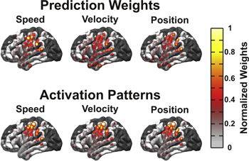
Figure 8. Topography of PLS prediction weights. Absolute values for movement-class PLS regression weights and activation patterns compared across cortical locations for all patients. The color scale represents the normalized absolute value of prediction weights and activation patterns by cortical location. While prediction weights are spread over diffuse regions of cortex, activation patterns show that kinematics are encoded most strongly in sensorimotor areas. Regions shown in dark gray represent regions with no electrode coverage.
Download figure:
Standard image High-resolution image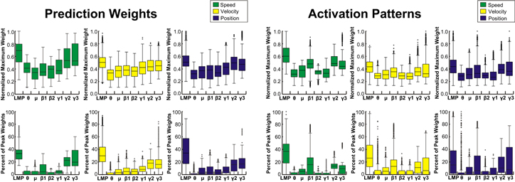
Figure 9. Importance of ECoG feature types for kinematic prediction. Distributions represent the maximum absolute movement-class PLS prediction weights and activation patterns for each feature and the percentage of the highest 1% of weights from each feature across patients and electrodes. LMP and high gamma band features have the largest prediction weights, while activation patterns demonstrate that LMP, mu, beta, and high gamma bands all encode kinematics.
Download figure:
Standard image High-resolution image3.5. Asynchronous prediction of kinematics
To simulate on-line BCI performance, a model was trained for patient 5 without time-locking to individual trials. Patient 5 was chosen because this patient had the most accurate time-locked predictions (table 6). Figure 10 shows an exemplar period of this pseudo real-time, continuous prediction spanning several consecutive trials. A video demonstrating trajectory predictions made by concatenating the predicted velocity vectors is included in the on-line supplemental materials.

Figure 10. Exemplar asynchronous prediction: Asynchronous predictions were made by training a model using all time points (including movement trials and ITI periods). The plots show 50 s of consecutive actual and predicted kinematics from a single test fold, demonstrating that the method presented has the potential to be applied in real-time BCI applications.
Download figure:
Standard image High-resolution image
4. Discussion
This study demonstrates that kinematic parameters, in particular speed, velocity, and position, of 3D reaching movements can be decoded from ECoG signals in human patients. The ability to decode kinematics of reaching movements with several degrees of freedom builds upon previous demonstrations that ECoG signals can be used to decode movement trajectories (Schalk et al 2007, Pistohl et al 2008, Sanchez et al 2008, Ganguly et al 2009, Chao et al 2010, Shimoda et al 2012, Marathe and Taylor 2013) and to control closed-loop BCIs (Leuthardt et al 2004, Wilson et al 2006, Felton et al 2007, Schalk et al 2008, Rouse and Moran 2009, Rouse et al 2013). Although a few previous studies have decoded movement trajectories from movements that were not constrained to two dimensions (Hotson et al 2012, Chen et al 2013, Hotson et al 2014), the movements used were correlated with speed in at least one dimension, reducing the dimensionality of the movements. In the task used in this study, the first kinematic principle component explained at most 35% of the variance in any patient and the first four principle components each explained at least 11% of the variance in all patients, indicating that the movements performed and decoded included multiple independent dimensions. Therefore, we believe that this study provides the first true demonstration of the ability to use ECoG recordings from human patients to decode 3D kinematics. While 3D kinematic decoding has also been demonstrated from ECoG recordings in non-human primates (Chao et al 2010, Shimoda et al 2012), the demonstration of kinematic decoding in humans substantially adds to these findings. Non-human primates typically require extensive periods of behavioral training prior to the recording of neural activity, leading to more consistent motor movements than would be expected in real-world behavior. Additionally, as long-term practice of a motor task leads to an increase in the size of the cortical area activated during task performance (Karni et al 1995), decoding of behavioral intentions during a trained motor task may not generalize to more typical novel behaviors.
In addition to spectral power changes, the LMP signal was striking for the strength of its PLS model weights and activation patterns. As the LMP is derived from low-pass filtering ECoG signals, it is likely that there is a correspondence to movement-related cortical potentials such as the bereitschaft potential that are characterized by a negative shift in signal amplitude with an increasing negativity immediately before the movement onset (Kornhuber and Deecke 1965, Deecke et al 1969, Shibasaki and Hallett 2006). Similarly, the LMP signal was negatively correlated with movement speed in sensorimotor regions. A number of previous studies have shown that LMP amplitude can be used to decode position and velocity during arm movements (Schalk et al 2007, Pistohl et al 2008, Ganguly et al 2009, Hotson et al 2014), therefore the large amplitude of prediction weights and activation patterns is unsurprising.
In designing our hierarchical PLS regression model, we chose to use the logistic regression and PLS regression methods in part because they are both linear. Therefore, as the ECoG features were transformed to z-score values prior to training the prediction model, we were able to easily interpret and compare the importance of each cortical location and feature. As the prediction accuracy was improved when real movement and rest labels were used, future work could improve the model accuracy either by improving the classification of movement and rest, or through improving the kinematic decoding. Potential methods to improve decoding accuracy include: calculating spatial filters through unsupervised methods such as independent component analysis (Makeig et al 1996, Kachenoura et al 2008), supervised learning methods such as common spatial patterns (Koles et al 1990, Koles 1991, Ramoser et al 2000, Blankertz et al 2008, Ince et al 2010, Marathe and Taylor 2013), using a model such as a kalman filter that incorporates temporal filtering into the prediction model (Wu et al 2003, Marathe and Taylor 2013), or by using an alternative linear or nonlinear machine learning method (Wessberg et al 2000). It should be noted that these alternative methods are not guaranteed to increase prediction accuracies as they may be poorly suited to fit the relationship between ECoG activity and movement kinematics. Additionally, although several variants of the common spatial patterns algorithm have been designed to reduce overfitting (Blankertz et al 2008, Foldes and Taylor 2011, Lotte and Guan 2011, Falzon et al 2012, Samek et al 2012), these algorithms may still be susceptible to overfitting due to the large feature space and limited amount of training data available. Along with speed, velocity, and position, there are a number of other movement parameters that describe movements such as joint angles or muscle activations. One factor in choosing to begin by decoding speed, velocity, and position is their prevalence in prior studies of single-unit motor control (Georgopoulos et al 1982, Moran and Schwartz 1999, Wang et al 2007) and movement decoding with ECoG (Schalk et al 2007, Pistohl et al 2008, Ganguly et al 2009, Chao et al 2010, Marathe and Taylor 2013). While we have shown that speed, position, and velocity can be decoded from ECoG recordings in human patients, algorithms designed to decode alternative components of reaching movements may lead to increases in the accuracies of decoded trajectories.
Along with alternative decoding algorithms, the ability to decode movement kinematics would likely be improved by optimizing the ECoG implants. As the ECoG arrays were implanted for clinical purposes, the location, size, and extent of electrode coverage were all based upon clinical necessity. Recently, it has been found that ECoG electrodes with smaller sizes and spacing can be used to examine neural activity with increased spatial resolution (Leuthardt et al 2009, Wang et al 2009, Kellis et al 2010). Additionally, as the arrays used here missed the most superior portions of the motor cortex, optimizing implant locations for decoding neural activity through the use of pre-operative functional imaging techniques (Wang et al 2013) would likely improve decoding accuracy. Taken together, we believe the level of accuracy in this study represents a lower bound that can be improved upon by future studies optimizing electrode arrays and implant locations for BCI systems in patient populations. While these clinical electrode implants required large craniotomies and were highly invasive, future generations of BCI-specific ECoG arrays are likely to substantially reduce the invasiveness of implant procedures (Schalk and Leuthardt 2011).
This study shows that arm movement kinematics have broad cortical representations that can be recorded with ECoG electrode arrays. There are several potential alternative considerations that should be noted. First, due to the margin of error in localizing electrodes onto cortex and intersubject variability in neural anatomy, there is some variance inherent in the localization of decoder weights onto an atlas brain. Next, all of the recordings were made in chronic epilepsy patients. Although care was taken to ensure that all seizures occurred at least 2 h before or after recordings were made, and that trials with interictal activity were removed prior to analysis, it is difficult to determine if the results of this study were affected by the patient population used. As 4 of the 5 patients had epileptic foci located in the temporal lobe away from sensorimotor areas, we believe that the results were not significantly affected by focal epileptic activity. Additionally, as the reaches used involved the entire arm, it is uncertain if these results will generalize to isolated movements of more distal body parts. Because of this, the results of this study must be interpreted within the context of the activity of the entire motor system and not of individual musculature. Regardless of the role of stabilizing movements, the fact that we can decode information with multiple degrees of freedom still demonstrates the potential for BCI system development. Our decoding model used neural activity both leading and lagging kinematic movements, which would not be possible in a causal BCI system, however, the ability to use ECoG signals to decode movement kinematics underscores the degree of information that can be decoded from ECoG activity, representing a significant step towards the development of ECoG BCI applications. Finally, the broad distribution of decoder weights may function either to amplify movement-related neural activity or to remove non-movement related covariant activity. The activation patterns, representing the features with the strongest relationship with kinematics, were more localized to sensorimotor regions with a clear peak in the more superior areas of motor cortex as expected.
While we have shown that ECoG signals from human patients can be used to decode kinematics of 3D reaches, the optimal method to evaluate the accuracy of a BCI system is ultimately through closed-loop experiments. Open-loop decoding of motor activity allows us to assess the feasibility of BCI algorithms, but there are a number of important differences between open-loop and closed-loop methods. In particular, closed-loop BCI control provides feedback to the user, allowing them to learn to adapt their neural activity to improve the accuracy of the BCI system (Taylor et al 2002, Jarosiewicz et al 2008, Rouse and Moran 2009, Rouse et al 2013). Additionally, co-adaptively modifying the decoding model in conjunction with the subject's ability to learn has led to further improvements in on-line BCI control (Williams 2013), indicating that the open-loop accuracies demonstrated in this work could be further improved upon during closed-loop BCI control. Because decoding accuracy can improve though closed-loop adaptation, BCI systems should be designed to enhance the ability of the BCI user to learn and adapt. For example, although open-loop decoding accuracies can be maximized by using algorithms with slow temporal update times, closed-loop decoding accuracies are maximized by algorithms with fast temporal updates allowing for better on-line adaptation (Cunningham et al 2011). Therefore, it will be important for future studies to 'close the loop' in order to ensure that algorithms that increase the accuracy of off-line kinematic decoding will also have corresponding increases in BCI control performance. A further question is how valuable the LMP will be for closed-loop control. In line with previous studies (Schalk et al 2007, Pistohl et al 2008, Hotson et al 2014), we found that the LMP amplitude had a significant contribution to the decoding of kinematics. Although the LMP signal is clearly important for movement decoding, very few studies have used time domain signals for BCI control (Kennedy et al 2004a, 2004b). Because the LMP is derived from low-pass filtering ECoG signals, it changes on a relatively slow time scale. This slow time scale may make it difficult for patients to adapt their LMP signals during BCI control. Future studies using LMP signals within closed-loop BCI systems will be important to understand the advantages and disadvantages of the LMP signal for BCI control.
Taken together, the results of this study provide an exciting demonstration of the ability to use ECoG recordings to decode 3D kinematics of reaching movements in human patients. This underscores the potential to utilize ECoG to develop BCI systems with multiple degrees of freedom for translation into multiple patient populations.
Disclosures
ECL has stock ownership in the company Neurolutions. DTB has received consulting fees from the company Neurolutions.
Acknowledgments
This publication was supported by the James S McDonnell Foundation and the Washington University Institute of Clinical and Translational Sciences grants UL1 TR000448 and TL1 TR000449 from the National Center for Advancing Translational Sciences.