LOCUST-GPU predictions of fast-ion transport and power loads due to ELM-control coils in ITER

S.H. Ward; R. Akers; L. Li; Y.Q. Liu; A. Loarte; S.D. Pinches; A. R. Polevoi; R.G.L. Vann; M.A. Van Zeeland

doi:10.1088/1741-4326/ac904f

1. Introduction

The ITER tokamak aims to operate in high-confinement mode (H-mode) [1] to achieve high-gain (Q ∼ 10), stationary ( $\sim 500$ s) plasma discharges [2]. However, the additional power expelled during the type-I edge-localised modes (ELM) typically observed in H-mode plasmas poses a risk to plasma performance and can significantly reduce the lifetime of plasma-facing components (PFC), limiting the operational availability of ITER-scale devices [3]. To mitigate or suppress ELMs, ITER is equipped with a set of ELM-control coils (ECCs) that impose resonant magnetic perturbations (RMP) onto the plasma, breaking the underlying tokamak equilibrium axisymmetry.

Experimental and computational studies have suggested that RMPs lead to increased transport of fast ions [4]. Particles are predicted to be mostly affected where the RMP amplitude is greatest, often at the edge of the plasma, where the neutral beam injection (NBI) deposits part of its intense, anisotropic source of fast ions. Hence many studies corroborate the impact that the application of ECCs has on NBI ions in particular—specifically, the resulting reduction in beam ion confinement, NBI heating efficiency and associated increase in power flux to PFCs. All of these impacts must be mitigated if ITER is to achieve its aims.

The distribution of the PFC power flux is thought to be dictated by the influence on fast-ion orbits by the various magnetic structures that exist within the RMP field [5–9]. These structures are influenced in turn by the design and operation of the ECCs [10]—that is, the geometry of each coil and current it carries—in combination with the plasma's response to the externally imposed RMP field [11, 12], which may reduce [13] or amplify the RMP field [4] and resulting transport [12]. Therefore, the potential impact that ITER's high-power NBI system (a 33 MW flux of 1 MeV deuterons in the initial baseline configuration [14]) poses to the power loads on PFCs [15] (designed to tolerate up to 10 MW m⁻² maximum at the divertor, less elsewhere [16]) could be aggravated or mitigated depending on how the ECC system is operated. This potential optimisation is why the ongoing study of ECC operation, plasma response models, and their combined influence on the PFC power flux is necessary to support the refinement of the ITER research plan [2].

Despite the importance of this topic, it remains challenging to study computationally due to the extreme scale of the ITER device. Kinetic fast-ion codes which aim at accurately resolving PFC power loads must cope with a huge spatiotemporal domain (1 s slowing down time, $\sim 800\enspace {\text{m}}^{3}$ plasma volume), model expansive yet intricate wall geometries, and resolve fine structures in RMP fields. This bottlenecks attempts to systematically simulate the ITER system without significant computational resources, making the optimisation problem difficult. However, the Lorentz-orbit code for use in stellarators and tokamaks (LOCUST) code [17] is a novel kinetic fast-ion algorithm that is designed to make reactor-scale systems tractable on desktop hardware. While this could potentially provide a way of discovering new physics, in this context LOCUST also enables the routine study of ITER at high fidelity, allowing for precise optimisation—for example through the minimisation of localised, component-specific power loads.

This paper aims to evaluate methods of mitigating reductions in NBI heating efficiency and localised PFC power loads due to ECCs by predicting the related fast-ion transport in ITER. The distribution of lost NBI power is calculated for applied n₀ = 3 and n₀ = 4 ECC waveforms, which can be oscillated to rotate the RMP toroidally while maintaining ELM suppression. Here, n₀ is used to indicate the fundamental toroidal mode number of the applied perturbation. To resolve the PFC power at the component level, we use the LOCUST code to model fast-ion dynamics in the presence of detailed and realistic models of the first wall and RMP field. Because of this, we have also verified the implementation and convergence of the 3D magnetic field model in LOCUST.

After describing and testing the 3D magnetic field model in section 2, the ITER ECC system, and the physical model used to represent it, is described in section 3. Section 4 then presents the results of studying this model with LOCUST, including the measured fast-ion transport and PFC power loads at different RMP phases. Finally, section 5 presents a summary and outlook of the work.

2. 3D magnetic fields in `LOCUST`

LOCUST is a high-performance kinetic fast-ion code. It utilises hardware acceleration via programmable graphics processing units (GPU) and tuned software algorithms to massively parallelise the calculation of fast-ion slowing-down trajectories at speeds unobtainable with traditional central processing unit (CPU) codes. LOCUST achieves this by assigning fast-ion markers to individual GPU threads, which each solve the particle Lorentz equation of motion and periodically apply a Fokker–Planck collision operator. This allows for the efficient, full-orbit tracking of large populations (millions) of markers over long periods of time (seconds). For this reason, the code is uniquely suited for calculating fast-ion transport and detailed PFC power loads in ITER.

To ensure accuracy when extrapolating to ITER, we tested the implementation of 3D magnetic fields in LOCUST by applying it to an already operating device where the impact of RMPs on NBI fast-ion confinement has been assessed experimentally and by other modelling tools. The code has previously been shown [17] to compare well with other fast-ion codes and experiment in a variety of scenarios with axisymmetric plasmas, including those with ITER-similar shapes such as DIII-D shot #157418 [7]. Here we study DIII-D shot #157418 again, including the n₀ = 3 RMP applied during the discharge.

Using the same plasma input data from [7], the corresponding results from LOCUST were compared to the simulations presented in [7] by SPIRAL [18]. SPIRAL is a widely accepted code that is regularly used in comparisons with experiment. Though SPIRAL's speed and reliance on conventional CPU hardware makes it unable to study ITER at high fidelity without significant computational resources, its wide use makes the code very well-suited for verification exercises. LOCUST used a higher precision version of the perturbed field and plasma response calculated by M3D-C1 [19], generated on a grid with 3.7 mm spacing to ensure convergence. LOCUST used the same neutral beam deposition as SPIRAL, which was generated by beams injected both co and counter to the plasma current, including all three energy components as well as the effects of the plasma displacement on the temperature and density profiles due to the applied RMP.

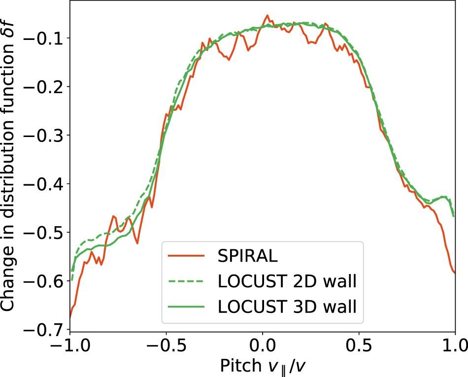
Figures 1 and 2 show the changes in the steady-state fast-ion distribution function, f, caused by the RMP. The distribution function is cropped to include only the plasma edge, in regions satisfying ρ > 0.77, where ρ represents the square root of the normalised toroidal flux. Though this cut-off is different in [7], where ρ > 0.7, the small volume within 0.7 < ρ < 0.77, and the resulting influence of finite bin-widths, means manual tuning was required to capture this sensitive region. Figure 1 shows the difference between f calculated with and without the 3D magnetic field, f_3D(, λ) − f_2D(, λ), as a function of energy and particle pitch angle λ = v_||/v measured against the plasma current. There is good qualitative agreement between the codes; both show transport in the same region of phase space, corresponding to edge-localised, co-passing particles. Of these particles, those with energies above 40 keV—half injection energy—are affected somewhat differently between the simulations. Figure 2 illustrates this more clearly, showing the RMP-induced transport as a fraction of the axisymmetric distribution function, $\left[{f}_{3\text{D}}(\lambda )-{f}_{2\text{D}}(\lambda )\right]/{f}_{2\text{D}}(\lambda )$ . The effect of these high-energy markers is a 10% point difference in the transport within 0.8 < λ < 1.0, > 40 keV. This could be because SPIRAL, unlike LOCUST, extends the electron density profile past the last-closed flux surface, generating increased drag at higher energies for edge-localised markers. Likewise, LOCUST did not include plasma rotation, impurities or electric fields. Both 2D and 3D representations of the first wall were used in LOCUST to gauge the effects of wall model variations. Compared with SPIRAL, which uses a 3D representation, the variations are small.

**Figure 1.** The normalised, element-wise difference—δf(, λ)—between f(, λ) calculated with and without a pure n = 3 RMP field, where f(, λ) is the distribution function integrated over all dimensions except energy and pitch. Filled contours are calculated by `SPIRAL` while the white intermediate contours are calculated by `LOCUST`. A perfect match corresponds to white contours perfectly defining the boundaries between the filled contours. In both simulations the RMP leads to transport in the same region of phase space, while quantitative discrepancies are limited to high energies and are caused by physics unrelated to the 3D magnetic field model.
Download figure:
Standard image High-resolution image

epsilon — **Figure 1.** The normalised, element-wise difference—δf(, λ)—between f(, λ) calculated with and without a pure n = 3 RMP field, where f(, λ) is the distribution function integrated over all dimensions except energy and pitch. Filled contours are calculated by `SPIRAL` while the white intermediate contours are calculated by `LOCUST`. A perfect match corresponds to white contours perfectly defining the boundaries between the filled contours. In both simulations the RMP leads to transport in the same region of phase space, while quantitative discrepancies are limited to high energies and are caused by physics unrelated to the 3D magnetic field model.
Download figure:
Standard image High-resolution image

**Figure 2.** The element-wise difference, δf(λ), expressed as a fraction of f_2D(λ) calculated without the RMP field. Included are results from `LOCUST` simulations using a simple 2D outline for the axisymmetric wall and a defeatured CAD model for the 3D wall. The small difference at high pitch can be explained by differences in the electron drag—not differences in the 3D magnetic fields.
Download figure:
Standard image High-resolution image

Despite the small difference found in the results, these results show that there are no errors in LOCUST's implementation of 3D magnetic fields.

3. ITER ELM-control coil fields

3.1. The ITER ECC system

The ITER ECC system is illustrated in figure 3. It consists of three rows of nine, regularly spaced window frame coils, with centres starting at ϕ = 30°, 26.7° and 30° for the upper, middle and lower rows respectively. Each coil is independently powered and consists of six windings passing a maximum of 15 kA each (90 kAt total magnetomotive force) [20]. To impose RMPs of a given fundamental toroidal mode number, n₀, each ECC will operate with a current defined by

$\begin{equation}I\left({\phi }_{\text{coil}}\right)={I}_{0}\,\cos \left({n}_{0}\left[{\phi }_{\text{coil}}-{\Phi}\right]-\omega t\right),\end{equation} \tag{ 1 }$

where ϕ_coil is the toroidal location of the coil centre, ω (5 Hz [3]) is a rotational frequency and Φ defines a toroidal phase shift—typically applied to each coil row independently to alter the poloidal spectrum of the 3D magnetic field. From an operational point of view, I₀, n₀, Φ_{u, m, l}, ω are the controllable degrees of freedom, subject to the operational limitations and a desired level of ELM suppression. It is worth noting that the toroidal spectrum of an RMP imposed by coils of finite width and number is often largely composed of harmonics higher than the fundamental toroidal mode number, n₀, where the spectrum n is made up of n₀, n₁ etc. For example, the ratio of amplitudes of the first and second harmonics are approximately 70%–85% for n = 3, 6 and 88%–95% for n = 4, 5 in ITER, depending on the coil geometry (which differs between rows). Importantly, these additional harmonics, which sometimes rotate counter to the coil current profile and fundamental harmonic, lead to variations in the poloidal spectrum throughout rotation—potentially altering the fast-ion dynamics and resulting PFC footprint. Typical spectra for ITER are illustrated in figure 4. Included are only the first two harmonics, as these by far have the largest amplitude in n₀ = 3 and n₀ = 4 mode spectra.

**Figure 3.** Top left: view of the ITER ECC system (not to scale). The three rows of rectangular coils are responsible for imposing 3D perturbations onto the plasma by each passing a current defined by equation (1). Top right: view looking on the ECC system from above. Coil spacing is toroidally symmetric within a given row, but offsets exist between rows. Importantly, all coils are positioned on the outboard side of the plasma, meaning that the power deposited by heating systems must be transmitted through the RMP field. Bottom: distribution of ECC coils in poloidal (θ) and toroidal (ϕ) angle. Coil centres are marked in magenta in all subplots. The finite poloidal and toroidal width of each coil is responsible for the presence of significant higher harmonics in the RMP spectrum.
Download figure:
Standard image High-resolution image

**Figure 4.** Current distribution (magenta) defined by equation (1) for n₀ = 3 and n₀ = 4 RMPs in ITER ECCs (black quadrangles where height represents current passed), as well as the first two corresponding harmonics (blue, red) and their sum (purple), for Φ = 0. The pink scatter points serve as visual guide to confirm that the ECC centres adhere to the magneta current profile. In both cases, the finite number of coils means the higher harmonic significantly contributes to the total waveform.
Download figure:
Standard image High-resolution image

3.2. RMP and plasma model

The 3D magnetic fields created by the ITER ECC system used herein have been calculated previously [21, 22]. The plasma response was calculated by MARS-F [23, 24] using plasma parameters determined by ASTRA [25] under various assumptions of plasma Prandtl number (ratio of toroidal momentum to thermal diffusivity in the core) and ratio of toroidal momentum to thermal confinement times—(τ_ϕ/τ_E). Together, these affect the plasma rotation at the core and edge respectively, in turn influencing the plasma's ability to screen the external perturbation. For the fields used in this study, the differences in rotation act only to scale the overall response amplitude without affecting the perturbation structure—though the increase in amplitude is small. If anything, this amounts to linearly scaling the total fast-ion losses [26]. The fields used here are based on equilibria calculated assuming τ_ϕ/τ_E = 2 and a Prandtl number of 0.3 as expected from turbulent transport simulations for ITER [27] using TGLF [28], which correspond to a smaller X-point displacement (XPD) amplitude, due to the low plasma resistivity and relatively high absolute value of the toroidal rotation [29] of 10–30 kRad s⁻¹, which is low when normalised to the Mach number in ITER. Like in [21, 22], the XPD, the plasma displacement normal to the flux surfaces at the X-point, is taken as a metric for ELM suppression [30].

The fields calculated by MARS-F are decomposed into toroidal harmonics for each coil row and are accessible via mhd_linear interface data structures (IDS) in the ITER integrated modelling and analysis suite (IMAS) [31]. mhd_linear IDSs are storage containers native to ITER's IMAS software ecosystem that enforce a data schema, allowing for the storage and exchange of simulation data between physics codes. This allows for rapidly simulating an arbitrary level of ELM suppression and ECC configuration by linearly rescaling, phase-shifting and re-combining the fields from individual coil rows prior to reading by LOCUST—without re-running MARS-F. The total field is then generated by interpolating to a Cartesian R − Z grid, where high-order splines are used near the separatrix region to resolve the fine structures created by thin current sheets. As this may be different to methods used in other fast-ion codes, figure 5 shows a simple convergence test to gauge the required grid precision when including the first two harmonics. The NBI power loss was calculated over multiple simulations in which only the perturbation grid spacing changed. ∇ ⋅ B was evaluated and averaged over all points within the plasma, before being scaled by one of two lengths: B on-axis and either the Boris integrator step length at the injection energy or the perturbation grid spacing, the latter of which should give an estimate of the global truncation error. As the grid size is reduced, the global error decreases like $\mathcal{O}({\Delta}{x}_{\tilde{\mathbf{B}}})$ . Convergence of fast-ion losses begins below 10 cm, however it takes until ≈3 cm for fast-ion losses to stabilise. Therefore, a grid size of 1 cm was chosen.

**Figure 5.** Perturbation grid spacing convergence test measuring global fast-ion losses, as a percentage of deposited beam power, along with the average magnetic divergence, ∇ ⋅ B, scaled according to two length scales: the perturbation grid spacing and a typical marker step length. To show the underlying 2D equilibrium is sufficiently resolved, the global losses in the axisymmetric field, which are expected to be negligible, are also shown. The beginnings of convergence in global truncation error and particle losses coincide at approximately 10 cm, with both decreasing approximately linearly. Losses saturate at roughly 3 cm; to give some margin for error, a grid spacing of 1 cm subsequently then chosen for all simulations.
Download figure:
Standard image High-resolution image

A similar convergence test was also performed for particle time step, with the time distribution of losses converging for a Boris time step of ≈1 ns (approximately 25 steps of 1 cm per gyroperiod for a 1 MeV deuteron). Finally, losses were found to near saturation after ≈30 ms, which was then used as a time cut-off in all simulations. It was therefore assumed that the time-dependent fast-ion losses due to an ECC system oscillating at 0–5 Hz could be well-approximated by separate simulations using static RMP fields at discrete phase intervals; i.e. we approximate ω = 0.

For consistency, the same axisymmetric equilibrium and plasma parameters, such as temperature and density profiles, used in MARS-F from ASTRA, were also used here by the collision operator in LOCUST. No specific model was used to extend the plasma into the scrape-off layer. For simplicity, and due to observing a negligible effect on high-energy fast-ion losses, impurities were ignored. The BBNBI [32] IMAS actor was used to calculate a realistic fast-ion deposition from the heating neutral beam system into the axisymmetric equilibrium plasma. Finally, a volumetric mesh (57.6 M tetrahedra) derived from a defeatured computer-aided design (CAD) model of ITER was used to represent the first-wall geometry. This mesh is detailed enough to resolve the under-dome cooling pipes, as well as the subtler geometrical features of larger components, such as the gaps between divertor cassettes and the shaped surfaces of the first-wall tiles. Gaps exist for heating and diagnostic ports. This is illustrated in figure 6, which shows the PFC geometry and its individual components highlighted.

**Figure 6.** ITER mesh used by `LOCUST`, shown in four separate panels as groups of components are incrementally added. Clockwise from top left: close-up of divertor inner and outer reflector plates with inner, outer and horizontal supports; adding inner and outer under-dome pipes; zoomed out with divertor base, first wall and dome added; inner and outer divertor target and baffle added. The under-dome pipes, while shielded by the dome from the private flux region above, may be reached by fast-ions from the exposed sides. Fast-ions in this region may also strike the rounded vertical supports too. Colours match those used in figure 10.
Download figure:
Standard image High-resolution image

4. Fast-ion power loads in FPO discharges

The simplest method of mitigating localised fast-ion power loads in ITER is to adjust the absolute phase of the applied RMP while maintaining the requirements for ELM control (i.e. the relative phase). Experiments suggests that rotation of RMP fields modulates the intensity of fast-ion power flux on a given PFC—for instance, as measured by a fast-ion loss detector (FILD) [7, 33]. While this suggests that the absolute RMP phase may be used to control where the power flux lands, it cannot be excluded that the absolute phase may also modulate the global loss rate, since NBIs are located at fixed toroidal positions. Therefore, one may choose to optimise a given absolute RMP phase according to some combination of maximising total NBI heating efficiency and minimising peak PFC power fluxes to avoid localised hot spots. In both cases, an optimal RMP phase could be determined and fixed following the optimisation criteria. However, if large localised power fluxes on PFCs are unavoidable, then it may be beneficial to vary the absolute RMP phase in time to reduce the time-averaged power loads as quantified by their root mean square (RMS). The downside of this choice is the potential thermal cycling of components and reduction in average NBI efficiency over the RMP cycle. Ultimately, the best case scenario is if both criteria can be optimised simultaneously—that is, if peak power flux correlates with global losses. Determining this is a key aim of this study.

Given their higher fusion power and stored energy, and their importance to the ITER mission, discharges from the fusion power operation (FPO) stage are prioritised for investigation. As the plasma response to a given ECC perturbation is predicted to be similar in both the Q = 5 and Q = 10 stages of the I_p = 15 MA deuterium–tritium baseline FPO scenario, we focus here on studying the high-performance Q = 10 stage. Figure 7 shows the relevant plasma data for this discharge, including the q and rotation profiles which impact plasma response and the associated edge stochasticity.

**Figure 7.** Plasma data representing the Q = 10 ITER DT scenario in `MARS-F` and subsequent `LOCUST` calculations. Included here are the safety factor q, electron and ion temperatures T_e and T_i, electron density n_e and rotation profile ω_ϕ plotted against normalised poloidal flux ψ_n. The safety factor and rotation play a crucial role in determining the plasma response to RMPs, while the plasma density and temperature dictate the location of NBI-deposited fast-ions and their collision frequencies. The high plasma density leads to many fast-ions being deposited at the plasma edge, where the RMP amplitude is strongest.
Download figure:
Standard image High-resolution image

After adjusting the relative phase between the rows of ECCs, the RMP is rotated by oscillating the current in each ECC, while the relative current phase between each ECC row is fixed to maintain ELM suppression. To quantify the fast-ion transport in the likely extreme case, when ELM suppression is maximal, the optimal upper and lower row phases (those which maximise XPD) relative to the middle coil row were taken from [21, 22]. All coils also passed the maximum current amplitude of 90 kAt. To generate a general yet realistic distribution of deposited neutral beam ions, both heating neutral beams included in the reference baseline (HNB1 and HNB2 [34]) were used, with HNB1 injecting off-axis and HNB2 injecting on-axis. The total injected NBI power is split equally between the beams—≈16.7 MW each. In the future, ITER foresees to increase the NBI power for heating and current drive by installing a third heating beam, HNB3. However, this was not considered in our studies. In the Q = 10 scenario, the calculated shine-through losses were extremely small and thus assumed to be negligible throughout.

4.1. Fast-ion transport

Figure 8 shows the total measured power lost to PFCs from both beams as the RMP is rotated. This is calculated by summing the power flux to all PFCs including the effects of fast-ion collisions over ≈30 ms, which was found to be the saturation time for PFC power flux. Approximately 33 000 (2¹⁵) markers (values greater than ≈8000 (2¹³) were sufficient for estimating global losses) were tracked over different values of absolute perturbation phase, represented in figure 8 by middle row phase, Φ_m, while relative toroidal phase between coil rows (ΔΦ_u − ΔΦ_m and ΔΦ_l − ΔΦ_m) was maintained. In the limit where the toroidal spectrum consists purely of the fundamental mode $(I\left(n\right)\sim \delta \left(n-{n}_{0}\right))$ , the XPD remains constant as the perturbation rotates. However, in reality the inclusion of additional toroidal harmonics introduces a dependency on Φ_m. To see whether this has a noticeable effect on the fast-ions, we toggle the inclusion of the second harmonic, n₁. In the case where the sideband was removed, the remaining fundamental mode was artificially scaled up proportionally to mimic an ECC system capable of generating a pure n = n₀ RMP field. In reality, it is impossible for the ITER ECC system to generate a field with a fundamental mode of this amplitude as the required current exceeds the current carrying capabilities of the ECCs.

Over a rotation cycle, the total measured losses vary by approximately ±2.8%–3.2% points for n₀ = 3 and ±1.7%–2.1% points for n₀ = 4—showing similar room for optimisation for both mode numbers. While other work observes roughly double this variation for an individual beam in the n = 3 case [10], the toroidal separation of the beams means each is impacted by the perturbation in turn as it moves past, with losses from one beam lagging the other. Therefore the discrepancy between our study and [10] is likely smaller. Furthermore, the magnitude of global losses reflects those calculated in [15], and the absolute phases corresponding to minimal and maximal losses align well with those predicted in [10] (Φ ≈ 22° and 82° respectively [35]). Interestingly, these phases also align across toroidal mode numbers and spectra, possibly because the upper and middle coil phases are similar in both the n₀ = 3 and n₀ = 4 fields when XPD is maximised. This alignment, as well as the difference between individual beam losses, suggests that the phase difference between peaks in ECC current and NBI deposition is a critical 3D parameter to tune if the field is to be fixed in place. However, it must be noted that the maximum losses do not occur when these peaks overlap (maximal HNB1 and HNB2 deposition occurs at ϕ = 58° and 74° respectively).

It is clear that n₀ = 4 fields are consistently worse for NBI heating efficiency, with minimum losses 6.4% and 4.9% points higher than their respective single and multi-harmonic n₀ = 3 equivalents. This could be due to the increased penetration of the stochastic layer, illustrated by the Poincare plots of figure 9.

**Figure 9.** Poincare maps for fields at the same Φ_m but different toroidal mode numbers and spectra, plotted against safety factor q and poloidal angle θ. The maps are evaluated at ϕ = 60°. The patterns near θ = 0° are due to the transform from rectilinear coordinates. Fields with one harmonic have been artificially scaled up to correspond to an ECC system capable of creating pure-n₀ fields. In this case, the RMP penetration is not increased by the secondary harmonic, but it is possible to see that the presence of the second harmonic changes the field structure at the edge.
Download figure:
Standard image High-resolution image

Including the second harmonic is also crucial, as for both n₀ = 3 and n₀ = 4 fields it acts to significantly lower global losses—by approximately 2.5% and 3.6% points respectively (by $\approx 1$ MW). This is the result of the magnitude of the first harmonic being lower for a given level of current in the ECC coils, compared to that produced by the coils assuming that they would produce a single harmonic. The impact of the second harmonic on edge magnetic field structure is shown in figure 9. Because of this, and the fact that pure n = n₀ fields are unrealistic, only fields including the second harmonic will be the focus of most of our studies.

4.2. Power loads

It is now important to determine whether it is possible to optimise overall NBI heating efficiency while minimising localised PFC power fluxes. Figure 10 shows the component-resolved power loads for different toroidal mode spectra as a function of absolute RMP phase. Foremost, it can be seen that the relationship between power load and absolute phase is dependent upon the component and mode spectrum in question, and is, at times, not monotonic; some components do not experience peak power loads when global fast-ion losses are maximised—even in pure non-realistic n = n₀ fields, where rotation does not affect the field structure. Hence the rotation and spectrum of an RMP each acts not only to scale the fast-ion losses globally but also to redistribute them among PFCs in ITER.

**Figure 10.** Power loads to various tokamak first-wall components as a function of absolute toroidal perturbation phase for different RMP mode spectra at 90 kAt coil current amplitude for two-harmonic simulations. Components which receive negligible power flux are denoted at the bottom (base, outer vertical supports, horizontal supports and outer pipes). Colours and components correspond to those labelled in figure 6. Where traces do not follow the same pattern exhibited by global losses in figure 8, this is because the field redistributes fast-ions among components.
Download figure:
Standard image High-resolution image

It is therefore important to examine the spatial distribution of lost particles, which is plotted in figure 11 for a single phase over the perturbation amplitude evaluated at the plasma edge. While we do not aim to completely explore the loss or redistribution mechanisms, we start by noting the influence of particle orbit topology by highlighting the strong correlation between loss location and particle pitch angle λ (v_||/v, as measured against plasma current direction, which is typically clockwise in ITER). This correlation between pitch and loss location persists as the perturbation phase changes.

Markers are ultimately lost due to the enhancement of radial diffusion within the stochastic layer at the plasma edge. This predominantly affects passing particles, which are typically lost along the inboard divertor leg and strike the inboard divertor targets. Most fast ions in ITER are deposited near to the trapped-passing boundary, at pitch λ ≈ 0.6. Hence, many of these particles have also crossed a topological boundary to or from barely trapped orbits. Some of these markers which travel down the inner divertor leg are then reflected and drift onto the inboard under-dome divertor cooling pipes. Trapped particles also experience enhanced radial diffusion at the banana tips, whereupon their orbits may open out to intercept the outboard wall on the outer co-current leg. While these particles typically have banana tips near to the X-point, barely trapped particles may also bounce into the inner divertor leg before bouncing again—similar to those which strike the under-dome pipes—and passing through the private flux region to strike outboard divertor targets.

The loss pattern that is created, which remains field-aligned and n₀-fold toroidally symmetric, rotates with the perturbation without significantly changing shape; any redistribution is observed to occur within the length scales of the loss footprint. This is likely why FILDs detect oscillations in fast-ion losses as RMPs are rotated in experiments.

To identify hotspots within the footprint, and determine whether they persist, redistribute, or fluctuate, the number of markers was increased to approximately two million (2²¹), and 3D power loads were resolved at the sub-component level. These are shown for n = 3 + 6 fields in a top-down view in figure 12 over the same phases used for figure 8. For n = 3 + 6 fields, the power load footprint is largely contained within the divertor and first-wall regions, specifically panels near the outboard mid-plane—as can be seen in figure 11. The same can be said for the n = 4 + 5 field; figure 13 shows similar patterns, except a new footprint is introduced on the outboard ceiling first-wall panels.

**Figure 12.** Top-down view of the first wall with power loads rendered in colour. Ports for the three HNBs protrude from the vessel at the top, near ϕ = 90°, while first-wall panels opposite attract a relatively high power load. From this view, the n₀-fold symmetric shape of the power load can be seen throughout the rotation cycle. Untouched surfaces are rendered semi-transparent in grey. Shown in the lower left of each frame are the coordinate axes which can be ignored.
Download figure:
Standard image High-resolution image

**Figure 13.** Same view used in figure 12 but for an n₀ = 4 RMP field. A similar behaviour to the n₀ = 3 field can be seen.
Download figure:
Standard image High-resolution image

Like the loss pattern, for both mode numbers the power load adheres to the perturbation as it rotates. However, first-wall power loads are toroidally asymmetric—mostly limited to sections further from the HNB ports. These are not shine-through losses (LOCUST only tracks deposited ions, and the regions are blocked by the central column). Figures 14 and 15 show these particular power loads from outside the machine. It can now be seen more clearly that, as the footprint rotates and first-wall panels are struck in-turn, specific first-wall segments attract far higher power loads. Crucially, the power loads here do not persist throughout the rotation, meaning that, for both mode numbers, first-wall RMS power loads could be reduced by RMP rotation. The only persistent loads are limited to specific divertor regions shown below.

**Figure 14.** Fast-ion power loads due to n₀ = 3 RMP field as viewed outside the vessel. The wall panels closest to the camera are located opposite to the HNB ports. Gaps between panels exist in places where diagnostic or entry ports are located. Untouched surfaces are rendered semi-transparent.
Download figure:
Standard image High-resolution image

**Figure 15.** Same view as figure 14 but for an n₀ = 4 RMP field. Not only are the power loads larger in area and more intense at their peak, but additional footprints are created in the upper part of the first wall.
Download figure:
Standard image High-resolution image

Further close-ups of these first-wall loads are displayed in figures 16 and 17, which highlight panels diametrically opposite to the HNB ports. Here it can be seen that the peak power loads strike specific sides of the bevelled panels—typically the side whose surface normal is anti-parallel to the beam direction. While not negligible, the maximum power loads of approximately 0.5–0.7 MW m⁻² are tolerable for the first-wall panels in these locations. The wall panels in question correspond to blanket modules 14 and 15 [36] which are designated 'enhanced heat flux' panels [37], designed to accommodate up to ≈5 MW m⁻² (compared to 'normal heat flux' panels rated for 1–2 MW m⁻²). As can be seen, the peak power loads can be reduced—and re-positioned—by switching toroidal mode number from n₀ = 4 to n₀ = 3.

**Figure 16.** Fast-ion power loads shown from the divertor looking upward towards the wall panels located opposite to the HNB ports for the n₀ = 3 RMP field. The power load on a given wall panel is heavily influenced by the panel geometry, with peak power loads typically located on the side facing the neutral beam ports.
Download figure:
Standard image High-resolution image

**Figure 17.** Same view and wall model used above in figure 16 but for an n₀ = 4 RMP field. The panels which receive low power loads for n₀ = 4 here instead receive high peak loads in figure 16 above for n₀ = 3 fields. The additional power loads in the upper region of the first wall can also be seen.
Download figure:
Standard image High-resolution image

To quantify the effect of rotation of the perturbation on RMS power loads, the peak power load to the first-wall panels with the highest load in figures 16 and 17 is plotted at various RMP phases in figure 18. In both cases, rotation of the RMP can reduce the RMS peak first-wall power load, by 0.37 MW⁻² and 0.43 MW⁻² for n₀ = 3 and n₀ = 4 fields respectively. It should be noted however that, for n₀ = 3 fields, the peak power flux correlates well with the global fast-ion losses shown in figure 8, so that the optimum phase to minimise global NBI losses automatically ensures the lowest peak power load thus making RMP rotation unattractive as a scheme to decrease peak power loads. However, the same cannot be confidently said for n₀ = 4 fields, where the correlation between global NBI losses and peak power loads is less clear. This is corroborated when considering the divertor region, shown in figures 19 and 20. Like the first wall, peak power loads to the divertor dome and outer baffle oscillate with global losses in the n = 3 + 6 case. Whereas in the n = 4 + 5 case, for example on the dome, peak power loads only redistribute and can be high even when global losses are low. For example, at the phase (Φ_m = 41°) which leads to minimum global NBI losses, the RMP causes significant power fluxes to reach the inboard side of the dome structure and outer baffle.

**Figure 18.** Power load reaching the first wall at the point of maximum power flux (for all RMP phases) versus RMP phase for n₀ = 3 and n₀ = 4 toroidal mode number. The average value is also displayed, which is lower than the peak power flux over the total rotation cycle—demonstrating that the time-averaged power flux to hotspots caused by NBI losses can be reduced when the RMP field is rotated.
Download figure:
Standard image High-resolution image

**Figure 19.** Fast-ion power loads looking down onto the divertor dome for an n₀ = 3 field. Here it can be seen that maximal power loads correlate well to maximum global losses shown in figure 8. The cassette gaps on the outer baffle and divertor dome are subject to the highest power loads.
Download figure:
Standard image High-resolution image

**Figure 20.** Same view as figure 19 but for an n₀ = 4 RMP field. Unlike n₀ = 3 fields, peak power loads are located in multiple regions, such as cassette gaps, the outer baffle and inboard side of the dome. In some of regions, peak power loads persist throughout the RMP cycle.
Download figure:
Standard image High-resolution image

Overall, n₀ = 4 fields consistently lead to higher divertor power loads across all components. And like the bevelled first-wall tiles, the orientation and subtle geometry of PFCs can greatly affect the power received. This is apparent specifically on the dome and outer baffle, where changes in shadowing and regions with discontinuities, such as gaps between divertor cassettes, cause higher power loads due to the low angle of incidence. Rotation is unlikely to reduce these power loads between the cassette domes in the n₀ = 4 case, again making optimisation less straightforward. However, it should be noted that the dome and outer baffle are designed to handle power loads of 5 MW m⁻², while the highest power loads from NBI losses on these components predicted above are only 0.1 MW m⁻² and thus not of concern from the point of view of power handling.

The same is true for other divertor components which are not designed for direct interaction with the plasma, such as the under-dome cooling pipes; figure 21 shows these for the two RMP phases which exhibit the highest power loads for n₀ = 3 and n₀ = 4. The loads rarely exceed 0.25 MW m⁻², making them of little concern for the pipes themselves. Again, these loads are sensitive to the local geometry—in this case, the curved edges of the inner support legs and gaps between divertor cassette gaps, which leads to the highest loads on the endmost cooling pipes. The precise value of the power loads on the individual surface triangles of the under-dome pipes are subject to uncertainties due to a lack of marker statistics, however the presence of more marker hits in the n = 4 + 5 case signifies an increased power load compared to n₀ = 3.

**Figure 21.** View of divertor power loads for n₀ = 3 and n₀ = 4 fields when power loads are maximal, looking towards the outboard side from the inner divertor plate. Shown are the inner support legs, the inboard edges of the divertor dome structure and its cooling pipes, and a portion of the upper region of the outer baffle. While the number of markers striking the pipes is small, the edge-most pipes exhibit an increased number of hot surface triangles due to the gaps in the divertor dome.
Download figure:
Standard image High-resolution image

5. Summary

The LOCUST code has been applied to studying fast-ion transport in ITER. In particular, transport due to the ITER ECC system was calculated as the system was cycled to toroidally rotate the imposed RMP for ELM control. Initially, the 3D magnetic field model in LOCUST was verified against the SPIRAL code by studying fast-ion transport in an ITER-similar RMP experiment at DIII-D. Results from both codes are sufficiently close to conclude that the 3D magnetic field model in LOCUST is implemented correctly. For its convergence, centimetre perturbation grid sizes and multiple toroidal harmonics were found to be highly important. Further efforts to validate the 3D magnetic field models used in various fast-ion codes against existing RMP experiments, such as those carried out by the ITPA-EP group, remains an important open activity. The benefits of this type of activity are clear, as the results herein exhibit differences and similarities to equivalent studies performed with other fast-ion codes and 3D magnetic field models.

After testing, LOCUST was applied to study global fast-ion losses and local power fluxes for the Q = 10 ITER scenario with maximum RMP applied and optimised to achieved best ELM control. Depending on the symmetry of the RMP applied (n₀ = 3 or n₀ = 4) and absolute phase applied, the RMP fields were shown to reduce overall NBI heating efficiency by $\approx 2\%-12\%$ (0.7–4.0 MW), though each of the two ITER heating neutral beams is affected in turn if the RMP is rotated. The toroidal mode number was found to be the most sensitive parameter for controlling fast-ion confinement, with n₀ = 4 modes found to be consistently worse for both global fast-ion confinement and PFC power loads. By adjusting the absolute phase of the RMP, NBI heating efficiency while increased by 1.7%–3.2%, while the fast-ion power loads can be redistributed. As such, rotating the RMP is useful to reduce the RMS power flux to most components. This is particularly true for the first wall, where mid-plane tiles diametrically opposite to the HNB injection ports are subject to relatively intense power loads for some RMP phases. The optimisation of local power fluxes versus global NBI losses is deeply impacted by the n₀ of the applied RMP. For n₀ = 3 RMP fields, both local power fluxes and global NBI losses are directly correlated; in this case the optimal solution may be simply to fix the absolute RMP phase at the point where the first middle coil passes maximum current—as both global fast-ion losses and PFC power flux are minimised here. For n₀ = 4, use of RMP rotation may provide a better approach to optimisation, depending on the local power fluxes to optimise, since there is no straightforward correlation between local power fluxes and global NBI losses. However, it should be noted that, even in the worst-case scenario that we have modelled, the resulting power loads are typically a factor of 5–50 lower than the design value of the affect panel of the first wall and divertor components in ITER. In practice, the results presented here may be confirmed in ITER by the use of the relatively low-power diagnostic neutral beam in conjunction with available diagnostics [26] before high NBI power experiments are carried out with RMP fields at significant current levels in the plasma and the ECCs.

The sensitivity of power loads to orbit topology makes it important to study the effects of 3D plasma edge displacement (∼cm s) on the initial neutral beam distribution. This is especially true given that most fast-ions are born close to the trapped-passing boundary. Likewise, the increased flux between cassette gaps suggests that, in reality, power loads from fast ions could be greatly affected by PFC misalignment and a realistic geometry for these components, integrated with the evaluation of the power loads [38], and the resulting effects on the PFCs [39], such as the system employed in [40], could be a natural continuation of the work reported here.

In summary, clear gains in NBI heating efficiency when RMPs are applied for ELM control in ITER can be achieved with relatively minor adjustments to the ECC system operation—namely, adjustments to the absolute phase of the applied RMP. The results here show that, if these adjustments are made, then, even at the maximum level of current in the ECCs for ELM suppression in the ITER Q = 10 baseline scenario, fast-ion power loads are very unlikely to exceed the engineering limits of the PFCs for n₀ = 3 and n₀ = 4 fields in ITER. However, if ELM suppression can be achieved with a smaller applied RMP, new avenues emerge for further optimisation of ECC operation for minimising NBI global losses and local power fluxes—namely, the lowering of ECC current amplitude and the adjustment of relative phase between upper and lower coil rows [26]. This problem is highly suited for study with LOCUST, as well as other novel algorithms, such as the recent backward Monte Carlo approach to solving the adjoint problem [41].

Acknowledgments

The project was partly undertaken on the ITER Organization's Titan GPU server within its Scientific Data Computing Centre (SDCC). The project was also partly undertaken on the Viking Cluster, which is a high performance compute facility provided by the University of York. We are grateful for computational support from the University of York High Performance Computing service, Viking and the Research Computing team. Additional thanks are also owed to Lucía Sanchís and Todd Evans for their help and valuable discussions. The work presented in this publication has been carried out under a joint PhD project among the ITER Organization, UKAEA and the University of York and has received financial support from the ITER Organization under Collaboration Agreement LEGAL6411249v1. The views and opinions expressed herein do not necessarily reflect those of the European Commission. The views and opinions expressed herein do not necessarily reflect those of the ITER Organization.

LOCUST-GPU predictions of fast-ion transport and power loads due to ELM-control coils in ITER

Article metrics

Author e-mails

Author affiliations

Author notes

ORCID iDs

Dates

Abstract

1. Introduction

2. 3D magnetic fields in `LOCUST`