


Abstract
Edge codes such as SOLPS coupled to neutral codes such as EIRENE have become so comprehensive and sophisticated that they now constitute, in effect, 'code-experiments' that, as for actual experiments, can benefit from interpretation using simple models and conceptual frameworks, i.e. reduced models. The first task is the identification of options for the reduced model control parameters that are best suited for control of the action of the divertor, i.e. for control of target power loading and sputter–erosion, primarily. A strong correlation between the electron temperature at the divertor target, Te,t, and the neutral deuterium D2 density at the target, nD2,t, flux-tube resolved, has recently been reported for a number of code studies including SOLPS-4.3 modeling of a set of ∼50 ITER baseline cases: QDT = 10, q95 = 3, PSOL = 100 MW, metallic walls, and Ne seeding (Pitts et al 2019). Part A of the present study reports new results for largely the same ITER cases, confirming the strong correlation reported earlier between local values of Te,t, and (i) nD2,t, and (ii) normalized volumetric losses of power and pressure in the divertor. Strong correlations have now also been found, and are reported here for the first time, between Te,t and all of the divertor target quantities of practical interest. A physical explanation for this surprising result has not as yet been fully identified; nevertheless it has encouraging implications for reduced modeling of the ITER divertor. For such ITER conditions, (i) the global Ne injection rate, InjNe (Ne s−1), and (ii) the electron temperature at the location on the target where the peak power deposition occurs, Te,t@q⊥,pk (eV), are found to be promising reduced model control parameters. In this part B, a reduced model for the ITER divertor is developed and described in detail, based on reversed-direction two point modeling, Rev2PM. The input to the reduced model is a value of the variable pair  for a chosen case and the output are values of the various target as well as divertor-entrance quantities of practical interest, e.g. q⊥,pk, the electron density at the X-point, ne,Xpt, etc. The reduced model was quantitatively characterized using one half of the code cases; it was then used to successfully predict (replicate) the code values of e.g. ne,Xpt for the other half.
Export citation and abstract BibTeX RIS

Original content from this work may be used under the terms of the Creative Commons Attribution 4.0 licence. Any further distribution of this work must maintain attribution to the author(s) and the title of the work, journal citation and DOI.
1. Introduction
Divertor target survival is a paramount requirement for fusion reactors. Controlled nuclear fusion by definition generates net energy without destroying the container. For tokamaks, the divertor targets are potentially the components most at risk of being seriously damaged by plasma contact. Too high deposited power flux density on the target, qt, will cause almost immediate target destruction. Too high Te,t will result in slower, but still unacceptably rapid, destruction of the target by sputter–erosion–wear.
For the ITER QDT = 10 baseline, the present analysis of the SOLPS 4.3 simulation database converted to SOLPS-ITER (S-I) results shows that the total power flux density deposited on the target, qtot,t (W m−2), is a function of  . It is therefore potentially useful to consider reversing the usual view where target conditions are considered to be governed by the boundary conditions of the confined plasma—which are the 'upstream' ('u') quantities for the edge plasma—i.e. q||,u
 and ptot,u (ne,u, Te,u, Ti,u)—and to instead consider the boundary conditions of the confined plasma to be governed by the target conditions required for target survival, e.g. by specifying the particular set of values of
  that are known to be compatible with target survival.
Clearly, the implications of this 'reversed perspective' are potentially of major consequence since the values of q||,u
 and ptot,u (ne,u, Te,u, Ti,u), must also satisfy critically important requirements for the confined plasma including achieving ignition and Lawson conditions and staying under Greenwald density and above H–L back-transition limits. All this, of course, is just giving quantitative expression to the requirement that a controlled fusion device has to provide net power whilst maintaining integrity of its plasma-facing components, but here the latter constraint is made the starting point
The divertors of DT tokamaks will have to satisfy a number of other critical constraints, including: efficient pumping needed for density control and He ash removal; (de-) enrichment/compression of He; strong radiative cooling without instability or degradation of fusion performance; etc. These additional constraints, however, differ in a fundamental way from the constraint of not destroying solid targets: they are constraints on the plasma state, specifically on the plasma state of highly dissipative divertors. Unfortunately, present understanding of that plasma state is still significantly incomplete making it difficult to make quantitative predictions with high confidence; the models currently used for prediction typically only match present measurements qualitatively [1]. By contrast, the constraint of not destroying solid targets involves the first state of matter, the solid state, almost exclusively. Fortunately, thermo-mechanical engineering of solid structures is a relatively mature subject, as is also the field of sputtering of solids, making the requirement of target survival a very robust starting point. Divertor plasma physics, with its various uncertainties, is not directly involved in quantifying the constraint of divertor target survival; that constraint is the same for a limiter tokamak—and in fact is the same for any solid device containing plasma, whether for fusion or any other application.
Section 2 describes a reduced model for the Q = 10 ITER divertor based on reversed-direction two point modeling, Rev2PM. Section 3 presents tests of the predictive capability of the Rev2PM for the Q = 10 ITER cases analyzed in the part A paper. Section 4 contains a summary, discussion and conclusions.
2. A reduced model for the Q = 10 ITER divertor based on reversed-direction two point modeling, Rev2PM
For a detailed description and discussion of standard, i.e. forward-direction, two point modeling, 2PM, see e.g. section 4 of [2]; sections 5.2 and 5.4 of [3]; also [4, 5]; etc. The basic 2PM assumes that q|| and ptot are constant along SOL field-lines, i.e. there are no volumetric losses within the plasma. We are particularly interested in  :
:

In forward-direction 2PM, the independent variables, i.e. the inputs, are the upstream quantities, q|| and ptot, i.e. q||,u and ptot,u, and the dependent variables, i.e. the outputs, are downstream target quantities such as Te,t,gc. The extended 2PM includes the effect of volumetric losses, and sometimes additional features, see e.g. equation (15) of [2]:

The average charge of the ions at the target is Zt; the Mach number at the target is  ; Ru (Rt) is the major radius at the divertor-entrance (target); the other quantities in equation (1b) have been defined in part A. It should be noted that
  , see appendix
  and
and  , less than 1% on average; T, K and P represent thermal, kinetic and (recombination) potential energy, and so q||,u can be used to represent either. On the other hand, the difference between
  and
and  becomes large at low Te,t, about an order of magnitude, see figure 8(a) of part A and figure 3(a) of this paper.
The form of the 2PM expressions for Te,t,gc used here, equations (1a) and (1b), hold independently of whether q|| is carried by conduction or convection, see discussion following equation (5.8) in [3].
The 2PM is virtually always used in the forward direction, but algebraically it is obviously a simple matter to move a target quantity e.g. Te,t,gc to the rhs of equation (2) and ![$\left[\frac{{q}_{\Vert,\mathrm{u}}^{2}}{{p}_{\text{tot},\mathrm{u}}^{2}}\right]$](https://content.cld.iop.org/journals/0029-5515/63/1/016017/revision4/nfac9917ieqn13.gif) to the lhs, then treat Te,t,gc as a dependent variable. In reversed-direction 2PM, Rev2PM, the independent variables, i.e. the inputs, are target quantities, e.g. Te,t, and/or specified global quantities, e.g. InjNe, while the dependent variables, i.e. the outputs, are upstream, divertor-entrance (X-point) quantities, e.g. q||,u and ptot,u. We therefore solve the 2PM, equation (1b), for upstream quantities to obtain the most basic relation of the Rev2PM, which is for the now dependent variable
to the lhs, then treat Te,t,gc as a dependent variable. In reversed-direction 2PM, Rev2PM, the independent variables, i.e. the inputs, are target quantities, e.g. Te,t, and/or specified global quantities, e.g. InjNe, while the dependent variables, i.e. the outputs, are upstream, divertor-entrance (X-point) quantities, e.g. q||,u and ptot,u. We therefore solve the 2PM, equation (1b), for upstream quantities to obtain the most basic relation of the Rev2PM, which is for the now dependent variable ![${\left[\frac{{q}_{\Vert,\mathrm{u}}}{{p}_{\text{tot},\mathrm{u}}}\right]}^{\text{Rev}2\mathrm{P}\mathrm{M}}$](https://content.cld.iop.org/journals/0029-5515/63/1/016017/revision4/nfac9917ieqn14.gif) as a function of the now independent variables
as a function of the now independent variables  , i.e. the quantities that will now be specified as input:

 is the key quantity in standard (forward) 2PM and
![${\left[\frac{{q}_{\Vert,\text{u}}}{{p}_{\text{tot,u}}}\right]}^{\text{Rev}2\text{PM}}$](https://content.cld.iop.org/journals/0029-5515/63/1/016017/revision4/nfac9917ieqn17.gif) is the equivalent in Rev2PM. In each case, they are the starting point for obtaining the other divertor quantities of interest, see next section.
is the equivalent in Rev2PM. In each case, they are the starting point for obtaining the other divertor quantities of interest, see next section.
Mathematically, the difference between standard (forward) 2PM and Rev2PM is clearly insignificant. The motivation to use Rev2PM for modeling the ITER divertor was discussed in the introduction: this anchors the model in very solidly established properties of the first state of matter, the solid state, rather than in properties of the plasma state which is less well understood generally, and is particularly so for detached divertor conditions in tokamaks.
It will be noted that all of the quantities on the rhs of equation (2) are known and fitted functions of Te,t,gc, see table 1.
Table 1. Quantities used on the rhs of equation (2) are known and fitted functions of Te,t,gc in part A.
| Quantity in equation (2) | Figures in part A |
|---|---|
| γsh | Figure 8(f) |

| Figure 10(a) |

| Figure 9(a) |
| τt | Figure 8(e) |
In the case of  , only, there is also a significant secondary dependence on InjNe. It is therefore straightforward to calculate
 ![${\left[\frac{{q}_{\Vert,\mathrm{u}}}{{p}_{\text{tot},\mathrm{u}}}\right]}^{\text{Rev}2\mathrm{P}\mathrm{M}}$](https://content.cld.iop.org/journals/0029-5515/63/1/016017/revision4/nfac9917ieqn21.gif) as a function of input parameters Te,t,gc and InjNe, see figure 1. In equation (2) the approximations zt = 1 and
as a function of input parameters Te,t,gc and InjNe, see figure 1. In equation (2) the approximations zt = 1 and  have been made since for the 3rd flux-tube, ft3,
  (last-cell) and
  (guard-cell), where the averages are for the 41 cases. The effect of impurities on the ion mass at the target has also been neglected and mi = mD has been assumed since for the ft3 data,
  .
.

Figure 1. (a) The values of ![${\left[\frac{{q}_{\Vert,\mathrm{u}}}{{p}_{\text{tot},\mathrm{u}}}\right]}^{\text{code}}$](https://content.cld.iop.org/journals/0029-5515/63/1/016017/revision4/nfac9917ieqn26.gif) as a function of Te,t,gc and InjNe are shown as points for Te,t < 15 eV (closed circles) and for Te,t > 15 eV (open circles), while for comparison, the values of
as a function of Te,t,gc and InjNe are shown as points for Te,t < 15 eV (closed circles) and for Te,t > 15 eV (open circles), while for comparison, the values of ![${\left[\frac{{q}_{\Vert,\mathrm{u}}}{{p}_{\text{tot},\mathrm{u}}}\right]}^{\text{Rev}2\mathrm{P}\mathrm{M}}$](https://content.cld.iop.org/journals/0029-5515/63/1/016017/revision4/nfac9917ieqn27.gif) are shown as solid lines; the fits used to calculate
are shown as solid lines; the fits used to calculate ![${\left[\frac{{q}_{\Vert,\mathrm{u}}}{{p}_{\text{tot},\mathrm{u}}}\right]}^{\text{Rev}2\mathrm{P}\mathrm{M}}$](https://content.cld.iop.org/journals/0029-5515/63/1/016017/revision4/nfac9917ieqn28.gif) are valid for Te,t < 15 eV only. The
are valid for Te,t < 15 eV only. The ![${\left[\frac{{q}_{\Vert,\mathrm{u}}}{{p}_{\text{tot},\mathrm{u}}}\right]}^{\text{code}}$](https://content.cld.iop.org/journals/0029-5515/63/1/016017/revision4/nfac9917ieqn29.gif) values for Te,t > 15 eV, where volumetric losses are small, are also compared with
values for Te,t > 15 eV, where volumetric losses are small, are also compared with ![${\left[\frac{{q}_{\Vert,\mathrm{u}}}{{p}_{\text{tot},\mathrm{u}}}\right]}^{\text{Rev}2\mathrm{P}\mathrm{M}}$](https://content.cld.iop.org/journals/0029-5515/63/1/016017/revision4/nfac9917ieqn30.gif) (dashed line); here, for simplicity, average values were used for γsh, etc, rather than fits; see text for details. (b) The direct comparison of the code values of
(dashed line); here, for simplicity, average values were used for γsh, etc, rather than fits; see text for details. (b) The direct comparison of the code values of ![${\left[\frac{{q}_{\Vert,\mathrm{u}}}{{p}_{\text{tot},\mathrm{u}}}\right]}^{\text{code}}$](https://content.cld.iop.org/journals/0029-5515/63/1/016017/revision4/nfac9917ieqn31.gif) and
and ![${\left[\frac{{q}_{\Vert,\mathrm{u}}}{{p}_{\text{tot},\mathrm{u}}}\right]}^{\text{Rev}2\mathrm{P}\mathrm{M}}$](https://content.cld.iop.org/journals/0029-5515/63/1/016017/revision4/nfac9917ieqn32.gif) for Te,t < 15 eV cases quantitatively confirms that the Rev2PM fairly well reproduces the code values of
for Te,t < 15 eV cases quantitatively confirms that the Rev2PM fairly well reproduces the code values of  and
and ![$\left\langle {\left[\frac{{q}_{\Vert,\mathrm{u}}}{{p}_{\text{tot},\mathrm{u}}}\right]}^{\text{Rev}2\mathrm{P}\mathrm{M}}/{\left[\frac{{q}_{\Vert,\mathrm{u}}}{{p}_{\text{tot},\mathrm{u}}}\right]}^{\text{code}}\right\rangle $](https://content.cld.iop.org/journals/0029-5515/63/1/016017/revision4/nfac9917ieqn34.gif) = 1.015 with standard deviation 0.076.
= 1.015 with standard deviation 0.076.
Download figure:
Standard image High-resolution imageAs can be seen, the Rev2PM matches the code values for  fairly well. There is a non-negligible dependence on InjNe for low Te,t, which disappears for high Te,t; this behavior is due to the secondary dependence of
  on InjNe, since there is little/no InjNe—dependence for the other inputs to the Rev2PM.
The fits used to calculate ![${\left[\frac{{q}_{\Vert,\mathrm{u}}}{{p}_{\text{tot},\mathrm{u}}}\right]}^{\text{Rev}2\mathrm{P}\mathrm{M}}$](https://content.cld.iop.org/journals/0029-5515/63/1/016017/revision4/nfac9917ieqn37.gif) are for cases with Te,t < 15 eV only, and so are only valid for low Te,t. As was noted in part A, hotter target conditions are likely to cause unacceptable sputtering rates for steady-state conditions—i.e. for the Q = 10 baseline conditions that are the focus of these papers; however, they are of potential interest regarding transients, such as brief loss of detachment. The code values of
are for cases with Te,t < 15 eV only, and so are only valid for low Te,t. As was noted in part A, hotter target conditions are likely to cause unacceptable sputtering rates for steady-state conditions—i.e. for the Q = 10 baseline conditions that are the focus of these papers; however, they are of potential interest regarding transients, such as brief loss of detachment. The code values of  for the hotter cases with 15 < Te t < 41 eV are also shown in figure 1(a) as open symbols. Te,t,gc—fits were not made for these hot cases for the quantities used on the rhs of equation (2); instead, simple averages of the values for the Te,t > 15 eV cases were used to calculate the dashed curve shown in figure 1(a):
  = 6.1;
  = 0.29;
  = 1.089;
  = 0.860 for ft3. As noted, there was no significant dependence on InjNe for the hot cases for any of the quantities involved. For ft3, Rt = 5.554 m and Ru = 5.264 m. As can be seen,
 ![${\left[\frac{{q}_{\Vert,\mathrm{u}}}{{p}_{\text{tot},\mathrm{u}}}\right]}^{\text{Rev}2\mathrm{P}\mathrm{M}}$](https://content.cld.iop.org/journals/0029-5515/63/1/016017/revision4/nfac9917ieqn43.gif) fairly well matches the code values of
fairly well matches the code values of  for the hot cases as well, confirming the expected variation for well attached conditions,
  , which is the basic 2PM prediction
 ![${T}_{\text{e},\mathrm{t},\mathrm{g}\mathrm{c}}^{2\mathrm{P}\mathrm{M}}\propto \left[\frac{{q}_{\Vert,\mathrm{u}}^{2}}{{p}_{\text{tot},\mathrm{u}}^{2}}\right]$](https://content.cld.iop.org/journals/0029-5515/63/1/016017/revision4/nfac9917ieqn46.gif) for hot target conditions where volumetric losses are small. It is evident from figures 1(a) and (b) that there is also a significant correlation between
for hot target conditions where volumetric losses are small. It is evident from figures 1(a) and (b) that there is also a significant correlation between  and InjNe; we will return to this below.
Thus two important steps have now been taken toward the development of a reduced model for the ITER divertor based on reversed-direction two point modeling, Rev2PM:
- (a)In part A, a pair of reduced model control parameters were identified as promising, [Te,t,gc, InjNe].
- (b)In part B, Rev2PM has been identified as a possible reduced model that can logically and easily use [Te,t,gc, InjNe], since these are either downstream (Te,t,gc) or global (InjNe) control parameters.
3. Testing the predictive capability of the reduced model for the Q = 10 ITER divertor based on reversed-direction two point modeling, Rev2PM
Any useful reduced model must be capable of making reliable predictions, eventually to be compared with ITER experimental results, but for now to be compared with the results for cases whose code output was not used as input to the reduced model. A limited test of predictive capability was carried out within the context of this study: the present set of 41 ITER cases was divided manually into two subsets: (a) a subset of 20 database (D) cases, and (b) a subset of 21 test (T; not to be confused with T for thermal) cases. The division was based on the values of Te,t such that the database cases spanned the full range of Te,t values, leaving the remainder as the test cases. The database cases (only, which is in contrast with part A, where the fits were for all 41 cases) were then used to make the fits needed to quantitatively characterize the inputs to the Rev2PM, which was then applied to the test cases to assess the reliability of the Rev2PM predictions. The database and test cases spanned essentially the same range of Te,t values.
3.1. Testing the predictive capability of the Rev2PM for 

The most important term in equation (2) is the combined volumetric loss term which appears as the ratio  , therefore a fit using the database cases was made for (the reciprocal of) this ratio, i.e.
 ![${\left[\frac{\left(1-{f}_{\text{cool}}\right)}{\left(1-{f}_{\text{mom}}\right)}\right]}^{\text{fit},\mathrm{D}}\left({T}_{\text{e},\mathrm{t},\mathrm{g}\mathrm{c}},\mathrm{I}\mathrm{n}{\mathrm{j}}_{\text{Ne}}\right)$](https://content.cld.iop.org/journals/0029-5515/63/1/016017/revision4/nfac9917ieqn50.gif) , see figure 2(a).
, see figure 2(a).
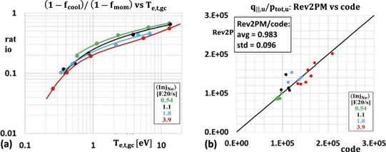
Figure 2. (a) The values of ![${\left[\frac{\left(1-{f}_{\text{cool}}\right)}{\left(1-{f}_{\text{mom}}\right)}\right]}^{\text{D}}$](https://content.cld.iop.org/journals/0029-5515/63/1/016017/revision4/nfac9917ieqn51.gif) for the database cases (points). The lines are best fits for
for the database cases (points). The lines are best fits for ![${\left[\frac{\left(1-{f}_{\text{cool}}\right)}{\left(1-{f}_{\text{mom}}\right)}\right]}^{\text{fit},\mathrm{D}}\left({T}_{\text{e},\mathrm{t},\mathrm{g}\mathrm{c}},\mathrm{I}\mathrm{n}{\mathrm{j}}_{\text{Ne}}\right)$](https://content.cld.iop.org/journals/0029-5515/63/1/016017/revision4/nfac9917ieqn52.gif) . The best fits for
. The best fits for  = 0.54; 1.1; 1.8 × 10²⁰ s−1 are, respectively, y = 0.1529 ln(x) + 0.2892 with R2 = 0.998; y = 0.1517 ln(x) + 0.2487 with R2 = 0.996; y = 0.1211 ln(x) + 0.2284 with R2 = 0.988; where y ≡
  and x ≡ Te,t,gc. For
  = 3.9 × 10²⁰ s−1, a log–log fit was used, R2 = 0.917, see appendix
 ![${\left[\frac{{q}_{\Vert,\mathrm{u}}}{{p}_{\text{tot},\mathrm{u}}}\right]}^{\text{Rev}2\mathrm{P}\mathrm{M},\mathrm{p}\mathrm{r}\mathrm{e}\mathrm{d}}$](https://content.cld.iop.org/journals/0029-5515/63/1/016017/revision4/nfac9917ieqn56.gif) vs
vs ![${\left[\frac{{q}_{\Vert,\mathrm{u}}}{{p}_{\text{tot},\mathrm{u}}}\right]}^{\text{code},\mathrm{T}}$](https://content.cld.iop.org/journals/0029-5515/63/1/016017/revision4/nfac9917ieqn57.gif) demonstrates that Rev2PM can fairly well predict the individual code values of
demonstrates that Rev2PM can fairly well predict the individual code values of  for the test cases from the individual code values of
  .
.
Download figure:
Standard image High-resolution imageOf course, the fit could just as well be done for ![$\left[\frac{\left(1-{f}_{\text{mom}}\right)}{\left(1-{f}_{\text{cool}}\right)}\right]$](https://content.cld.iop.org/journals/0029-5515/63/1/016017/revision4/nfac9917ieqn60.gif) rather than the reciprocal; however, use of the latter facilitates comparison of this lumped loss term with the individual volumetric power loss term, figure 9 of part A. As can be seen from equation (1b), the individual loss terms are in competition with regard to their effect on Te,t. In principle these terms might have cancelled or even reversed the direction of the Te,t—dependence on the lumped loss term; however, as can be seen from comparing figures 2(a) and 9 of part A, although it weakens it, the effect of momentum-loss does not overwhelm the effect of power-loss.
rather than the reciprocal; however, use of the latter facilitates comparison of this lumped loss term with the individual volumetric power loss term, figure 9 of part A. As can be seen from equation (1b), the individual loss terms are in competition with regard to their effect on Te,t. In principle these terms might have cancelled or even reversed the direction of the Te,t—dependence on the lumped loss term; however, as can be seen from comparing figures 2(a) and 9 of part A, although it weakens it, the effect of momentum-loss does not overwhelm the effect of power-loss.
The only other quantities that require fits are γsh and τt; as can be seen from figures 8(e) and (f) of part A, there is very little scatter in these quantities and so it is not worthwhile to make separate fits specifically for the database cases: for γsh (τt) the average of the ratio of (the code values for the database cases) to (the fit for all the cases) = 0.997 (0.994), with standard deviation = 0.010 (0.024), respectively; therefore, for these quantities the fits for all the cases were used,  and
and  . There is no significant InjNe—dependence for these quantities.
From equation (2) we then obtain:


The Rev2PM predicted values for the 21 test cases, ![${\left[\frac{{q}_{\Vert,\mathrm{u}}}{{p}_{\text{tot},\mathrm{u}}}\right]}^{\text{Rev}2\mathrm{P}\mathrm{M},\mathrm{p}\mathrm{r}\mathrm{e}\mathrm{d}}$](https://content.cld.iop.org/journals/0029-5515/63/1/016017/revision4/nfac9917ieqn63.gif) , are shown in figure 2(b). As can be seen,
, are shown in figure 2(b). As can be seen, ![${\left[\frac{{q}_{\Vert,\mathrm{u}}}{{p}_{\text{tot},\mathrm{u}}}\right]}^{\text{Rev}2\mathrm{P}\mathrm{M},\mathrm{p}\mathrm{r}\mathrm{e}\mathrm{d}}$](https://content.cld.iop.org/journals/0029-5515/63/1/016017/revision4/nfac9917ieqn64.gif) reproduces fairly well the code values for the test cases i.e.,
reproduces fairly well the code values for the test cases i.e., ![${\left[\frac{{q}_{\Vert,\mathrm{u}}}{{p}_{\text{totu}}}\right]}^{\text{code},\mathrm{T}}$](https://content.cld.iop.org/journals/0029-5515/63/1/016017/revision4/nfac9917ieqn65.gif) , without using any code data from the code test cases as input. From the viewpoint of understanding and scaling, this is the most important prediction of Rev2PM since, as noted earlier,
, without using any code data from the code test cases as input. From the viewpoint of understanding and scaling, this is the most important prediction of Rev2PM since, as noted earlier, ![$\left[\frac{{q}_{\Vert,\mathrm{u}}}{{p}_{\text{tot},\mathrm{u}}}\right]$](https://content.cld.iop.org/journals/0029-5515/63/1/016017/revision4/nfac9917ieqn66.gif) is the equivalent for Rev2PM to Te,t,gc for the 2PM.
is the equivalent for Rev2PM to Te,t,gc for the 2PM.
3.2. Testing the predictive capability of the Rev2PM for q||,u
We consider next the prediction for the upstream power flux density, q||,u, i.e.  , where we will use as input the target power flux density,
  . It should be noted that we want to avoid using as input the code values for the test cases i.e.
![${\left[{q}_{\Vert,\mathrm{t}}^{\text{TK}}\right]}^{\text{code},\mathrm{T}}$](https://content.cld.iop.org/journals/0029-5515/63/1/016017/revision4/nfac9917ieqn69.gif) , since we want the only required inputs to be
, since we want the only required inputs to be  . Thus we must first construct
 ![${\left[{q}_{\Vert,\mathrm{t}}^{\text{TK}}\right]}^{\text{fit},\mathrm{D}}\left({T}_{\text{e},\mathrm{t},\mathrm{g}\mathrm{c}},\mathrm{I}\mathrm{n}{\mathrm{j}}_{\text{Ne}}\right)$](https://content.cld.iop.org/journals/0029-5515/63/1/016017/revision4/nfac9917ieqn71.gif) and then check that it does adequately predict
and then check that it does adequately predict ![${\left[{q}_{\Vert,\mathrm{t}}^{\text{TK}}\right]}^{\text{code},\mathrm{T}}$](https://content.cld.iop.org/journals/0029-5515/63/1/016017/revision4/nfac9917ieqn72.gif) . Figure 3(a) shows
. Figure 3(a) shows ![${\left[{q}_{\Vert,\mathrm{t}}^{\text{TK}}\right]}^{\text{fit},\mathrm{D}}\left({T}_{\text{e},\mathrm{t},\mathrm{g}\mathrm{c}},\mathrm{I}\mathrm{n}{\mathrm{j}}_{\text{Ne}}\right)$](https://content.cld.iop.org/journals/0029-5515/63/1/016017/revision4/nfac9917ieqn73.gif) and figure 3(b) shows that
and figure 3(b) shows that ![${\left[{q}_{\Vert,\mathrm{t}}^{\text{TK}}\right]}^{\text{code},\mathrm{T}}$](https://content.cld.iop.org/journals/0029-5515/63/1/016017/revision4/nfac9917ieqn74.gif) is in fact fairly well predicted by
is in fact fairly well predicted by ![${\left[{q}_{\Vert,\mathrm{t}}^{\text{TK}}\right]}^{\text{fit},\mathrm{D}}\left({T}_{\text{e},\mathrm{t}\cdot \mathrm{g}\mathrm{c}}^{\text{code},\mathrm{T}},{\mathrm{I}\mathrm{n}\mathrm{j}}_{\text{Ne}}^{\text{code},\mathrm{T}}\right)$](https://content.cld.iop.org/journals/0029-5515/63/1/016017/revision4/nfac9917ieqn75.gif) .
.

Figure 3. (a) The values of ![${\left[{q}_{\Vert,\mathrm{t}}^{\text{TK}}\right]}^{\text{D}}$](https://content.cld.iop.org/journals/0029-5515/63/1/016017/revision4/nfac9917ieqn76.gif) , i.e. the code values of
, i.e. the code values of  for the database cases (points); the coefficients for the best log–log fits,
 ![${\left[{q}_{\Vert,\mathrm{t}}^{\text{TK}}\right]}^{\text{fit},\mathrm{D}}\left({T}_{\text{e},\mathrm{t},\mathrm{g}\mathrm{c}},\mathrm{I}\mathrm{n}{\mathrm{j}}_{\text{Ne}}\right)$](https://content.cld.iop.org/journals/0029-5515/63/1/016017/revision4/nfac9917ieqn78.gif) (lines), are given in appendix
(lines), are given in appendix ![${\left[{q}_{\Vert,\mathrm{t}}^{\text{TK}}\right]}^{\text{fit},\mathrm{D}}\left({T}_{\text{e},\mathrm{t},\mathrm{g}\mathrm{c}}^{\text{code},\mathrm{T}},{\mathrm{I}\mathrm{n}\mathrm{j}}_{\text{Ne}}^{\text{code},\mathrm{T}}\right)$](https://content.cld.iop.org/journals/0029-5515/63/1/016017/revision4/nfac9917ieqn79.gif) vs
vs ![${\left[{q}_{\Vert,\mathrm{t}}^{\text{TK}}\right]}^{\text{code},\mathrm{T}}$](https://content.cld.iop.org/journals/0029-5515/63/1/016017/revision4/nfac9917ieqn80.gif) demonstrates that Rev2PM can fairly well replicate the individual code values of
demonstrates that Rev2PM can fairly well replicate the individual code values of  for the test cases from the individual code values of
  .
.
Download figure:
Standard image High-resolution imageWe can now proceed to calculate  :
:


Equation (4) also uses the fit ![${\left[\left(1-{f}_{\text{cool}}\right)\right]}^{\text{fit},\mathrm{D}}\left({T}_{\text{e},\mathrm{t},\mathrm{g}\mathrm{c}},\mathrm{I}\mathrm{n}{\mathrm{j}}_{\text{Ne}}\right)$](https://content.cld.iop.org/journals/0029-5515/63/1/016017/revision4/nfac9917ieqn84.gif) , which is shown in figure 4.
, which is shown in figure 4.
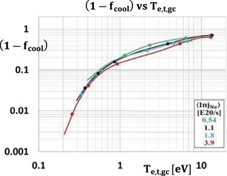
Figure 4. The values of ![${\left[\left(1-{f}_{\text{cool}}\right)\right]}^{\text{D}}$](https://content.cld.iop.org/journals/0029-5515/63/1/016017/revision4/nfac9917ieqn85.gif) , i.e. the code values of
, i.e. the code values of  for the database cases (points); the coefficients for the best log–log fits,
 ![${\left[\left(1-{f}_{\text{cool}}\right)\right]}^{\text{fit},\mathrm{D}}\left({T}_{\text{e},\mathrm{t},\mathrm{g}\mathrm{c}},\mathrm{I}\mathrm{n}{\mathrm{j}}_{\text{Ne}}\right)$](https://content.cld.iop.org/journals/0029-5515/63/1/016017/revision4/nfac9917ieqn87.gif) (lines), are given in appendix
(lines), are given in appendix
Download figure:
Standard image High-resolution imageFigure 5 shows that  predicts fairly well the code values of
  . The agreement is in fact rather better than for
 ![${\left[\frac{{q}_{\Vert,\mathrm{u}}}{{p}_{\text{tot},\mathrm{u}}}\right]}^{\text{Rev}2\mathrm{P}\mathrm{M},\mathrm{p}\mathrm{r}\mathrm{e}\mathrm{d}}$](https://content.cld.iop.org/journals/0029-5515/63/1/016017/revision4/nfac9917ieqn90.gif) , see figure 2(b).
, see figure 2(b).

Figure 5. The plot of  vs
vs ![${\left[{q}_{\Vert,\mathrm{u}}\right]}^{\text{code},\mathrm{T}}$](https://content.cld.iop.org/journals/0029-5515/63/1/016017/revision4/nfac9917ieqn92.gif) demonstrates that Rev2PM fairly well replicates the individual code values of q||,u for the test cases.
demonstrates that Rev2PM fairly well replicates the individual code values of q||,u for the test cases.
Download figure:
Standard image High-resolution imageFrom the practical viewpoint, the Rev2PM prediction for q||u is possibly more important than ![$\left[\frac{{q}_{\Vert,\mathrm{u}}}{{p}_{\text{tot},\mathrm{u}}}\right]$](https://content.cld.iop.org/journals/0029-5515/63/1/016017/revision4/nfac9917ieqn93.gif) . The most critical boundary values for the confined plasma are typically considered to be ne,u and PSOL. The latter is directly related to q||,u, although (experimentally) also involving the somewhat uncertain value of the SOL parallel power width.
. The most critical boundary values for the confined plasma are typically considered to be ne,u and PSOL. The latter is directly related to q||,u, although (experimentally) also involving the somewhat uncertain value of the SOL parallel power width.
3.3. Testing the predictive capability of the Rev2PM for ptot,u
We turn next to the Rev2PM prediction for the upstream total pressure, ptot,u, i.e.  , which is given by the mathematical identity:

Figure 6 shows that  predicts fairly well the code values of
  . The quality of the match is about the same as for
 ![$\left[\frac{{q}_{\Vert,\mathrm{u}}}{{p}_{\text{tot},\mathrm{u}}}\right]$](https://content.cld.iop.org/journals/0029-5515/63/1/016017/revision4/nfac9917ieqn97.gif) , since the match for q||u was much better than for
, since the match for q||u was much better than for ![$\left[\frac{{q}_{\Vert,\mathrm{u}}}{{p}_{\text{tot},\mathrm{u}}}\right]$](https://content.cld.iop.org/journals/0029-5515/63/1/016017/revision4/nfac9917ieqn98.gif) . Results, not shown here, are quite similar for
. Results, not shown here, are quite similar for ![${{p}_{\text{tot},\mathrm{u}}}^{\text{Rev}2\mathrm{P}\mathrm{M},\mathrm{p}\mathrm{r}\mathrm{e}\mathrm{d}}={\left[{p}_{\text{tot},\mathrm{t}}\right]}^{\text{fit},\mathrm{D}}\left({T}_{\text{e},\mathrm{t},\mathrm{g}\mathrm{c}}^{\text{code},\mathrm{T}},{\mathrm{I}\mathrm{n}\mathrm{j}}_{\text{Ne}}^{\text{code},\mathrm{T}}\right)/{\left[\left(1-{f}_{\text{mom}}\right)\right]}^{\text{fit},\mathrm{D}}\left({T}_{\text{e},\mathrm{t},\mathrm{g}\mathrm{c}}^{\text{code},\mathrm{T}},{\mathrm{I}\mathrm{n}\mathrm{j}}_{\text{Ne}}^{\text{code},\mathrm{T}}\right)$](https://content.cld.iop.org/journals/0029-5515/63/1/016017/revision4/nfac9917ieqn99.gif) .
.

Figure 6. The plot of  vs
vs ![${\left[{p}_{\text{tot},\mathrm{u}}\right]}^{\text{code},\mathrm{T}}$](https://content.cld.iop.org/journals/0029-5515/63/1/016017/revision4/nfac9917ieqn101.gif) demonstrates that Rev2PM can fairly well replicate the individual code values of ptot,u for the test cases.
demonstrates that Rev2PM can fairly well replicate the individual code values of ptot,u for the test cases.
Download figure:
Standard image High-resolution image3.4. Testing the predictive capability of the Rev2PM for Te,u
We turn next to the Rev2PM prediction for the upstream electron temperature, Te,u, i.e.  , which we will take here to be given by:

The basis for this simple estimate, which assumes the approximation that q|| is carried entirely by Spitzer parallel electron heat conduction, is discussed, e.g. in section 4.10 of [3]. For ft3, L||,div = 20.5 m. Here κe,||,0 = 2597 has been used without any Zeff correction [6]. Results are shown in figure 7(a). As can be seen,  predicts fairly well the code values of
  , although there is very little variation among the cases, which is to be expected because of (i) the 2/7th power involved, and (ii) the fact that
  varies little, figure 5, for these specific ITER cases all of which have PSOL = 100 MW.

Figure 7. (a) The plot of  vs
vs ![${\left[{T}_{\text{e},\mathrm{u}}\right]}^{\text{code},\mathrm{T}}$](https://content.cld.iop.org/journals/0029-5515/63/1/016017/revision4/nfac9917ieqn107.gif) demonstrates that Rev2PM can fairly well replicate the individual code values of Te,u. Also shown is the comparison for the ions, i.e. of
demonstrates that Rev2PM can fairly well replicate the individual code values of Te,u. Also shown is the comparison for the ions, i.e. of  and
and ![${\left[{T}_{\text{i},\mathrm{u}}\right]}^{\text{code},\mathrm{T}}$](https://content.cld.iop.org/journals/0029-5515/63/1/016017/revision4/nfac9917ieqn109.gif) , see the text for details, also indicating that Rev2PM can fairly well replicate the individual code values of Ti,u for the test cases. (b) The plot of
, see the text for details, also indicating that Rev2PM can fairly well replicate the individual code values of Ti,u for the test cases. (b) The plot of  as a function of individual values of InjNe, for the database cases only, indicates a strong correlation: the red line is the best quadratic fit, y = −4.03E − 38x2 + 1.99E − 16x + 8.55E + 04, where
  and x ≡ InjNe; R2 = 0.865.
Download figure:
Standard image High-resolution imageFor the Rev2PM prediction for the upstream ion temperature, Ti,u, i.e.  , we will use the strong correlation that has been found in the present code results between
  and InjNe, see figure 7(b) which is for the database cases only. This provides the functional relation
 ![$\left[{\tau }_{\text{u}}^{\text{code},\mathrm{D}}\right]\left(\mathrm{I}\mathrm{n}{\mathrm{j}}_{\text{Ne}}\right)$](https://content.cld.iop.org/journals/0029-5515/63/1/016017/revision4/nfac9917ieqn114.gif) . The values of
. The values of  are then given by:

Results are also shown in figure 7(a).
3.5. Testing the predictive capability of the Rev2PM for ne,u
Finally we obtain the Rev2PM prediction for the upstream electron density, ne,u, i.e.  , which is given by:


where the upstream Mach number  is assumed to be small enough that
  . Figure 8(a) shows that
  fairly well predicts the code values of
  , and as for the other upstream quantities, this is done without using any code data from the code test cases as input. The quality of the match is about the same as for
 ![$\left[\frac{{q}_{\Vert,\mathrm{u}}}{{p}_{\text{tot},\mathrm{u}}}\right]$](https://content.cld.iop.org/journals/0029-5515/63/1/016017/revision4/nfac9917ieqn121.gif) and ptot,u.
and ptot,u.

Figure 8. (a) The plot of  vs
vs ![${\left[{n}_{\text{e},\mathrm{u}}\right]}^{\text{code},\mathrm{T}}$](https://content.cld.iop.org/journals/0029-5515/63/1/016017/revision4/nfac9917ieqn123.gif) demonstrates that Rev2PM can fairly well replicate the individual code values of ne,u for the test cases from the individual code values of
demonstrates that Rev2PM can fairly well replicate the individual code values of ne,u for the test cases from the individual code values of  . (b) The same as (a) but using the 2PM expressions that explicitly take into account the power loss to the electrons due to recycle of the deuterium, rather than directly including it with the other losses.
Download figure:
Standard image High-resolution imageEquations (1) and (2) are the 2PM expressions that are appropriate when the energy loss to the electrons due to ionization of the recycling neutral deuterium is not explicitly taken into account, but is instead directly included with the other electron power losses. The expressions are somewhat different when the recycle power loss is included explicitly, see e.g. section 5.5 of [3], equation (4) of [5], etc. The above Rev2PM analysis requires some small modifications in order to take recycle power loss explicitly into account, resulting in small changes in the figures starting with figure 1. Details will be reported elsewhere. Here we only report the result for ne,u, figure 8(b). As can be seen, the effect of taking recycle energy loss explicitly into account is small; however, it does provide a somewhat better match to the code.
As an aside: it is evident from figure 8 that there is a strong correlation between ne,u and InjNe. The related correlation between ne,u and ⟨cz⟩sep was pointed out in [7], see figure 15 there and accompanying text, ( (where the sum is over the charge states of species Z) is the impurity concentration averaged along the separatrix upstream of the X-point) where it is noted that this may have important implications for ITER baseline operation:
'Returning to the question of maximum tolerable ne,sep, the highest values in figure 15(a) ... are found at the lowest cNe and peak at ne,sep ∼ 6 × 10¹⁹ m−3* 4 . This is 0.5 nGW for the 15 MA ITER baseline burning plasma.... The analysis in [93 of [1]], finds the observed H-mode operational boundary to be roughly limited by ne,sep/nGW < 0.4–0.5 in JET and ASDEX Upgrade.... If the same limit also applies to ITER, then the lowest seeding values in the SOLPS-4.3 database would be marginal, .... Since the lower cNe are those at which QDT is maximized [3 of [1]], a compromise will need to be sought for the appropriate seeding level, assuming Ne as extrinsic radiator and depending on the real λq which is found on ITER. What is clear is that more simulations are required, particularly at reduced transport in the W/Be environment with impurity seeding (Ne and N)'.
4. Summary, discussion and conclusion
In summary, it is sufficient to specify the value of the variable pair  ,
,  alone, for the Rev2PM to be able to predict the values of all upstream (divertor-entrance) quantities of practical interest. The specified values of
  ,
,  may be any values within the ranges (for the database cases) of the variables used to make the numerical fits needed to quantitatively characterize the Rev2PM. Further, since all the target quantities of practical interest are strongly correlated with the same variable pair,
  ,
,  , database fits, e.g. for
  , figure 3(a), can also be used to predict the values for all the target quantities of practical interest as well. Therefore it is sufficient to specify the value of
  ,
,  to be able to reproduce the values of all the major target and divertor-entrance quantities calculated by S-I for ITER baseline conditions.
As noted earlier, only a limited test of predictive capability could be carried out within the context of this report, based on dividing the set of 41 cases into two subsets. All the cases used in this report are for ITER baseline burning plasma conditions, QDT = 10, q95 = 3, PSOL = 100 MW, metallic walls, and Ne seeding; they do not include different values of PSOL or pumping speed, nor other impurity species, nor classical currents or drifts, nor different ad hoc radial transport coefficients, etc. Extensions of the present study will therefore be required to be able to draw more definitive conclusions.
As discussed in section 1, it would be valuable to have, if possible, a comprehensive Rev2PM reduced model for the ITER divertor, i.e. a single model that would cover a range of PSOL values and of other critical inputs such as the assumed values of the radial transport coefficients, χ⊥, D⊥, or the power width, λq,||, etc, that is a reduced model whose sole inputs would be  . It remains to be seen if this will be possible. If it is not, then an alternative approach to the Rev2PM is to use a reduced model based purely on numerical fits for the upstream quantities, similar to the ones in sections 3–5 of part A for the target quantities. Here we will call this the fully fit-based reduced model, to distinguish it from the Rev2pm reduced model. Of course, the latter also uses numerical fits, but the former is purely fit-based and does not use Rev2PM.
Consider, for example, the key quantity ne,u. The lines in figure 9(a) are ![${\left[{n}_{\text{e},\mathrm{u}}\right]}^{\text{fit},\mathrm{D}}\left({T}_{\text{e},\mathrm{t},\mathrm{g}\mathrm{c}},\mathrm{I}\mathrm{n}{\mathrm{j}}_{\text{Ne}}\right)$](https://content.cld.iop.org/journals/0029-5515/63/1/016017/revision4/nfac9917ieqn138.gif) and were constructed in the same way as the fits in figures 2(a), 3(a) and 4, i.e. using the database cases only. Figure 9(b) shows that
and were constructed in the same way as the fits in figures 2(a), 3(a) and 4, i.e. using the database cases only. Figure 9(b) shows that ![${\left[{n}_{\text{e},\mathrm{u}}\right]}^{\text{code},\mathrm{T}}$](https://content.cld.iop.org/journals/0029-5515/63/1/016017/revision4/nfac9917ieqn139.gif) is about as well predicted by
is about as well predicted by ![${\left[{n}_{\text{e},\mathrm{u}}\right]}^{\text{fit},\mathrm{D}}\left({T}_{\text{e},\mathrm{t},\mathrm{g}\mathrm{c}}^{\text{code},\mathrm{T}},{\mathrm{I}\mathrm{n}\mathrm{j}}_{\text{Ne}}^{\text{code},\mathrm{T}}\right)$](https://content.cld.iop.org/journals/0029-5515/63/1/016017/revision4/nfac9917ieqn140.gif) as by the Rev2PM reduced model, compare figure 8. It seems less likely, however, that it will be possible to develop a comprehensive fully fit-based reduced model than a comprehensive Rev2PM reduced model: for the former it would seem necessary to calculate separate
as by the Rev2PM reduced model, compare figure 8. It seems less likely, however, that it will be possible to develop a comprehensive fully fit-based reduced model than a comprehensive Rev2PM reduced model: for the former it would seem necessary to calculate separate ![${\left[{n}_{\text{e},\mathrm{u}}\right]}^{\text{fit},\mathrm{D}}\left({T}_{\text{e},\mathrm{t}},\mathrm{I}\mathrm{n}{\mathrm{j}}_{\text{Ne}}\right)$](https://content.cld.iop.org/journals/0029-5515/63/1/016017/revision4/nfac9917ieqn141.gif) for each value of PSOL, although this remains to be seen.
for each value of PSOL, although this remains to be seen.

Figure 9. (a) The values of ![${\left[{n}_{\text{e},\mathrm{u}}\right]}^{\text{D}}$](https://content.cld.iop.org/journals/0029-5515/63/1/016017/revision4/nfac9917ieqn142.gif) , i.e. the code values of ne,u for the database cases (points); the coefficients for the best log–log fits,
, i.e. the code values of ne,u for the database cases (points); the coefficients for the best log–log fits, ![${\left[{n}_{\text{e},\mathrm{u}}\right]}^{\text{fit},\mathrm{D}}\left({T}_{\text{e},\mathrm{t},\mathrm{g}\mathrm{c}},\mathrm{I}\mathrm{n}{\mathrm{j}}_{\text{Ne}}\right)$](https://content.cld.iop.org/journals/0029-5515/63/1/016017/revision4/nfac9917ieqn143.gif) (lines), are given in appendix
(lines), are given in appendix ![${\left[{n}_{\text{e},\mathrm{u}}\right]}^{\text{fit},\mathrm{D}}\left({T}_{\text{e},\mathrm{t},\mathrm{g}\mathrm{c}}^{\text{code},\mathrm{T}},{\mathrm{I}\mathrm{n}\mathrm{j}}_{\text{Ne}}^{\text{code},\mathrm{T}}\right)$](https://content.cld.iop.org/journals/0029-5515/63/1/016017/revision4/nfac9917ieqn144.gif) vs
vs ![${\left[{n}_{\text{e},\mathrm{u}}\right]}^{\text{code},\mathrm{T}}$](https://content.cld.iop.org/journals/0029-5515/63/1/016017/revision4/nfac9917ieqn145.gif) shows that the fully fit-based reduced model replicates the individual code values of ne,u for the test cases from the individual code values of
shows that the fully fit-based reduced model replicates the individual code values of ne,u for the test cases from the individual code values of  about as well as the Rev2PM reduced model, see figure 8.
Download figure:
Standard image High-resolution imageWhat has been achieved so far then is that (a) two limited-scope reduced models for the ITER divertor have been developed, and (b) a general procedure has been identified for constructing a Rev2PM reduced model as well a fully fit-based reduced model for a tokamak divertor based on a set of code results for the tokamak. It remains to be seen if comprehensive reduced models can be found, even just for ITER.
Finally, it should be noted that, so long as these reduced models are based on phenomenological, numerical correlations, e.g. for  , then, strictly, they can only be used to make projections to lower values of Te,t,gc than were used to make the numerical fits used in the reduced models, and not true predictions: the latter would require a physics-based model for the functional relationships, e.g.
 ![$\left[1-{f}_{\text{cool}}\right]\left({T}_{\text{e},\mathrm{t},\mathrm{g}\mathrm{c}},\mathrm{I}\mathrm{n}{\mathrm{j}}_{\text{Ne}}\right)$](https://content.cld.iop.org/journals/0029-5515/63/1/016017/revision4/nfac9917ieqn148.gif) , valid for the required range of
, valid for the required range of  values.
Here in part B of the study, reversed-direction two point modeling, Rev2PM, was identified as a limited-scope (because of a single value of PSOL, primarily) reduced model that is able to directly and readily take advantage of using  for its reduced model control parameters, i.e. its input, since these are either downstream or global quantities. In standard, i.e. forward-direction 2PM, the independent variables, i.e. the inputs, are the upstream quantities, q||,u and ptot,u, and the dependent variables, i.e. the outputs, are target quantities such as Te,t,gc. In reversed-direction 2PM, Rev2PM, the independent variables, i.e. the inputs, are target quantities, e.g. Te,t,gc, and/or specified global quantities, e.g. InjNe, while the dependent variables, i.e. the outputs, are upstream quantities, e.g. q||,u and ptot,u.
In the present study, three steps have thus been taken toward the development of a (comprehensive) reduced model for the ITER divertor based on reversed-direction two point modeling, Rev2PM:
- (a)In part A, a pair of promising reduced model control parameters have been identified, [Te,t,gc, InjNe].
- (b)In part B, the Rev2PM has been identified as a (limited-scope, at least) reduced model that can logically and easily use [Te,t,gc, InjNe] as inputs, since these are downstream or global control parameters.
- (c)In part B, a first, limited test of the predictive capability of the reduced model was successfully carried out: the present set of 41 ITER cases was divided into two subsets: (a) a subset of 20 database cases, and (b) a subset of 21 test cases. The database cases (only) were used to make the fits needed to apply the Rev2PM to the test cases, and demonstrated reasonable reliability for the Rev2PM predictions.
At this point it is not known if the Rev2PM can provide the basis for a comprehensive reduced model for the ITER divertor since the database of cases used in the present study is too narrow. Extensions of the present study will therefore be required to be able to draw more definitive conclusions.
As was shown in figure 8, values of ne,u calculated using the fully fit-based reduced model, FFBRM, reproduce the individual code values about as well as the Rev2PM reduced model, Rev2PMRM. This is as to be expected since, strictly 'Rev2PM' should be designated as 'Rev2PMF', where the 'F' stands for formatting, see section 11 'two point model formatting of EDGE2D, SOLPS, SONIC, UEDGE, etc code output' of [2]: all the 2PM and Rev2PM expressions used here are identically true if the individual values of Te,t,gc, (1 − fmom), etc for each case are used in the expressions, e.g. equations (1b) and (2). The first step toward a true model involves using numerical fits to e.g. (1 − fmom)[Te,t,gc], etc, as has been done in the present work. As just noted, the next step will be to develop more comprehensive reduced models based on code cases for a range of values of PSOL, etc, if that is possible. However, a model with full predictive capability will require that quantities like (1 − fmom)[Te,t,gc] be obtained using information from other sources than codes, for example, from first-principle physics models or from experimental measurements. A potentially useful step short of full predictive capability will be possible if it is found that a variety of codes give similar results for key quantities like (1 − fmom)[Te,t,gc].
This still leaves the question that if, for example, the values of ne,u calculated using the FFBRM reproduce the individual code values about as well as the Rev2PMRM does, then why bother with the latter? As noted earlier, it seems less likely that it will be possible to develop a comprehensive FFBRM than a comprehensive Rev2PMRM: for the former it would seem likely that it will be necessary to calculate ![${\left[{n}_{\text{e},\mathrm{u}}\right]}^{\text{fit},\mathrm{D}}\left({T}_{\text{e},\mathrm{t},\mathrm{g}\mathrm{c}},\mathrm{I}\mathrm{n}{\mathrm{j}}_{\text{Ne}}\right)$](https://content.cld.iop.org/journals/0029-5515/63/1/016017/revision4/nfac9917ieqn151.gif) , etc, for each value of PSOL, etc. It also seems likely that physical understanding will be better aided by Rev2PMRM than by FFBRM, but this remains to be seen.
, etc, for each value of PSOL, etc. It also seems likely that physical understanding will be better aided by Rev2PMRM than by FFBRM, but this remains to be seen.
High quality experimental results are now emerging from present day tokamak studies for a number of the quantities reported in this study, and can be compared with the above code results for ITER to assess their general plausibility. It will also be informative to apply the general procedure developed in this study to construct a reduced model of the divertor based on a set of code results for a presently operating tokamak, thus making it possible to test predictions of the reduced model with experimental measurements in the near term.
The methodology presented here is a step on the path toward the development of reduced models which could be transferred, eventually, to real tokamak operational control, or the implementation of simple descriptions of the complex processes at work in the divertor which could be used in pulse design simulators. Such simulators need to be fast so that they can be used to turn around a pulse design in a matter of minutes for use in planning discharges on ITER.
The data set used in this report is restricted to baseline ITER conditions, i.e. PSOL = 100 MW, etc, an important limitation of the scope and potential application of this study that has to be kept in mind. With regard to absolute values, and possibly even to the trends, the findings here may not apply generally for ITER, e.g. to other values of PSOL, let alone to other tokamaks.
Acknowledgments
This manuscript has been authored by UT-Battelle, LLC under Contract No. DE-AC05-00OR22725 with the US Department of Energy. The United States Government retains and the publisher, by accepting the article for publication, acknowledges that the United States Government retains a non-exclusive, paid-up, irrevocable, world-wide license to publish or reproduce the published form of this manuscript, or allow others to do so, for United States Government purposes. The Department of Energy will provide public access to these results of federally sponsored research in accordance with the DOE Public Access Plan (http://energy.gov/downloads/doe-public-access-plan). The views and opinions expressed herein do not necessarily reflect those of the ITER Organization.
Appendix A: Definitions of the quantities used in this report.
For simplicity, the subscript 'gc' is usually dropped in appendix A, and it is to be understood that Te,t ≡ Te,t,gc.
The following is an extension of [2]. There are four components of q||, the parallel power flux density carried by the plasma, i.e. by the charged particles|: (i) thermal energy, kT, (T) (ii) kinetic energy, mnv2, (K) (iii) potential energy of ionization and molecular dissociation,  , (P), and (iv) −jV electrostatic potential energy, (J). A derivation of the −jV term is given in appendix B; however, it should be noted that for the cases used here, plasma currents, as well as drifts, were turned off, i.e. j = 0. As discussed e.g. in [2], the target sheath causes plasma cooling by removing the plasma's thermal and kinetic energy. The sheath heat transmission coefficient for plasma cooling,
  , is therefore defined by:

It can be shown that, approximately  [3], and thus with several further approximations the result is:

where the further approximations are to assume: (i)  , the isothermal plasma sound speed at the target, (ii) Ti,t = Te,t, (iii) no plasma impurities, and (iv) Mach 1 flow at the target. It should be noted, however, that in this paper the full expression, equation (A1), is used to evaluate
  using the S-I output values of
  , Te,t,gc and Γ||,e,t.
Here, with the aim of being more explicit, compact and hopefully clearer, we will define:

As discussed in section 11 of [2] on two point model formatting, the plasma cooling factor,  , is defined by:

see equation (64) of [2]. The volumetric momentum loss factor,  , is defined similarly, equation (65) of [2]. Here, to be more explicit and clear we will use:


As discussed, e.g. in [2], the power flux density deposited on the target by the plasma includes three energy components (T, K and P), minus the power reflected as neutrals by ions incident on the target, thus:

where θ⊥ is the incidence angle between B and the target surface and:

where the (recombination) potential energy  15 eV. Figure A1 compares
  and
and  where, as can be seen, simply assuming a constant
  = 14.2 eV gives a quite close match.

Figure A1.
 and
and  , Tet < 15 eV. As can be seen, simply assuming a constant
  = 14.2 eV gives a close match.
Download figure:
Standard image High-resolution imageNote that ions that are reflected as atoms do not deposit  , and in principle this should be allowed for. For refractory metals, the fraction of ions reflected as neutrals, as well as the fraction of incident energy carried by the reflected atom can be quite high. Figure A2 shows
  and
and  vs Te,t.

Figure A2.
 and
and  for ft3, Tet < 15 eV.
Download figure:
Standard image High-resolution imageAs can be seen for these cases,  is small relative to
  but not negligible. Since the primary purpose of the present report is to identify control parameters,
  is used rather than
  , etc; however, when comparisons with experiment are involved, the difference should be used.
Here we will use: 
In [2] the power loss factor
 is defined by:


In section 2 it was noted that there is little difference between  and
and , and we can simply use q||,u. Since
  , then
  , and so
 , which is illustrated in figure A3. From the above it is readily shown that:


Figure A3.

 and
and 
 vs Te,t. The open red circles are for
  which for
  = 14.2 eV, constant, is expected to equal
  approximately, see equation (A12).
Download figure:
Standard image High-resolution imageThe total power flux density deposited on the target by the plasma plus neutrals & photons is:

where θ⊥ is the incidence angle between B and the target surface. For the ITER outer target, the toroidally symmetric value is θ⊥ = 2.7° in the strike point vicinity [7]; with target toroidal tilting and divertor tungsten monoblock surface beveling (to avoid exposed leading edges), the angle between B and the toroidally asymmetric outer target surface is increased to θ⊥ = 4.2°.
The term qdep,neut,t allows for the power carried by the reflected neutrals, and thus may even be negative in principle at certain spatial locations, although of course the power flux density  integrated over the entire plasma facing surface must be equal to the power entering the simulation through the core or via 'external' volumetric sources.
The physical validity of the −jV component of q||,t has sometimes been questioned; it is discussed in appendix B. When included then the variable is  , where 'V' is for electrostatic potential energy, to be distinguished from recombination potential energy which is indicated by 'P'. As noted, for the present cases j = 0.
Appendix B.: Derivation of the sheath heat transmission coefficient including the −jV electrostatic potential energy term
The following extends the analysis in section 25.5 of [3] 'Expressions for the Floating Potential, Particle and Heat Flux Densities Through the Sheath', to now include a derivation of the −jV term. In [3] it was simply stated without proof on page 652 that 'The power removed from the plasma as a function of V is qse(V) = qsurface(V) − jTOT(V)|V|. It is important to distinguish between the power to biased and floating surfaces, i.e. equation (25.54) versus equation (25.46), [25.30, 25.31]'. In the following the −jV term is derived.
The current density j(≡jTOT) from the plasma to the target is given by:

where Γi(e) is the ion (electron) particle flux density.
At the sheath edge, se, the thermal energy removed from the plasma electrons (thereby cooling them) by the target sheath is:

where V is the electrostatic potential of the target; the reference potential is taken here to be at the se, i.e. Vse = 0. For an electrically floating target V < 0. Targets are almost never biased such that V > 0, owing to the extremely large (damaging) current of electrons that would result. Thus, usually −eV is positive, and −eV  3eTe for hydrogenic plasmas and floating targets.
At the sheath edge, se, the thermal energy removed from the plasma ions (thus cooling them) by the target sheath is:

where the value of the numerical coefficient depends on assumptions made about the amount of thermal energy convected by the ions in the pre-sheath, i.e. the plasma upstream of the sheath entrance, see section 25.1 of [3]. In SOLPS the factor is 3.5, and we will use that value in the following for concreteness .
Table A1. Table of variable names. Concentrations are defined as  , where i and j are radial and poloidal cell indices of the numerical simulation grid.
  ,where V is the cell volume.
  , where k indicates charge state. Simply connected lower single null, LSN, grids are assumed, where the poloidal cell index of the outer target guard cell is nx, and the cell just 'in front' of the target has the poloidal index nx − 1. Radial index isep + 1 is the first set of cells outside the separatrix. Note that
  is used as the upstream index, essentially where the peak in q|| occurs.
| Description | Symbol | S-I var. name(s) | Source | Indices |
|---|---|---|---|---|
| Density of ion | na | NA | b2fstate | i, j |
| Volume of cell | V | VOL | b2fgmtry | i, j |
| Puff strength D2 | InjD | USERFLUXPARM | b2.neutrals.parameters | D2 gas puff stratum |
| Puff strength neon | InjNe | USERFLUXPARM | b2.neutrals.parameters | Neon gas puff stratum |
| Flux tube neon concentration |

| — | Post-processed |

|
| Flux tube neon concentration |

| — | Post-processed |
 , , |
| i ∈ {jsep, jsep + 1} {Thi | ||||
| Deuterium atom | nD,t | DAB2 | fort.44 | j = nx − 1 |
| Deuterium molecular | nD2,t | DMB2 | fort.44 | j = nx − 1 |
| Guard cell electron density | ne,t,gc | NE | b2fstate | j = nx |
| Average neutral pressure |

| DAB2 X TAB2 + DMB2 X TMB2 | Post-processed from | See figure 1 |
| B2PLOT USER routine, input | ||||
| ig = ny + 1 | ||||
| Total plasma pressure at target | ptot,t | — | Postprocessed from b2fstate | j = nx − 1 |
| Total plasma pressure upstream | ptot,u | — | Postprocessed from b2fstate |
j = 
|
| Parallel heat flux density at the target |

| (FHTX − FHJX)/PBSX | Postprocessed from B2PLOT a | j = nx |
| Parallel heat flux density upstream |

| (FHTX − FHJX)/PBSX | Postprocessed from B2PLOT a |
j = 
|
| Potential energy flux density at target |

| FHPX/PBSX | Postprocessed from B2PLOT a | j = nx |
| Potential energy flux density upstream |

| FHPX/PBSX | Postprocessed from B2PLOT a |
j = 
|
| Electrostatic energy flux at target |

| FHJX/PBSX | Postprocessed from B2PLOT a | j = nx |
| Electron temperature at target | Te,t,lc | TE | b2fstate | j = nx − 1 |
| Electron temperature in guard cell | Te,t,gc ≡ Te,t | TE | b2fstate | j = nx |
| Ion temperature at target | Ti,t,lc | TI | b2fstate | j = nx − 1 |
| Ion temperature in guard cell | Ti,t,gc | TI | b2fstate | j = nx |
| Power to target from neutral particles | qneut,t | WNEUT | j = nx | |
| Power to target from radiation | qrad,t | WRAD | Post-processed from B2PLOT a 100 WLLD | j = nx |
| Total neutral flux to target | ΓD,sum,t | D_FLUX_ATM + 2x a 2_FLUX_MOL | Post-processed from B2PLOT a 100 WLLD | j = nx |
| Parallel electron particle | Γ||,e,t | SUM(FNA/PBSX) | B2PLOT a , note: neglecting poloidal | j = nx |
aB2PLOT is a postprocessing program packaged as part of the S-I code. In the table above the arguments to the routine, variable names, and indices are given where appropriate.
As the electrons pass through the sheath they each lose an amount of kinetic energy equal to −eV in the retarding electric field of the sheath by the point they reach the solid surface, where they are deposited. Thus the thermal energy deposited on the surface by the electrons is:

As the ions pass through the sheath they each gain an amount of kinetic energy equal to −eV in the attracting electric field of the sheath by the point they reach the solid surface, where they also deposit. Thus the thermal plus kinetic energy deposited on the surface by the ions is:

The totals are therefore:


which is the result stated without proof on page 652 of [3].
Such a mathematical exercise may leave one still feeling unclear about what is happening physically. Consider a thought experiment where V becomes more negative than Vfloating, i.e. |V| becomes larger and so Γe decreases. Thus  increases, becoming positive. Thus from equation (B8) qe+i,surf > qe+i,se,cool and also qi,surf − qi,se,cool = −ΓieV, which is positive, i.e. the impact energy of the ions on the target is increased. We may wonder how it is possible for more power to be deposited on the target than entered the sheath. The explanation is that we have not as yet considered the
electrostatic potential energy of the ions and electrons at the two different locations. At the se each ion has (positive) electrostatic potential energy ɛi,pot = e|V| relative to the target, while each electron has (negative) electrostatic potential energy ɛe,pot = −e|V|. For V = Vfloating, Γi = Γe and thus there is no net electrostatic potential energy deposited on the target when the e–i pair deposit there (there is, of course, the e–i recombination potential energy, but that is included separately, as discussed in appendix A). However, when V is more negative than Vfloating, then qi,pot,surf = Γie|V| (W m−2), qe,pot,surf = −Γee|V| (W m−2), and
increases, becoming positive. Thus from equation (B8) qe+i,surf > qe+i,se,cool and also qi,surf − qi,se,cool = −ΓieV, which is positive, i.e. the impact energy of the ions on the target is increased. We may wonder how it is possible for more power to be deposited on the target than entered the sheath. The explanation is that we have not as yet considered the
electrostatic potential energy of the ions and electrons at the two different locations. At the se each ion has (positive) electrostatic potential energy ɛi,pot = e|V| relative to the target, while each electron has (negative) electrostatic potential energy ɛe,pot = −e|V|. For V = Vfloating, Γi = Γe and thus there is no net electrostatic potential energy deposited on the target when the e–i pair deposit there (there is, of course, the e–i recombination potential energy, but that is included separately, as discussed in appendix A). However, when V is more negative than Vfloating, then qi,pot,surf = Γie|V| (W m−2), qe,pot,surf = −Γee|V| (W m−2), and  (W m−2), which is positive since j > 0. This then explains where the apparently missing energy/power came from. An equivalent argument applies to the situation where V becomes less negative than Vfloating.
Appendix C.: The fitting procedure used
The fitting procedure used .excel polynomial fits. It was found convenient to first generate the fits using logarithmic values of the quantities, and then convert back to the values themselves. The numerical values of the log–log fit parameters are given in table C1.
Table C1. Polynomial fit coefficients for the log–log fits. y = ax4 + bx3 + cx2 + dx + e, where y = log(dependent variable) and x = log(independent variable).
| Figure | dependent variable | independent variable | a | b | c | d | e | R2 |
| 2a.4 a | (1 − fc)/(1 − fm) | Te,t,gc | −0.144 461 667 | 0.458 138 567 | −0.428 428 825 | 0.502 895 328 | −0.693 627 469 | 0.917 |
| 3a.1 a |

| Te,t,gc | 0.035 465 3727 | 0.141 084 131 | −0.651 254 906 | 1.009 724 27 | 7.694 892 95 | 0.999 |
| 3a.2 a |

| Te,t,gc | −0.641 012 006 | 1.296 714 93 | −0.933 316 251 | 0.845 008 876 | 7.674 263 93 | 0.999 |
| 3a.3 a |

| Te,t,gc | −1.247 390 13 | 2.026 465 77 | −1.071 506 99 | 0.690 673 584 | 7.713 269 44 | 0.999 |
| 3a.4 a |

| Te,t,gc | −1.161 351 36 | 1.957 950 57 | −0.787 572 771 | 0.632 895 878 | 7.583 794 18 | 0.999 |
| 4.1 | 1 − 
| Te,t,gc | 0.077 998 1122 | 0.096 756 0884 | −0.724 103 668 | 1.071 330 96 | −0.696 036 483 | 0.999 |
| 4.2 | 1 − 
| Te,t,gc | −0.536 138 518 | 1.176 515 19 | −1.019 099 07 | 0.937 207 54 | −0.728 959 293 | 0.999 |
| 4.3 | 1 − 
| Te,t,gc | −1.431 211 31 | 2.140 399 82 | −1.063 060 56 | 0.726 311 26 | −0.708 501 836 | 0.999 |
| 4.4 | 1 − 
| Te,t,gc | −1.020 846 45 | 1.834 714 23 | −0.921 557 828 | 0.726 005 873 | −0.825 420 658 | 0.999 |
| 9a.1 a | ne,Xpt | Te,t,gc | −0.227 456 696 | 0.351 570 479 | −0.268 267 958 | 0.060 971 8348 | 19.922 4712 | 0.999 |
| 9a.2 a | ne,Xpt | Te,t,gc | 0 | −0.041 252 9932 | −0.052 880 6776 | 0.079 120 0878 | 19.801 269 | 0.839 |
| 9a.3 a | ne,Xpt | Te,t,gc | 0 | 0.001 612 23456 | 0.005 588 895 517 | −0.029 945 7665 | 19.749 3639 | 0.209 |
| 9a.4 a | ne,Xpt | Te,t,gc | 0 | 0.240 516 625 | −0.332 525 131 | 0.007 918 862 69 | 19.719 0914 | 0.916 |
aThe numbers 1, 2, 3, 4 after the period indicate ⟨InjNe⟩ = 0.54, 1.1, 1.8, 3.9 (e20 atoms s−1) respectively.
Footnotes
- ∗
This manuscript has been partially authored by UT-Battelle, LLC, under Contract DE-AC05-00OR22725 with the US Department of Energy. This material is based upon work supported the Scientific Discovery through Advanced Computing (SciDAC) project on Plasma–Surface Interactions.
- 4
It should be noted that ne,sep in [7] is the density at the OMP on ft1, whereas ne,u here is the density at the Xpoint on ft3. OMP densities are significantly lower than Xpoint ones: for ft3,
= 3.98 × 10¹⁹ m−3, = 5.94 × 10¹⁹ m−3.

