


Abstract
Alfvénic activity has been observed in the TJ-II stellarator which resembles the frequency sweeping demonstrated by Alfvén cascade modes in tokamaks. A numerical validation study was conducted using a reduced magnetohydrodynamic (MHD) model to show that such modes could only have been observed in discharges where the rotational transform profile was non-monotonic. During experiments, coil current was varied which resulted in shifting of the minimum value of the rotational transform profile. To mimic this effect, we study the Alfvénic activity predicted by the reduced MHD model for a set of input rotational transform profiles with varying minima. A mode is found whose toroidal and poloidal mode numbers match those predicted in experiments which sweeps downward/upward in frequency as the minimum value of the rotational transform profile is increased/decreased. The results serve as a demonstration of the validity and utility of MHD spectroscopy.
Export citation and abstract BibTeX RIS

Original content from this work may be used under the terms of the Creative Commons Attribution 4.0 license. Any further distribution of this work must maintain attribution to the author(s) and the title of the work, journal citation and DOI.
1. Introduction
Alfvén eigenmodes present both challenges and opportunities to the magnetic confinement fusion community. Alfvén waves are a benign feature of all magnetized plasma systems, but they can be driven unstable in toroidal fusion devices by resonant charged fast particles, both fusion-born alpha particles and those introduced by external heating systems. Such interactions can have deleterious effects on fusion performance by driving alpha particles out of the plasma core and on device integrity by potentially damaging first wall components [1].
One class of Alfvén eigenmodes known as reversed shear Alfvén eigenmodes (RSAEs) [2–6] can, however, serve a diagnostic purpose through a technique called magnetohydrodynamic (MHD) spectroscopy [7]. RSAEs occur in toroidal devices when there is a local extremum in the safety factor (tokamaks) [8] or rotational transform (stellarators) profile [9]. Note that the rotational transform profile is the inverse of the safety factor and may also be referred to as an iota profile. In the following text, the terms rotational transform profile and iota profile are used interchangeably. The frequency of these modes sweeps upward or downward as the minimum value of the safety factor or rotational transform profile changes in time. Due to the sweeping behavior they exhibit, RSAEs are also referred to as Alfvén cascades.
MHD spectroscopy broadly refers to the indirect determination of bulk plasma parameters via direct measurements of MHD waves [2]; the specific MHD spectroscopy technique relevant to this work uses direct measurements of the frequency evolution of an Alfvén cascade to infer the evolution of the value of the rotational transform profile's minimum.
The first observation of Alfvén cascades was reported by the JT-60U team in 1998 [10]. Since then, they have been observed in tokamaks such as JET [11], DIII-D [12], ASDEX-U, MAST [13], and NSTX [14]. They have also been seen in the helical device LHD [9] and were suspected to be seen on TJ-II in [15]. The purpose of this work is to confirm using numerical modeling that the conditions in TJ-II can account for the production of modes of this type.
The paper is divided into the following sections: in section 2, we describe the experimental conditions under which the suspected cascades were observed; section 3 gives theoretical background on the three codes used for the modeling, namely VMEC, STELLGAP, and AE3D; in section 4 we present the results of the modeling. Section 5 provides the conclusions.
2. Experiment overview
Experiments have been conducted on the heliac TJ-II to study the relationship between observed Alfvén eigenmode frequencies and rotational transform [15]. TJ-II is a four-period helical device optimized for flexibility, meaning that it can reach a wide range of rotational transform values [16] and that the rotational transform can be varied dynamically during a single shot [15].
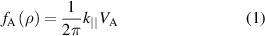
In experiments, rotational transform is varied by changing the current in one or more of the device's three coil systems. A diagram of the coil systems is shown at left in figure 1. In the shots of interest for this work, symmetric scans of coil current were conducted such that vacuum iota progressively shifted upward or downward. The right plot in figure 1 shows the coil current configurations and corresponding vacuum rotational transform (ιvac) during the scan.
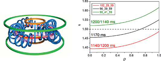
Figure 1. (Left) TJ-II coil system. The current in groups of three coils can be adjusted to vary the rotational transform profile: the circular coil (red), the helical coil (yellow), and the vertical field coils (green and orange). (Right) Vacuum iota profile tested in symmetric scan experiments. Numbers to the left of the slash indicate time instances for the profile shown in the upward scan scenario; to the right of the slash for the downward scan scenario. In the box, the coil current configurations are shown for each iota profile, where the current values correspond respectively to circular coil current, helical coil current, vertical field coil current,  _
_ _
_ . Reproduced courtesy of IAEA. Figure from [15]. Copyright (2014) IAEA.
Download figure:
Standard image High-resolution imageTJ-II is equipped with two neutral beam injectors, NBI1 and NBI2, known as co- and counter-injectors, which launch hydrogen (H) or deuterium (D) beam atoms into the plasma parallel and anti-parallel to the direction of the magnetic field, respectively. During the time slices of interest in the experiments considered in this paper, NBI1, the co-injector, was operating at PNBI = 0.57 MW [15].
The beam-driven Alfvénic activity resulting from the shifting up and down of the vacuum iota profile during the plasma operation was measured using a heavy ion beam probe (HIBP). Additional details about the functionality of HIBP can be found in [15, 17–20].
Our objective in the following sections will be to validate that a frequency-sweeping mode observed under NBI heating conditions in TJ-II symmetric discharges 27 804 and 27 806 with mode numbers m = 6, n = −9 can be accurately classified as an Alfvén cascade. Figure 2 shows the perturbations of the plasma density spectrogram for the aforementioned symmetric scan experiments. Note that the minimum value of the iota profile increases in time in discharge 27 804 and decreases in time in 27 806. The sweeping mode of interest is circled in yellow on both spectrograms.

Figure 2. Plasma density perturbation spectrograms for symmetric coil current scan experiments. Red arrows indicate observed frequency-sweeping Alfvén modes, and the yellow circles indicate the mode of interest for this work. Arrow labels indicate the calculated poloidal (m) and toroidal (n) mode numbers as well as radial mode locations (ρ) for each observed cascade mode (m/n@ρ). Note that the upper panel shows the time-directed experimental observation from TJ-II discharge 27 804, while the lower panel is a time-reversed reconstruction of the experimentally-observed mode evolution from TJ-II discharge 27 806. The modeling procedure that determined the mode numbers and birthplaces of the modes is described in detail in [15]. Reproduced courtesy of IAEA. Figure from [15]. Copyright (2014) IAEA.
Download figure:
Standard image High-resolution imageIts associated mode numbers and the minimum value of the rotational transform profile at the time of its observation were determined via an analysis procedure that was described in detail in [15]. Here we provide a brief summary of the analysis technique which closely follows that of [15].
Mode frequency is measured directly by HIBP and can be related to the wave vector of the observed mode by the Alfvén dispersion relation for plane waves in an infinite medium:
where  is the Alfvén velocity defined as,
Here, B is the magnetic field, µ0 is the vacuum permeability, ni is the plasma ion density, and mi is the ion mass.
The mode wave vector parallel to the magnetic field  is then determined in terms of the rotational transform ι and the mode poloidal and toroidal mode numbers, m and n respectively, as:
Finally, the true value of ι in the plasma, an unknown that appears in equation (3), must be related to its vacuum value, the experimental input parameter.
Note that the poloidal mode number m of each mode shown in figure 2 is determined by the slope of the line that best fits its downward-sweeping frequency as a function of ιmin (assuming that B and ni are held constant at the mode's radial location, which is fixed). The linear dependence can be seen explicitly by plugging equation (3) into equation (1).
Simulations with the equilibrium code VMEC (discussed in detail in section 3) were performed to find a linear function C that relates iota in the vacuum and in the plasma via the plasma current Ipl:

Here, the vacuum iota profile  and plasma current Ipl are known quantities and given as inputs to VMEC simulations. The output of VMEC is the modified iota profile
  as shown on the left hand side of equation (4). The resulting radial function C(ρ) and the VMEC outputs from which C(ρ) was constructed are shown in figure 3.

Figure 3. (Left) Modification of the vacuum iota profile (black) due to plasma current Ipl. Reproduced according to [15]. (Right) Radial function C which relates vacuum iota value with current-modified iota given by VMEC. as described in equation (4). Reproduced courtesy of IAEA. Figure from [15]. Copyright (2014) IAEA.
Download figure:
Standard image High-resolution imageIn the following sections we use the results of the analysis to constrain the parameters of our simulations; this includes the values of ιmin and the toroidal and poloidal mode numbers for the experimentally-observed modes. We consider the highest-fidelity measurement to be the mode frequency since it was directly measured rather than mathematically extrapolated.
3. Methodology
Modeling of the resulting frequency-sweeping Alfvén modes observed in the experiments described above was conducted using three codes: VMEC [21], a 3D equilibrium solver, STELLGAP [22], an Alfvén continuum solver, and AE3D [23], an Alfvén eigenmode solver, as was previously done in [24]. A visualization of the full workflow is shown is figure 4. In the following sections, each code and its respective role in the workflow is described in detail.

Figure 4. Simulation workflow with inputs shown in yellow, simulation software shown in blue, and outputs shown in green. Both STELLGAP and AE3D take the mode numbers of interest and plasma density profile as inputs, as well as the VMEC equilibrium.
Download figure:
Standard image High-resolution image3.1. VMEC
VMEC is an equilibrium solver built to model three-dimensional fusion devices. It uses a steepest descent method to find the minimum of the plasma potential energy function, which can be written as:
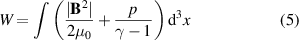
where B is the magnetic field, p is the pressure, γ is the adiabatic index and the integral is taken over the volume of the plasma. The resulting VMEC equilibrium file serves as the input to both the STELLGAP and AE3D solvers. Additional details about the VMEC code can be found in [21].
3.2. STELLGAP
STELLGAP [22] solves for the Alfvén continuum spectrum in a three-dimensional toroidal device. The continuum spectrum defines the frequencies, radial locations, and toroidal and poloidal mode numbers of shear Alfvén waves that are expected to be seen in a toroidal device with a particular equilibrium configuration (as defined by the input provided by VMEC).
To calculate the Alfvén continuum spectrum, STELLGAP solves the following equation in straight field line Boozer coordinates [25]:
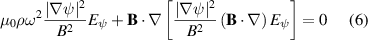
where ρ is the plasma mass density, and Eψ is the covariant ψ component of the electric field.
The resulting Alfvén continuum plots, showing the continuum frequency as a function of radius for the mode harmonics m and n involved, serve as a 'map' indicating the radial locations and frequencies of modes that are most likely to be driven unstable by high-energy particles. Compressibility effects can be optionally included in the calculation of these continuum plots in STELLGAP.
Modes are likely to be destabilized most easily by energetic particles when they are located in the gaps of the continuum, defined by a local minimum in a continuum line located above a local maximum in another continuum line. The frequencies of the modes in the continuum gaps do not cross the continuum lines and therefore avoid strong continuum damping, meaning they are weakly damped and easy to excite with energetic particles. Modes that are observed experimentally are generally expected to be those which are localized in the gaps of the continuum and in the following sections we will exploit this relationship to validate simulations against experiment. Note that in STELLGAP, due to the helicity in TJ-II (the sign of the iota profile, which in inputs is negative), toroidal mode numbers are reported as negative. All profiles shown in the following sections are plotted with iota positive.
3.3. AE3D
AE3D [23] calculates the eigenfrequencies and mode structures of shear Alfvén waves in a three-dimensional device. The governing equations of AE3D are the ideal MHD Ohm's law and the vorticity equation. When combined and simplified, they lead to the following eigenvalue problem:
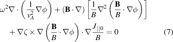
where  is the equilibrium parallel current, φ is the electrostatic potential, and ζ is the toroidal angle coordinate.
The resulting eigenfrequencies and mode structures can be used in conjunction with the continuum plot calculated by STELLGAP to identify which modes are located within gaps in the continuum, and therefore are most likely to be destabilized. AE3D does not include compressibility effects in its calculation of eigenfrequencies and mode structures.
4. Results
In this section, we first use the experimental results to calibrate the density profile for the discharge of interest. Once a reasonable density profile is determined, we use it as an input, along with the other experimental analysis results, to reconstruct the m = 6, n = −9 mode shown in figure 2. We also conduct a broader study on the concurrence of simulated gaps in the Alfvén continuum with the additional modes observed in experiments.
4.1. Density study
Recall that STELLGAP provides the locations of gaps in the Alfvén continuum for a given equilibrium configuration, and that modes that are most likely to be destabilized are those which are localized inside the gap region. Also note that simulation input parameters are constrained to those resulting from the experimental analysis that was described in section 2.
In this section, we study the localization of the reversed shear-induced gap region for various input plasma ion densities. The goal of this analysis is to calibrate the plasma ion mass density, which is a required input to STELLGAP and AE3D, taking into account the constraints on mode number, frequency and ιmin that were set by experimental analysis. While electron density is measured experimentally in TJ-II, ion density is not; therefore, the experimentally-measured frequencies will be used to calibrate ion density. The relationship between Alfvén frequency and ion density is described by equations (1) and (2).
Input iota profiles for this study are shown in figure 5 and a detailed discussion about the particular functional shape of these iota profiles will be provided in section 4.2.2. For now, they should be taken as an ansatz that is constrained by the values of ιmin that were predicted for the m = 6, n = −9 mode as shown in figure 2.
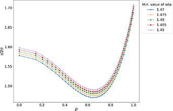
Figure 5. Non-monotonic ansatz iota profiles, where ρ is the square root of the normalized toroidal magnetic flux.
Download figure:
Standard image High-resolution imageFigure 6 shows the results of the study for three ion density profiles with varying on-axis values; the starting point for the shape of these profiles is the experimental electron density as given in [15]. In these results, the ion to proton mass ratio is fixed to 1 for simplicity. The results show that as the central ion density is decreased, the area of the reversed shear-induced gap generally becomes wider and shifts upward in frequency. The three central ion densities, distinguished by the areas shaded in grey, blue, and green, are overlaid against a sampling of points from the sweeping mode observed in TJ-II discharge 27 806. Recall that the perturbed density spectrogram data from which these points are sampled is shown in figure 2.
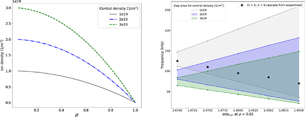
Figure 6. (Left) Input ion density profiles (Right) Location of gaps in the Alfvén continuum for each input ion density profile (shown with grey, blue, and green shading) compared with a sampling of points from experimentally-observed frequency sweeping Alfvén mode (shown as black stars).
Download figure:
Standard image High-resolution imageFigure 6 suggests that the true value of central ion density should fall somewhere between  (1/m3) and
  (1/m3), which is roughly in line with the experimentally-observed electron density [15]. The profile with central density
  (1/m3) is selected as the modeling input. It will be shown in section 4.2.2 that the error on the resulting modeled mode frequencies is relatively insensitive to variations in density.
It should be noted that although the locations of the gaps shown in figure 6 were calculated with the particular iota profile shape from figure 5, the resulting gap location is measured at ρ = 0.65 and is therefore specifically dependent on the iota profile's value at ρ = 0.65 and largely independent of its values elsewhere. Therefore, in calibrating the density, we have made no additional assumptions that would affect the output beyond assuming the results of the analysis described in section 2 and shown in figure 2 (specifically, the values of the x-axis as mapped to the frequency of the observed modes) to be correct.
4.2. Modeling the m = 6, n = −9 cascade
In the upcoming sections, we will attempt to reproduce the circled frequency-sweeping mode from figure 2 with two different types of ansatz rotational transform profiles: monotonically increasing and non-monotonic.
4.2.1. Monotonic iota profiles.
In this section, we demonstrate that the m = 6, n = −9 mode could not have been observed in a TJ-II discharge with a monotonic iota profile. Figure 7 shows ansatz iota profiles input to STELLGAP and AE3D. The functional shape of the profiles is identical to that of the TJ-II vacuum profile, and the profile is translated upward over five runs of the simulation to mimic the effect of dynamically changing the profile's minimum during a discharge.
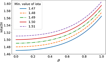
Figure 7. Monotonic ansatz iota profiles.
Download figure:
Standard image High-resolution imageThe continuum plot calculated in STELLGAP for each of the five iota profiles is shown in figure 8. Continuum lines are shown in blue, orange, green, red and purple, while individual eigenmodes with toroidal mode number n = −9 as calculated by AE3D are shown in black.

Figure 8. Continuum structures for monotonic iota profiles with minima at 1.47 (a), 1.48 (b), 1.49 (c), 1.50 (d) and 1.51 (e). Black lines represent the full width at half maximum of eigenmodes with toroidal mode number n = −9 calculated with AE3D.
Download figure:
Standard image High-resolution imageFrom these plots, we can observe that there are no eigenmodes (black lines) contained within any gap formed by the continuum lines (with the exception of a radially-extended gap mode around 280 kHz that appears when the minimum value of the iota profile is 1.49, but this mode is outside the frequency range of interest). We can conclude, therefore, that all of the modes with n = −9 for this rotational transform profile shape are subject to continuum damping and therefore unlikely to be destabilized.
This is an expected result since the input iota profiles are monotonic (continuously increasing with increasing radius) and therefore have normal shear. In order for reversed-shear Alfvén eigenmodes such as the ones suspected to have been observed in TJ-II discharge 27 804 to be present, the rotational transform profile must be non-monotonic [26]. Therefore, a monotonic iota profile shape can be ruled out.
4.2.2. Non-monotonic iota profiles.
In the previous section, we saw that the TJ-II vacuum iota profile, which is monotonically increasing with ρ, does not induce continuum structures that would accommodate the observation of the m = 6, n = −9 frequency-sweeping mode in discharge 27 804. This behavior is expected, as the modes of interest were observed during discharges with neutral beam injection, which can modify the vacuum iota profile. Neutral beam injection induces a plasma current  which, when assumed to be small, can be related to perturbations to the equilibrium in a linear way.
The left plot in figure 3 shows the modification of the vacuum iota profile (shown in black) due to various values of NBI-induced plasma current. These currents are of the same order as those computed by the ASCOT5 Monte Carlo orbit-following code for TJ-II [27].
Co-directional neutral beam injection induces a positive plasma current Ipl. From the result in figure 3, we see that in both cases with positive plasma current (Ipl =  ) the vacuum iota profile is modified to demonstrate strong magnetic shear.
Since we are modeling a discharge with positive plasma current, we create an ansatz iota profile with a strong degree of shear.
A second factor to consider when creating the ansatz iota profile for the strong shear non-monotonic case is the prediction of the location of the iota profile's minimum value. The methodology for arriving at the predicted value is described in detail in section 2. The result of the analysis was that the minimum value of the iota profile should occur at the radial location ρ = 0.65.
With both of these two factors accounted for, namely the profile's shear based on the experimental plasma current and the location of the profile's minimum based on the results of analysis from [15], we constructed the ansatz iota profiles shown in figure 5. These are the same profiles that were used as input for the density study discussed in section 4.1. Recall that in experiments in TJ-II, iota profile minimum can be varied linearly over a single shot via variation of the current in the device's magnetic coils. Therefore, each iota profile in the sequence can be thought of as a single snapshot in time of the evolution of the Alfvénic activity during the discharge.
Each of the five iota profiles shown in figure 5 were run through VMEC, STELLGAP and AE3D as described in section 3. In figure 9, results from both STELLGAP and AE3D are shown for each profile.

Figure 9. Continuum structures for non-monotonic iota profiles with minima labeled individually. The n = −9 continuum line is shown both with (pink) and without (green) sound coupling effects included. The black horizontal line on each plot represents the full width at half maximum of a mode with poloidal and toroidal mode numbers m = 6 and n = −9, respectively. The mode frequencies, radial locations, and widths are calculated by the AE3D code.
Download figure:
Standard image High-resolution imageThe colored lines on each plot represent the Alfvénic continuum structure for the n = −1 mode family to which the n = −9 mode belongs (cf table 1). Recall that the Alfvén continuum structure indicates the expected frequencies and radial locations of Alfvén waves for a discharge with the respective iota profile. The color of each line indicates the mode's toroidal mode number (n).
Table 1. Table showing input toroidal (n) and poloidal (m) mode numbers for each mode family.
| Family 1 | Family 2 | Family 3 | Family 4 |
|---|---|---|---|
| n = −1; m = 1–5 | n = −2; m = 1–5 | n = −3; m = 1–5 | n = −4; m = 1–5 |
| n = −5; m = 3–8 | n = −6; m = 3–8 | n = −7; m = 3–8 | n = −8; m = 3–8 |
| n = −9; m = 5–15 | n = −10; m = 5–15 | n = −11; m = 5–15 | n = −12; m = 5-15 |
| n = −13; m = 7–17 | n = −14; m = 7–17 | n = −15; m = 7–17 | n = −16; m = 7-17 |
| n = −17; m = 9–27 | n = −18; m = 9–27 | n = −19; m = 9–27 | n = −20; m = 9-27 |
On each of these plots, there is a gap in the continuum structure localized approximately at ρ = 0.65, formed by the local minimum of the n = −13 continuum line located above the local maximum of the n = −9 continuum line. Recall that the minimum value of each iota profile, or the location of the reversal of the profile's magnetic shear, is also at ρ = 0.65. Based on these coincident radial locations, we conclude that this gap is a reversed-shear induced gap in the Alfvén continuum.
The black horizontal line on each plot represents the full width at half maximum for a mode that falls inside the aforementioned gap as calculated by AE3D, and the full mode structures for each time slice are shown in figure 10. Recall from section 3.2 that modes inside the gaps of the Alfvén continuum are the most likely to be destabilized, and therefore the ones most likely to be observed in experiments.
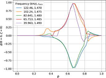
Figure 10. Mode structures associated with each iota profile (or time slice) shown in figure 9. Mode frequencies and associated values of the minimum of the iota profile are shown in the legend. The frequency for each mode corresponds to the y-value of each of the black horizontal lines in figure 9.
Download figure:
Standard image High-resolution imageEach plot in figure 9 also includes the modified n = −9 continuum line when compressibility effects, or coupling to sound waves, are included in the simulations [28]. The effect of including compressibility is to shift the continuum line upward in frequency, as demonstrated by the comparison between the green and pink continuum lines. The difference between the maximum frequency of the compressible and incompressible continuum lines increases with increasing value of ιmin, reaching a maximum of 30 kHz of separation in the ιmin = 1.490 case. In the incompressible case, the mode frequency calculated by AE3D moves downward in frequency along with the peak of the n = −9 continuum line (green). It is inferred that the same would be true of the relationship between the n = −9 compressible continuum line (pink) and the sound-coupled mode frequency, resulting in an overall upward shift in frequency of the mode at each value of ιmin. Given that AE3D does not include compressibility effects, it cannot be used to confirm the above hypothesis. For such an assessment, a code such as CAS3D could be used instead [29].
As the minimum value of the iota profile sweeps linearly upward, the frequency of the mode sweeps linearly downward, indicating that these modes can, in fact, be identified as reversed-shear Alfvén eigenmodes. A plot of the frequency of the mode versus the minimum value of the iota profile for which it was observed is shown in figure 11. Error bars are included, showing the calculated error in frequency when a relatively small error of ±0.005 in iota and ±10% in density are assumed. The error of ±0.005 on iota was chosen from the full measured error range of 0.004–0.037 in iota as shown in figure 11 of [15]. Each of these two errors are considered independent from one another, and are propagated through equations (1)–(3) via addition in quadrature. The vast majority ( 90%) of the resulting error on the frequency value is due to the uncertainty in iota.

Figure 11. Simulation results shown in black overlaid with zoomed in experimental spectrogram from figure 2. Each black simulation point has the frequency value of the black horizontal lines shown in figure 9. Error bars assume ±10% error in density and ±0.005 error in iota.
Download figure:
Standard image High-resolution imageWe see that simulations in which the non-monotonic profile minimum is varied as predicted by analysis give decent agreement with experimental observations. For the first four simulated points, the measured mode falls comfortably within the simulation's error bars. The fifth point, at ιmin = 1.490, captures the second displayed measured mode within its error bar range when an error of ±0.01 in iota is considered.
We expect that the comparison between the experimental and computed mode frequencies would further improve by taking into account the compressibility effects that are not included in the AE3D results in figure 11. We expect that taking into account these effects would result in an upward shift of the calculated mode frequency with the magnitude of shift increasing with the minimum iota, as suggested by the STELLGAP results for the n = −9 continuum line shown in figure 9.
As compared with the monotonic profiles in the previous section, non-monotonic profiles can produce frequency-sweeping Alfvén cascades, which supports theoretical predictions.
4.3. Additional cascades
As an extension of the study beyond the m = 6, n = −9 mode in the ιmin range of 1.47–1.49, we have carried out simulations for a wider ιmin range of 1.42–1.55 which is similar to the range explored experimentally (cf figure 2). Our objective in this extended study is to investigate whether additional cascades beyond the m = 6, n = −9 mode could occur according to modeling and, if so, with what mode numbers and frequencies.
First, STELLGAP simulations were carried out where the non-monotonic iota profiles considered in section 4.2.2 were shifted up or down to match the predicted ιmin values from the analysis results shown in figure 2. In these simulations, four mode families with input toroidal and poloidal mode numbers as shown in table 1 were considered. Moreover, the ιmin range of 1.42–1.55 was divided in four parts and in each part, the family of input toroidal mode numbers was selected to coincide with the family of the toroidal mode number n given by the post-experiment analysis in that ιmin range (deduced mode numbers m n−1 are indicated by the labels of the red arrows in figure 2). Consequently, the mode families 3, 2, 1 and 4 were considered in the ιmin range of 1.445–1.465, 1.46–1.475, 1.47–1.49 and 1.54–1.55 respectively, while all other variables including the plasma ion density and the location of the minimum of the iota profile (ρ = 0.65), were held constant.
Note that this approach results in a simplification of the experimental situation for which the post-experiment analysis [15] suggested that the minimum value of the iota profile evolved radially outward from a minimum of ρ = 0.2 to a maximum of ρ = 0.8 during the time interval shown in figure 2. The radial evolution of the minimum value of the iota profile is neglected in this work to limit the number of independent variables in each simulation, though it could be considered in future work.
The resulting locations of gaps in the Alfvén continuum spectrum as a function of the minimum of the iota profile are shown in figures 12–15 for the first sweeping mode for each mode number family.
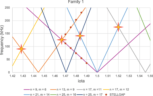
Figure 12. Location of gaps in the Alfvén continuum spectrum of mode family 1 for various values of the minimum of the iota profile indicated by the minimum and maximum of the reversed shear-induced gap in the Alfvén continuum as given by STELLGAP (red dots) and the Alfvén frequency as given by  kHz (colored lines). Note that STELLGAP simulations were run in search of the specific mode numbers and locations in ιmin
that are indicated in figure 2. In this case, the search was conducted for mode family 1 in the range 1.47–1.49 in ιmin (see text for details). The stars indicate locations where a continuum line n and another continuum line n + 4 coincide in frequency. These points represent locations in the frequency-ιmin space where a downward-sweeping cascade mode could appear.
kHz (colored lines). Note that STELLGAP simulations were run in search of the specific mode numbers and locations in ιmin
that are indicated in figure 2. In this case, the search was conducted for mode family 1 in the range 1.47–1.49 in ιmin (see text for details). The stars indicate locations where a continuum line n and another continuum line n + 4 coincide in frequency. These points represent locations in the frequency-ιmin space where a downward-sweeping cascade mode could appear.
Download figure:
Standard image High-resolution image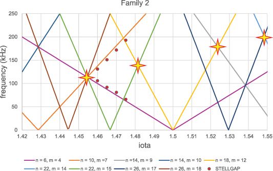
Figure 13. As in figure 12 but for mode family 2. STELLGAP points are the result of a search for mode family 2 only in the range 1.46–1.475.
Download figure:
Standard image High-resolution image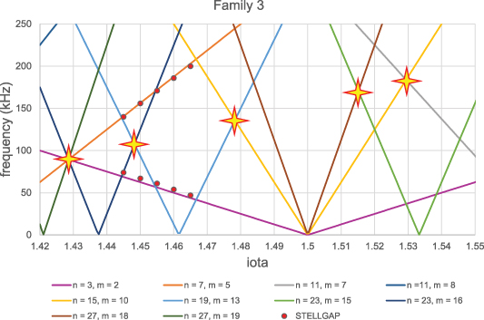
Figure 14. As in figures 12 and 13 but for mode family 3. STELLGAP points are the result of a search for mode family 3 only in the range 1.445–1.465.
Download figure:
Standard image High-resolution image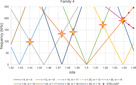
Figure 15. As in figures 12–14 but for mode family 4. STELLGAP points are the result of a search for mode family 4 only in the range 1.54–1.55.
Download figure:
Standard image High-resolution image
In their frequency and ιmin values, the gap locations could roughly accommodate some of the experimentally-observed modes shown in figure 2 (recall that the locations of destabilized cascade modes correspond to the location of gaps in the Alfvén continuum).
In order to corroborate the STELLGAP results shown in figures 12–15, a simple analytical model was constructed. Combining equations (1)–(3), we find that the Alfvén frequency for a mode with a toroidal mode number n and poloidal mode number m can be written as

where C is a constant and ι is the minimum value of the iota profile. The constant C = 625 kHz was determined using STELLGAP results with  = 75 kHz for the m = 6, n = 9 mode at ι = 1.48 (cf figure 12). The allowed frequencies of Alfvén modes were then calculated with this simple formula for seven toroidal mode numbers in each family shown in table 1. The resulting modes with frequency below 250 kHz in the iota range of 1.42–1.55 are shown in figures 12–15 together with the STELLGAP results.
Comparing the gap boundaries calculated by STELLGAP for the first sweeping mode for each mode number family with the lines calculated by the simple analytical model shown in figures 12–15, we see that the analytical model reproduces STELLGAP points very well. The points marked with stars in figures 12–15 indicate locations where a continuum line n and another continuum line n + 4 coincide in frequency. These points represent locations in the frequency-ιmin space where a downward-sweeping cascade mode could appear. The interpretation of these points as the locations where cascades could be instantiated is supported by the results from STELLGAP and AE3D. According to STELLGAP and AE3D, it is in the gap of the maximum and minimum of the n = 9 and n = 13 continuum lines, respectively, that the observed n = 9, m = 6 mode appears. Note also that the n = 9, m = 6 mode follows closely the maximum of the n = 9 continuum line as the minimum value of iota increases (cf figure 9).
When there is a clear observation that the measured frequency reaches a minimum, as in figure 2, it can be used to determine the corresponding rational iota value. Figure 12 demonstrates that the n = 9, m = 6 mode is expected to reach its minimum value in frequency at the rational iota point of 1.5. The measured mode shown in figure 2 appears to reach its minimum at ιmin = 1.51. This suggests that the true error on the experimental measurement of iota is likely 0.01, which is included in the aforementioned full measured error range of 0.004–0.037 as shown in figure 11 of [15].
The simple analytical model correctly predicts the points where each of the four modes identified in figure 2 are instantiated. It also reproduces a trend seen in experimental results, namely that the frequency at which the downward-sweeping mode is instantiated increases with increasing ιmin. It also suggests additional modes which could explain the experimentally-observed modes in figure 2 which were not identified by the post-experiment analysis reported in [15], though it should be noted that the existence of a gap in the Alfvén continuum spectrum does not directly imply the existence of a cascade in that frequency range.
5. Conclusions
A validation study was conducted which aimed to computationally model frequency-sweeping Alfvén modes observed during experiments in the TJ-II stellarator. In the experiments, variations in coil current induced shifting of the minimum of the iota profile which led to Alfvénic activity suspected to be of an RSAE-like nature [15]. In this work, we showed that the iota profile for such a discharge could not have been purely monotonic, as simulations with monotonic iota profiles do not produce any modes that are localized in gaps in the Alfvén continuum. With non-monotonic iota profiles, however, a mode whose toroidal and poloidal mode numbers match those of the mode of interest observed in TJ-II is shown to sweep downward in frequency as the minimum value of the iota profile is shifted upward. Based on this behavior, the simulated modes can be identified as Alfvén cascades. We have also shown that with these non-monotonic iota profiles, gaps appear in the Alfvén continuum whose frequencies and minimum iota values roughly accommodate the cascade modes seen in experiments.
Acknowledgment
We acknowledge financial support from the FusionCAT Project (001-P-001722) co-financed by the European Union Regional Development Fund within the framework of the ERDF Operation Program of Catalonia 2014–2020 with a grant of 50% of total cost eligible. We also acknowledge the collaboration and support of J.L. Depablos, A. Cappa, C. Hidalgo, K. McCarthy, F. Medina and the whole TJ-II team.