

Abstract
We propose a model of network growth in which the network is co-evolving together with the dynamics of a quantum mechanical system, namely a quantum walk taking place over the network. The model naturally generalizes the Barabási–Albert model of preferential attachment and it has a rich set of tunable parameters, such as the initial conditions of the dynamics or the interaction of the system with its environment. We show that the model produces networks with two-modal power-law degree distributions, super-hubs, finite clustering coefficient, small-world behaviour and non-trivial degree–degree correlations.
Export citation and abstract BibTeX RIS
Models of graph growth are important for studying and simulating the behaviour of a large variety of real-world phenomena and for the in silico construction of networks with given properties. Growth processes occur ubiquitously in social systems, technology, and nature. See, for example [1]–[3], for overviews on complex networks growth. Among the most extensively studied models of network growth are those based on preferential attachment—or 'the rich get richer' scheme—together with its many variations [4]. Predating networks science, the basic idea behind preferential attachment goes back to the 1920s and the work of the statistician Yule [5]. The setup usually consists of two ingredients: an iterative process in which new nodes are sequentially added to an existing graph; and a mechanism for choosing the neighbours of newly arrived nodes. Only when the preference on the neighbours is a linear function of the degrees of the nodes, then the degree distribution of the growing graph turns out to be a power-law, as those observed in the majority of real-world complex networks. The literature contains many variants of preferential attachment, respectively defined by local rules, fitness, redirection, copying, substructures, games, geometry, etc [6].
We are interested in generalizing the classical preferential attachment model, in which the choice of the nodes to link to is specified by the dynamics of random walks [7]. The original idea, illustrated in [8]–[10], is simple. Imagine a walker moving along the edges of a graph. At a given node, the walker chooses to stay where it is or to move to one of the neighbouring nodes with a fixed but arbitrary probability. If we wait long enough, the probability that the walker is at a specific node is proportional to the number of its neighbours: this probability converges towards a unique stationary distribution and is independent of the starting node—a fundamental property in algorithmic applications of Markov chains [11, 12]. Once we are close enough to the stationary distribution, we add a new node to the graph, and choose its neighbours according to the occupation probability distribution induced by the walker. If we keep adding nodes in this way, we eventually grow a graph whose degree distribution follows a power-law. When the walker makes an unbiased choice at each node, i.e. when the stationary occupation probability of the walker at node i is a linear function of the degree of i, then this mechanism produces exactly the Barabási–Albert (BA) random graph [4], which is the most widely studied outcome of preferential attachment so far.
Graph growth indeed fits into a larger picture, namely the study of dynamical graphs, i.e., graphs changing in time. This is a direction that is currently generating interest as a natural development of static network theory (see [13] is a recent review). Letting the structure of a graph co-evolve together with a dynamical process is a particularly appealing and well-motivated idea. In particular, the existence or activity of a node and the strength of a link can be time dependent on the state of a dynamical process taking place on the graph. For instance, if the nodes of a graph represent individuals having an opinion which changes over time according to a certain rule, and the links stand for friendship among nodes, then the existence and strength of each link can change over time as a function of the difference of opinion between adjacent nodes. People usually tend to remain linked with neighbours who share similar opinions, and to sever links to other individuals having different opinions. In this case the structure of the network depends on the distribution of opinions and, on the other hand, the opinion dynamics depends on the actual connection pattern. In a single word, the network and the opinion formation process are co-evolving. Opinion formation is of course only a very specific example of a process able to drive the evolution of a network. Many other models of networks co-evolving with synchronization [14], diffusion [15], and voter models [16, 17] have been discussed in the past decade (see also [18]).
Networks seen as states of a quantum mechanical system co-evolving together with a classical process have been proposed to explore the role of emergence in approaches to discrete quantum gravity [19]. Networks whose edges correspond to bipartite states—essentially certain circuits with two-qubit gates—have been studied in relation to entanglement distribution [20].
With the aim of designing a new methodology to grow complex networks, we ask the following question: what happens when we consider a graph whose growth depends on the state of a quantum mechanical system? In particular, we are interested in replacing the random walk dynamics, which produces the BA random graph, with a quantum dynamics. At each step of the growth process, the neighbours of the newly added node are chosen by observing the state of the quantum system—by using a standard (von Neumann) measurement. We have the co-evolution of two processes: each step of the graph growth process depends on a quantum dynamics and, conversely, the dynamics takes place in a phase space (the graph) modified during the growth.
Quantum walks have been extensively studied in the past forty years: a continuous version is discussed in [21] and dates back to 1964; a discrete version was introduced in the 1990s [22]. During the past decade, quantum walks have acquired an important role in the context of quantum computation as a methodology for designing algorithms [23, 24]. Quantum walks are also essential in modelling quantum buses for the transfer of information in nanodevices. The dynamics of an exciton in a spin chain or an arbitrarily coupled spin system is modelled by a coherent quantum walk [25, 26]. Additionally, the transport of energy in large molecular complexes has been explained using a class of quantum walks whose evolution is assisted by interactions of the system with a noisy environment [27]. Very recently, quantum walks have also been employed for the characterization of complex networks [28, 29].
The quantum walker, like the classical (i.e., random) one, induces a probability distribution on the nodes of a graph. However, the distribution is obtained by measuring the state of the system at a given time. In quantum mechanics, the state (of a closed system) is identified with a unit vector in a complex phase space, with probabilities substituted by amplitudes. A major property of quantum walks is the existence of interference effects during the dynamics. Once the position of the quantum walker is measured, the corresponding probability distribution is the result of an interference pattern. Notably, the distribution does not converge in time because the evolution of a quantum mechanical system is completely reversible [22, 30]. The dynamics can be periodic, or quasi-periodic, but there is no convergence unless we take a time-average [31]—or we stop the evolution at a given time. Interference is one of the ingredients that permits algorithms of good performance to be designed [32] and is also responsible of many counterintuitive behaviours of quantum systems. For instance, transporting a packet of information from one node to another node without error, even if routed 'randomly' through the graph—a phenomenon called perfect state transfer [26]; or reaching far away nodes with an average probability that is exponentially higher than that for the classical analogue [33]. It is also remarkable that quantum walks have been successfully implemented through various experimental schemes involving light or matter [34]–[36].
Here we work with continuous-time quantum walks (CTQW) [37]. In these processes the matrix defining network links is interpreted as the system Hamiltonian: this is the operator corresponding to the total energy of the system. The Hamiltonian specifies the interactions between the particles associated with the nodes in terms of coupling strengths. CTQWs are reversible by definition, since the dynamics is governed by the Schrödinger equation. (A formal definition is given in the appendix.)
What can we say about graphs whose growth depends on the state of quantum walks? Do they have structural properties comparable to those of the BA random graph? The time at which the measurement is performed (i.e. the time at which the walk is stopped) drastically influences the distribution of attachment probabilities; moreover, the choice of the node from which the walk is started may affect the occupation probability distribution measured at a certain time. These facts reflect the much richer behaviour of quantum walks with respect to random walks. In order to associate a probability distribution to the CTQW, we consider the time-average of all distributions obtained by running the walk for a given time. At each step of the iteration, we could choose the distribution obtained by stopping the walk at a time determined by a function of the number of nodes. We choose here (arbitrarily) to run the walk for an infinite time—this is like stopping the walk at a random time and it looks like a good choice for exploring the general idea. The time length of each walk is in fact a tunable parameter, differently from the classical BA model in which the growth depends on the long-time dynamics of the walk.
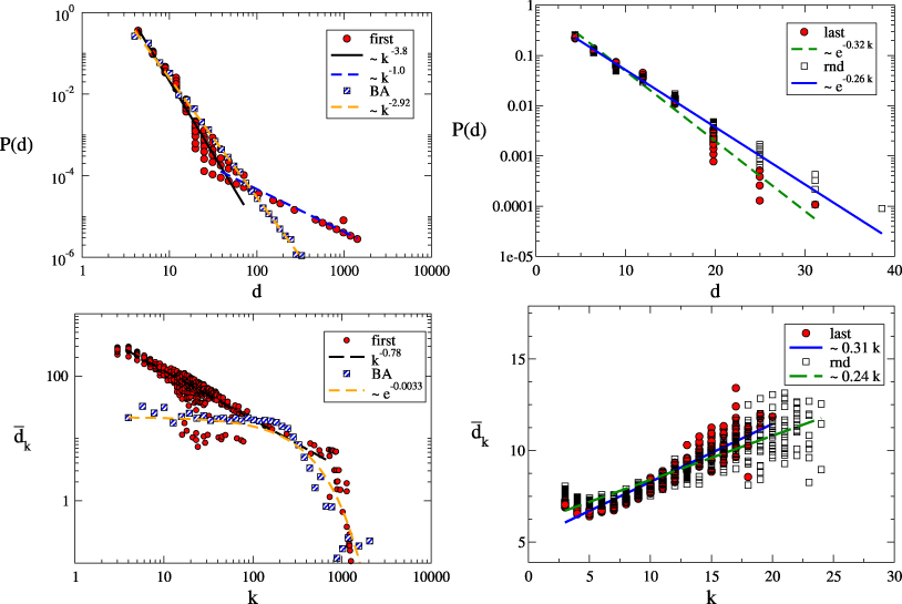
Figure 1. The structural properties of the final network depend heavily on the choice of the starting node for the quantum walks. If the walks starts from the node used to seed the growth process (upper left panel), we get a two-mode power-law degree distribution. In this case there is a non-negligible probability of forming a super-hub which condenses a large fraction of the edges of the network. Also, the final network has pronounced disassortative degree–degree correlations (lower left panel). Conversely, if the walk starts from the lastly added node, or from a randomly selected one, then the degree distribution of the final network is instead exponential (upper right panel). In this case there are slightly assortative degree–degree correlations (lower right panel). The results are based on 20 realizations, with N = 3000 nodes and K = 9000 edges for each scenario.
Download figure:
Standard image High-resolution imageWe consider here three alternatives for the starting node used to seed the quantum walk: (a) the walks always start from the initial node, i.e. the node added at the first step of the graph growing iteration; (b) the walks always start from the node added at the last step; (c) at each step, the starting node is chosen at random—of course, we could consider any probability distribution on the set of existing nodes. Since the growth is driven by the quantum walk, which effectively acts as a 'controller', we expect different asymptotic distributions. On the one hand, obtaining the time-average of a CTQW is a tractable problem; but on the other hand, predicting the properties of our growing graphs is a difficult one because the time-average has erratic behaviour [38]. Presenting an analytic treatment of the asymptotics remains an open problem.
In figure 1 we report the results of numerical simulations of the model with different initial conditions. We have constructed networks with N = 3000 nodes and K = 9000 links. We observe that different choices of the starting node produce graphs with different structural properties. For selection (a), the final graph is characterized by a two-mode power-law degree distribution (upper left panel) and has super-hubs, i.e. nodes with degree of the same order of the total number of nodes. Such exceptionally highly connected nodes are usually among the oldest ones, i.e. the nodes added in the very first steps of the iteration. Each super-hub turns out to be incident with up to 30% of the total number of edges in the final graph. This condensation phenomenon is indeed observed in real communication and information networks, including the Internet and the World Wide Web, and in biological networks [3]. Notice that the degree distribution obtained in (a) is different from that obtained for the BA random graph shown in the same panel. An obvious by-product of the existence of a super-hub is that the average length of the shortest paths between the nodes is much smaller than the one observed in the Erdős–Renyi (ER) and BA random graphs of the same size, as highlighted below.
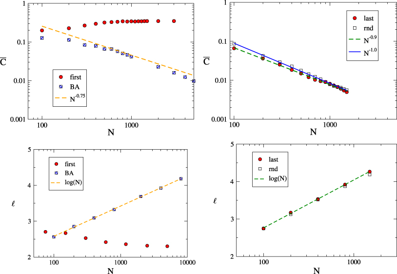
Figure 2. Scaling of the average clustering coefficient (top) and characteristic path length (bottom) for CTQW-based growths. When walks start from the first node (left panels) the average clustering coefficient increases with the network order N until it reaches a plateau around  , while the characteristic path length decreases with N. If the walk starts from the last node or from a randomly selected one, then the clustering coefficient decreases over time as N−1, while the characteristic path length increases logarithmically with N.
Download figure:
Standard image High-resolution image
The final graph also exhibits a surprisingly high local cohesion. This corresponds to a relatively high value of the average clustering coefficient (denoted by  ), a property which is extensively found in real networks but is rarely reproduced in models of random graphs without introducing artificial ingredients. Another remarkable property is the presence of pronounced disassortative degree–degree correlations: the average degree
  of the neighbours of a node with degree k depends on k and decreases as a power-law,
  , with ν ≃− 0.8. The existence of disassortative degree–degree correlations is partially due to the fact that the degree distributions of the resulting graphs do not have a structural cut-off [39], so that the average degree of the neighbours for a substantial fraction of the nodes (i.e., those nodes which share an edge with the super-hub) is dominated by the degree of the super-hub. For comparison, we report in the same panel the value of
  for the BA random graph, which is practically independent of k, except for the boundary effects observed for high values of k.
Conversely, for selections of type (b) and (c), namely when the walk starts either from a randomly chosen node or from the last node, we obtain exponential degree distributions and small assortative degree–degree correlations (upper right and lower right panels, respectively). In this case, the degrees appear to be more homogeneous: the final graph has neither hubs nor super-hubs, it exhibits a negligible clustering coefficient and an average shortest path length (denoted by ℓ) comparable to that of an ER or a BA random graph with an equal number of nodes.
For instance, in ER and BA random graphs with N = 3000 nodes, such as those reported in figure 1, ℓ ≃ 4.29,  and ℓ ≃ 2.54,
  , respectively. Instead, in the case of CTQW-based growth, when the walks start from the seed node of the growth process, then the final graph exhibits a clustering coefficient
  , which is much higher than expected in a random graph, and a considerably smaller average path length ℓ ≃ 2.41, which is in turn smaller than those observed in ER and BA graphs of the same size and order. Therefore, graphs grown with this method are small worlds [40]. When the walks start from the last node, we have ℓ ≃ 4.26 and
  , which are values comparable to those observed in ER and BA graphs. Choosing the starting node at random does not seem to result in a significant difference: ℓ ≃ 4.18 and
  . In figure 2 we study the scaling of
  and of the average shortest path length ℓ with the network order N. We compare CTQW-based networks with BA scale-free graphs. Notice that, while the average clustering coefficient of a BA network decreases as N−3/4 [41], in CTQW-based growth with walks starting from the seed node,
  grows with N until it reaches a plateau around
  . Similarly, the average path length decreases with N, until it reaches a plateau around ℓ ≃ 2.3. These scaling behaviours are mainly due to the condensation of edges around super-hubs, which favours the creation of triangles and contributes to lower the average path length. As we see from the two right panels of figure 2, if the walks are started from the last node or from a randomly selected one, then the scalings of
  and ℓ are comparable to those observed in classical random graphs. The notions of assortative/disassortative degree–degree correlations, clustering coefficient and average shortest path length are standard in the toolbox of network theory. We recall these definitions in the appendix.
As mentioned above, CTQWs have reversible dynamics and the (von Neumann) entropy of any state during the evolution is zero. The dynamics changes if we include an interaction between the system and its environment. This introduces decoherence, a phenomenon responsible for the quantum-to-classical transition. Due to decoherence effects, the system becomes thermodynamically irreversible. There are various ways to model decoherence in quantum walks, for example, by monitoring the evolution of the system at a certain rate. The non-zero probability of performing measurements can be interpreted as a weak coupling between the quantum system and a Markovian environment (see [42] for a detailed survey of the topic). Generally, when we increase the decoherence rate, the quantum features disappear and, after a critical point, the behaviour of the system becomes classical. Thus, in the case of a fully decohered quantum walk, we are able to recover the familiar preferential attachment induced by classical random walks [4, 8]—a random walk can be also obtained algorithmically from a CTQW [43]. We can interpolate between these two modes by turning the level of decoherence up or down [44, 45]. For very high decoherence rates, the system will tend to remain in the initial state due to the quantum Zeno effect [46]. This phenomenon can arguably be used to influence the behaviour of the degree sequence by choosing the node from which each walk is started.
The purpose of the first papers on quantum walks, written in the context of quantum computing, was to determine whether these dynamics could be used in algorithmic applications. Indeed, since then, quantum walks have been very important as a tool to design new quantum algorithms [23, 31, 32], in both the continuous and the discrete setting. Two reasons are behind this fact: quantum walks permit, in some cases, faster convergence towards the limiting distribution than their classical analogues; the limiting distribution—in the ways that this is defined to avoid the lack of convergence due to unitarity—often takes the shape of interference patterns that are far away from uniform. Interference is responsible for peaks in the distribution which may turn out to be useful to sample specific vertices. Therefore, we can use quantum walks to generate exotic probability distributions with the potential of highlighting certain subgraphs. The most successful application of this phenomenon is, arguably, perfect state transfer, where the state of a single qubit on a network of quantum spins can be transferred with complete fidelity between two particles, or periodicity, where after a given time the whole network is again in a past state. Such a behaviour gives routing without local control and it cannot be found in classical random walks. With respect to the topic of the present paper, faster convergence would imply a more efficient process to simulate network growth. Of course, the process is quantum and requires a physical implementation. In addition, quantum walks have many tunable parameters, as we have seen above. By changing, sometimes even minimally, the initial conditions and transition amplitudes, we can modify a walk in substantial ways, and this freedom in choosing the parameters allows the growth of networks with different properties, something which is not classically available unless we steer each classical walk with extra local rules.
In this paper we have defined a single model and studied some of its basic features, but investigating the whole potential of quantum walks in network growth is a completely open direction of research. Determining the correlation between dynamical parameters and network properties is a new, unorthodox problem at the interplay of algebraic graph theory and eigensystem analysis for unitary matrices. Also, we have not considered Anderson localization, partial decoherence, and noisy evolution. These are all physical features that can be naturally introduced into models of network growth, and that are well motivated by the available background. The effect of such features on networks may, in turn, suggest novel physical insight. Another extension of the model could be in the same spirit of [47]. The probability of attachment is determined by the outcome of a process external to the network. In our setting, the process could be a quantum walk on the integers, with the zero on the number line corresponding to the first vertex of the growth. What type of networks are grown when sampling from the interference pattern of the walk? Again, by the behaviour of the amplitudes and a specific tuning of the parameters, we should obtain networks without a known unified classical method of construction. This is left for further study.
Acknowledgments
Part of this work has been done at the Kavli Royal Society International Scientific Centre during the workshop 'Function Prediction in Complex Networks' (May 28–29 2012). We are grateful to Gorjan Alagic, Andrew Childs, Vivien Kendon and Andrea Torsello, for useful discussion.
Appendix:
A.1. Quantum walks
A graph G = (V,E) is an ordered pair, where V(G) is a set whose elements are called nodes and E(G)⊆V(G) × V(G) is a set whose elements are called edges. Since we consider graphs growing over time, we denote by Gt = (V,E) the configuration of nodes and edges at iteration t. Notice that the time of the growth is a discrete variable which is increased by one for each new node added to the graph. Consequently, the graph Gt has exactly t nodes. The lazy walk matrix on a graph at time t, Gt = (V,E), is (or, equivalently, is induced by) , where It is the t × t identity matrix, A(Gt) and Δ(Gt) are the adjacency matrix and the degree matrix of Gt, respectively. Recall that [A(Gt)]i,j = 1 if {vi,vj}∈E(Gt) and [A(Gt)]i,j = 0 otherwise; [Δ(Gt)]i,j = δi,jd(vi), where d(vi):=|{vj: {vi,vj}∈E(Gt)}| is the degree of vi, and δi,j is the Kronecker delta. The rule of the walk on the t-iteration graph is
  , where
  is an element of the standard basis of Rt and
  . The matrix Ws(Gt) induces a distribution on the nodes of Gt. The j-point of the distribution corresponds to the probability of finding the walker at node vj at time s if the walk started at time 0 from node vi. Thus, the probability is
 ![$\mathbb{P}\left [i\rightarrow j,s\right ]=\langle {\overrightarrow {v}}_{j},{\overrightarrow {\psi }}_{s}\rangle $](https://content.cld.iop.org/journals/1742-5468/2013/08/P08016/revision1/jstat482661ieqn78.gif) .
.
Independently of the initial state, the lazy walk W(Gt) converges to a unique stationary (probability) distribution π(Gt), such that [π(Gt)]i = d(vi)/2|E(Gt)|, for each i = 1,...,t (see, e.g., [48]). Convergence is guaranteed by the stochasticity of W(Gt) and by the fact that there is a non-zero probability for the walker to remain at each node. The rate of convergence depends on the spectral gap of the adjacency matrix.
The stationary distribution of a lazy walk on G2 is clearly the vector ![$\boldsymbol{\pi}\left ({G}_{2}\right )=\frac{1}{2}\left [1,1\right ]^{\mathrm{T}}$](https://content.cld.iop.org/journals/1742-5468/2013/08/P08016/revision1/jstat482661ieqn85.gif) . When adding v3 to G2, we define
. When adding v3 to G2, we define ![$\mathbb{P}\left [\{ {v}_{1},{v}_{3}\} \in E\left ({G}_{3}\right )\right ]=\mathbb{P}\left [\{ {v}_{2},{v}_{3}\} \in E\left ({G}_{3}\right )\right ]=\frac{1}{2}$](https://content.cld.iop.org/journals/1742-5468/2013/08/P08016/revision1/jstat482661ieqn88.gif) , which follows from π(G2). More generally, when adding a node vt+1 to Gt, we attach vt+1 to m ≥ 1 nodes in Gt, so that the probability of attaching vt+1 to vi reads P[{vt+1,vi}∈E(Gt+1)] = [π(Gt)]i. The parameter m is fixed but arbitrary. It is important to remark that m is not necessarily the degree of node vt+1 at the end of the growth process, which may occur at a time T > t. When m > 1 we usually start the growth from a (connected) graph Gm.
, which follows from π(G2). More generally, when adding a node vt+1 to Gt, we attach vt+1 to m ≥ 1 nodes in Gt, so that the probability of attaching vt+1 to vi reads P[{vt+1,vi}∈E(Gt+1)] = [π(Gt)]i. The parameter m is fixed but arbitrary. It is important to remark that m is not necessarily the degree of node vt+1 at the end of the growth process, which may occur at a time T > t. When m > 1 we usually start the growth from a (connected) graph Gm.
This mechanism constructs exactly the scale-free graphs for the original version of the Barabási–Albert (BA) model [4]. In the BA model, bypassing the walk, a node vt+1 of degree m is added at time t. The probability that vt+1 is adjacent to vi is in fact P[{vt+1,vi}∈E(Gt+1)] = [π(Gt)]i = d(vi)/2|E(Gt)|, which is exactly the stationary probability of finding a lazy random walker in Gt at node vi.
By generalizing the above picture, given a graph on t nodes, Gt, we define a unitary matrix U(s,t) = e−iA(Gt)s, where s∈R+. Unitary means that U(s,t)U†(s,t) = U†(s,t)U(s,t) = I, where I is the identity matrix and U†(s,t) is the adjoint of U(s,t). In this case the dynamics is reversible/non-dissipative because of unitarity. The matrix U(s,t) defines a continuous-time quantum walk (CTQW) on Gt [23]. The rule of the CTQW at the t-iteration is U(s,t)|vi〉⟼|ψs〉, where |vi〉 is an element of the standard basis of a formal Hilbert space  ≅ Ct and |ψs〉∈. The Dirac notation tells us that |||ψs〉|| = 1. The probability that at time s the walker visits a node vj starting in a node vi is P[i → j,s] = |[U(s,t)]i,j|2. This probability is obtained by a projective measurement on |ψs〉: P[i → j,s] = |〈vj|ψs〉|2. The vector (or ray) |ψs〉 contains the amplitudes associated to each element of the standard basis. The measurement transforms amplitudes into probabilities. According to the axioms of quantum mechanics the post-measurement state is the observed standard basis vector.
The matrix A(Gt) is interpreted as the Hamiltonian inducing the quantum mechanical evolution of a particle whose degrees of freedom of the dynamics are constrained on the edges of Gt. Indeed, this can be seen as the operator describing the evolution of the single excitation sector of a quantum spin system (XY model) by virtue of the Jordan–Wigner transformation [25].
At the tth graph iteration, the mixing matrix of the CTQW at time s is defined by

where [A∘B]i,j:=[A]i,j⋅[B]i,j denotes the Schur–Hadamard product of two matrices A and B. The matrix Ms,t depends on s; it gives the instantaneous mixing behaviour of the walk. Formally, an element of Ms,t is constructed by multiplying together the amplitudes obtained by evolving the system for a time s in the future and for a time s in the past. Differently from the case of a lazy random walk, here there is never convergence, because the dynamics is non-dissipative. For the walk, we have |||ψs〉|| = ||U(s,t)|vi〉|| = 1.
We could also define an instantaneous mixing time by looking at the smallest s∈R+ for which the probability induced by the CTQW is close in some measure of similarity (for example, total variation distance) to the uniform or the stationary probability distribution. A possibly different growth model can be defined by making use of the distribution obtained at a given time s. In this case, the growth is entirely dependent on the chosen value of s; this could be fixed for each t or as a function of t, for instance. To avoid a dependence on s, we consider a time-average of Ms,t.
The average mixing matrix is defined by taking a Cesaro mean:
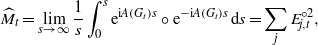
where Er is the rth idempotent of the spectral decomposition of A(Gt) = ∑jλjEj. In other words, Ej,t represents the orthogonal projection onto the eigenspace ker(A(Gt) − λjI), where λj is the jth eigenvalue of A(Gt). The ijth entry of  is the average probability that a walker is found at node vj (starting at node vi). Remarkably,
  is rational [38].
In our model of growth based on CTQWs, the attaching probability is defined by ![$\mathbb{P}[\{ {v}_{t+1},{v}_{j}\} \in E\left ({G}_{t+1}\right )]=[{\widehat{M}}_{t}]_{i,j}$](https://content.cld.iop.org/journals/1742-5468/2013/08/P08016/revision1/jstat482661ieqn170.gif) , if we assume that the walker started from node vi at the tth iteration of the growth process. Depending on the starting node vi, we get a different attaching probability, which will be completely defined by Gt. The time length of the walk is not relevant given that
, if we assume that the walker started from node vi at the tth iteration of the growth process. Depending on the starting node vi, we get a different attaching probability, which will be completely defined by Gt. The time length of the walk is not relevant given that  is defined as a limit for s → ∞.
Algorithm. Let Kn denote the complete graph on n vertices. This is the unique graph with n(n − 1)/2 edges. Let [A]i be the ith row of a matrix A. The growth of a graph based on CTQWs starts with Gm = Km. Then, for every t > m, we sample m neighbours vj1,vj2,...,vjm of the new node vt from the distribution ![$[{\widehat{M}}_{t-1}]_{i}$](https://content.cld.iop.org/journals/1742-5468/2013/08/P08016/revision1/jstat482661ieqn188.gif) and create m edges {vt,vj1},{vt,vj2},...,{vt,vjm}.
and create m edges {vt,vj1},{vt,vj2},...,{vt,vjm}.
The edges are all added at the same time, after m distinct CTQWs have been performed on Gt−1. The starting node vi of the CTQW can be arbitrarily chosen. In the main body of the paper we report the results obtained for three different choices of the starting node, namely: (a) the first node, (b) the last node added to the graph and (c) a different randomly sampled node for each step of the algorithm. The initial condition Gm = Km can be also relaxed.
This simple growth algorithm, based on the sampling of new edges according to the time-average of the attaching probability distribution, suffers from the fact that the evaluation of the Cesaro mean requires the full spectrum of the adjacency matrix A(Gt). This is the critical step. In fact, although efficient schemes exist to compute the few largest eigenvalues of a symmetric matrix of size n, the time complexity of the computation of the whole spectrum is ∼O(n3). At a first analysis, it follows that the number of steps needed to sample a graph of t nodes constructed with our method is of the order O(t3). Sampling a CTQW-based graph is much more costly than sampling a BA random graph, for which the most efficient algorithm runs in O(t).
A.2. Network metrics
Let G = (V,E) be a graph on n nodes {v1,v2,...,vn}. The average degree of G is  . Let d(vi) = k, for a given node vi∈V(G); then the average degree of the neighbours of vi is denoted by
  . We say that two nodes vi,vj∈V(G) are connected if there is l∈Z+ such that [Al(G)]i,j > 0. Equivalently, vi and vj are connected if there is a walk from vi to vj. A walk from vi to vj is a sequence of edges {{vi = i0,i1},{i1,i2},...,{in−1,in = vj}}, where the nodes are not necessarily all distinct. When the nodes of a walk are all distinct then we call it a path. The length of a path is the number of edges in the path. The distance d(i,j) between vi,vj∈V(G) is defined as the length of the path from vi to vj with the minimum number of edges. The average shortest path length of G is then defined as ℓ:=1/(n(n − 1))∑i,jd(i,j). If there is no path containing vi and vj then d(i,j) = ∞, by convention. Consequently, ℓ is finite only for connected graphs, i.e. when every pair of nodes of the graph is connected by a path. The graphs generated by the algorithm are connected by construction. The clustering coefficient Ci of a node vi∈V(G) is a measure of the local cohesion at vi. Taking k = d(vi), we have Ci:=1/(k(k − 1))T(vi), where T(vi) is the number of different triangles containing vi. A triangle is a graph of the form ({vi,vj,vk},{{vi,vj},{vj,vk},{vi,vk}}). The clustering coefficient of G is the average of the clustering coefficients of all nodes:
  . (See [49] for a general reference on these notions.)
Real networks usually exhibit degree–degree correlations. For instance, in some networks (mostly social, information and communication networks) high-degree nodes are preferentially linked to other high-degree nodes, while in biological and technological networks high-degree nodes are preferentially linked to low-degree nodes [1]. The existence of degree–degree correlations can be quantified in different ways. One of the most common methods is by computing  as a function of k. If a graph is uncorrelated then the degree of the neighbours of a node of degree k does not depend on k, and it is possible to show that
  . In real networks we observe that
  depends on k: if
  increases with k, we say that the network has assortative degree–degree correlations; on the contrary, if
  decreases when k increases, we say that the network has disassortative degree–degree correlations. (See [50] for an in-depth discussion about degree correlations in networks.) In most real networks,
  (with a little abuse of notation) and the exponent ν can be effectively used to quantify degree–degree correlations: ν > 0 and ν < 0 define assortative and disassortative networks, respectively [51]. The larger the modulus of ν, the stronger are the degree–degree correlations.