

Abstract
We present a complementary estimation of the critical exponent  of the specific heat of the 5D random-field Ising model from zero-temperature numerical simulations. Our result
  is consistent with the estimation coming from the modified hyperscaling relation and provides additional evidence in favor of the recently proposed restoration of dimensional reduction in the random-field Ising model at D = 5.
Export citation and abstract BibTeX RIS
The random-field Ising model (RFIM) is one of the archetypal disordered systems [1–15], extensively studied due to its theoretical interest, as well as its close connection with experiments in condensed-matter physics [15–19]. Its beauty stems from the combination of random fields and the standard Ising model that creates rich and complicated physical phenomena, responsible for a great volume of research over the last 40 years and more. It is well established that the physically relevant dimensions of the RFIM lay between 2 < D < 6, where  and
and  are the lower and upper critical dimensions of the model, respectively. For
  one expects the standard mean-field (MF) behavior [1, 8–10, 20, 21], whereas exactly at
  the notoriously obscuring logarithmic corrections appear [22].
In the last few years, the development of a powerful panoply of simulation and statistical analysis methods [23] have set the basis for a fresh revision of the problem. In fact, some of the main controversies have been resolved, the most notable being the illustration of critical universality in terms of different random-field distributions [24–26] and the restoration of supersymmetry and dimensional reduction at D = 5 [27–29] (see also [30–33] for additional evidence in this respect).
In particular, the large-scale numerical simulations of the 5D RFIM reported in [27] have provided high-accuracy estimates for the spectrum of critical exponents and for several universal ratios (see table III in [27]), with one missing element: that of the direct computation of the critical exponent  of the specific heat. Let us point out that the specific heat of the RFIM is of experimental interest [18] and that the value of
  has severe implications for the validity of the fundamental scaling relations, and in particular for the Rushbrooke relation,
  , that has been the most controversial of all [34–38]. Therefore a strong command on this aspect of the model's critical behavior is necessary. In the current work we fill this gap by performing additional simulations and scaling analysis that allow us to directly compute
  for the 5D RFIM and to therefore present a complete picture of the scaling behavior of the specific heat. Our final estimate,
  , agrees well with that of the 3D Ising universality class,
  [39], and therefore constitutes additional evidence in favor of our recently proposed restoration of dimensional reduction at D = 5 [27–29].
The RFIM Hamiltonian is

with the spins  occupying the nodes of a hyper-cubic lattice in space dimension D with nearest-neighbor ferromagnetic interactions J and hx independent random magnetic fields with zero mean and dispersion
  . Here we consider the Hamiltonian (1) on a D = 5 hyper-cubic lattice with periodic boundary conditions and energy units J = 1. Our random fields hx follow either a Gaussian
  , or a Poissonian
  distribution of the form

where  and
and  the disorder-strength control parameter.
As it is well-established, in order to describe the critical behavior of the model one needs two correlation functions, namely the connected and disconnected propagators,  and
and  :
:

where the  are thermal mean values as computed for a given realization, a sample, of the random fields {hx}. Over-line refers to the average over the samples. Following the prescription of [23], for each of these two propagators we scrutinize the second-moment correlation lengths, denoted as
  and
and  , respectively.
Our numerical simulations for the 5D RFIM are described in [27]. We therefore outline here the very necessary details. We simulated lattice sizes from  to
to  . For each pair of (L,
  ) values we generated ground states for 107 samples—for the additional simulations at the most accurate determinations of the critical points shown below in figures 4 and 5, 106 samples were generated—exceeding previous relevant studies [22] by a factor of 103 on average. The calculation of the ground states of the RFIM was based on the well-established mapping [34–38, 40–55] to the maximum-flow problem [56–58]. We used our own C version of the push-relabel algorithm of Tarjan and Goldberg [59], involving some technical modifications proposed by Middelton and collaborators for further efficiency [46, 47]. Suitable generalized fluctuation-dissipation formulas and reweighting extrapolations have facilitated our analysis, as exemplified in [23]. A comparative illustration in favor of the numerical accuracy of our scheme is shown in figure 1 for the universal ratio
  of an L = 10 Gaussian RFIM and four different simulation sets, as outlined in the panel.

Figure 1. Connected correlation length in units of the system size L versus  for the 5D Gaussian RFIM and a system of linear size L = 10. Four distinct simulation sets are shown, corresponding to different simulation values,
  , and different sets of random-field realizations. The inset illustrates the reweighting error-evolution for the fourth simulation set with
  and
and  .
.
Download figure:
Standard image High-resolution imageThe specific heat of the RFIM can be estimated using ground-state calculations in two complementary frameworks, both based on the analysis of singularities of the bond-energy density EJ [60]. This bond-energy density is the first derivative  of the ground-state energy with respect to the random-field strength
  [34, 35]. The derivative of the sample averaged quantity
  with respect to
  then gives the second derivative with respect to
  of the total energy and thus the sample-averaged specific heat C. The singularities in C can also be studied by computing the singular part of
  , as
, as  is just the integral of C with respect to
  . Thus, one may estimate
  by studying the behavior of
  at
at  [34], via the scaling form

where  , b, and
  are non-universal constants, and
  is the universal corrections-to-scaling exponent.
Of course, the use of equation (4) for the application of standard finite-size scaling methods requires an a priori knowledge of the exact value of the critical random-field strength  (see also the analysis below in figures 4 and 5). Although we currently have at hand such high-accuracy estimates of the critical fields for both types of the random-field distributions under study [27], we start our analysis with an alternative to this approach. In particular, we implement a three lattice-size variant of the original quotients method8, also known as phenomenological renormalization [61–63] that has been described in detail in [26] and already successfully applied to the D = 3 [23] and D = 4 [25] models. The main idea in this perspective, given that
  , is the elimination of the non-divergent background term
  in equation (4) by considering three lattice sizes in the following sequence:
  (see figure 2 for an instructive illustration of the three-lattice variant of the quotients method based on the crossings of
  ). Taking the quotient of the differences at the crossings of the pairs
  and
and 

one obtains the following scaling formula for the bond-energy density [26]

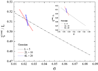
Figure 2. Connected correlation length in units of the system size L versus  for the 5D Gaussian (main panel) and Poissonian (inset) RFIM. An illustrative example of the three lattice-size sequence
  used in the application of the modified quotients method is shown (see equations (5) and (6)). Data taken from [27].
Download figure:
Standard image High-resolution imageOur results for the effective exponent ratio  as a function of
  —where
  is set to the 3D Ising value
  [39]—are shown in figure 3. The dashed line marks the estimate
  of the 3D Ising universality class, where we have used the values
  and
and  [39]. A few comments are in order: (i) Clearly, there exist large corrections to scaling for the sequence of smaller sizes
  and
and  that obscure the application of any finite-size scaling approach. (ii) The remaining data points (
 ,
,  , and
, and  ) do not allow for a safe extrapolation of the ratio
  to
to  , although the general trend of the data appears to be on the right track and, in fact, joint polynomial fits with a shared constant term do approach the value
  but with a rather bad fitting quality. (iii) Larger system sizes would be needed to clarify this point, but are unfortunately out of reach with our current resources.
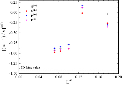
Figure 3. Effective exponent ratio  versus
  for all random-field distributions and crossing points considered in this work. Note the notation
  , where Z stands for the distribution—G for Gaussian and P for Poissonian—and the superscript x for the connected (con) or disconnected (dis) type of the universal ratio
  , used for the application of the quotients method (see equations (5) and (6)).
Download figure:
Standard image High-resolution imageGuided by these qualitative results of the phenomenological-renormalization approach, we have performed, at a second stage, additional simulations at the critical points  and
and  of the Gaussian and Poissonian models, respectively [27]. In figures 4 and 5 we report on the finite-size scaling behavior of the bond-energy density at these critical points for the whole spectrum of system sizes studied, alongside with the resulting estimates for the ratio
  . In both panels the solid lines are fits of the form (4), where the different colors correspond to different fixed values of
  . Black curves correspond to the value
  of the 3D Ising universality class [39], whereas red curves to the value 0.66 estimated in [27]. The fitting quality, measured in terms of
  /dof, where dof measures the number of degrees of freedom, and the minimum system size,
  , used in the fits are as follows:
  ,
,  for the Gaussian model (figure 4) and
  ,
,  for the Poissonian model (figure 5). Note that there was practically no variation in the fitting quality moving from
  down to 0.669. Using now the estimate
  for the critical exponent of the correlation length, simple algebra and error propagation produces values for
  within the range 0.10–0.13. Taking an average over the values of
  obtained from the black curves with
  , we give our final estimate for the critical exponent
  to be
to be

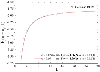
Figure 4. Finite-size scaling behavior of the bond-energy density at the critical random-field strength  of the 5D Gaussian RFIM. The lines are fittings of the form (4) with different
  values, as indicated in the panel.
Download figure:
Standard image High-resolution image
Figure 5. Finite-size scaling behavior of the bond-energy density at the critical random-field strength  of the 5D Poissonian RFIM. The lines are fittings of the form (4) with different
  values, as indicated in the panel.
Download figure:
Standard image High-resolution imageThis is compatible to the value  obtained in [27] via the modified hyperscaling relation
  , where
  and
and  are the corresponding anomalous dimensions of the connected and disconnected correlation functions (see equation (3)) and also agrees nicely with the 3D Ising universality benchmark
  [39].
[39].
As an additional consistency check of our results shown in figures 4 and 5, we depict in figure 6 the scaling behavior of the specific heat C, obtained from the derivative of the bond-energy density with respect to the random-field strength  , at the critical point. Note that the horizontal axis has been rescaled to
  (remember that as in the standard case
  ), and
  has been set to the value
  via
via  and
and  of the 3D Ising universality class [39]. As expected the data become rather noisy with increasing system size, forcing us to exclude from our fittings the larger system sizes L = 20 and L = 24, where statistical errors are larger than 30%. Although we illustrate for the benefit of the reader data for the complete spectrum of system sizes studied, the solid lines are simple linear fits within the range L = 4–16 with a very good fitting quality indeed:
  and 2.03/6 for the Gaussian and Poissonian models, respectively.
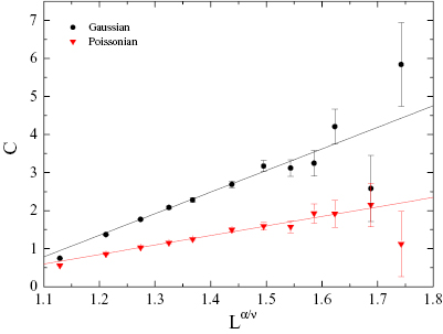
Figure 6. Scaling behavior of the specific heat C for both models considered in this work, as indicated in the panel. For a detailed discussion on the scaling laws and the fitting tests refer to the main text.
Download figure:
Standard image High-resolution imageTo summarize, using extensive numerical simulations at zero temperature we provided a high-precision estimate of the specific-heat's critical exponent of the 5D RFIM. Our final result  is fully consistent with the estimation coming from the modified hyperscaling relation given in [27], and also supports the recent results of [29] for the restoration of supersymmetry and dimensional reduction in the RFIM at D = 5. We close this contribution with figure 7 and an overview of the critical exponent
  of the RFIM at all physically relevant dimensions. Two sets of data points are shown, as outlined in the caption, corroborated by a graphical validation of the Rushbrooke relation in the corresponding inset. Whilst the collative results of figure 7 are reassuring and settle down previous controversies in the random-field problem originating from defective estimations of the critical exponent
  , for reasons of clarity we sould like to point out that the large error at D = 3 stems from the joint fits of
 ![$[(\alpha - 1)/\nu]^{\rm (ef\,\!f)}$](https://content.cld.iop.org/journals/1742-5468/2019/9/093203/revision1/jstatab3987ieqn122.gif) performed over several random-field distributions (including the double Gaussian distribution) and the large scaling corrections via
performed over several random-field distributions (including the double Gaussian distribution) and the large scaling corrections via  [23, 24]—for further details and graphical explanations on this aspect we refer the interested reader to figures 6 and 7 of [23].
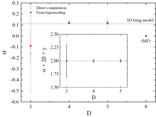
Figure 7. Critical exponent  of the specific heat of the RFIM as a function of the spatial dimension D. Two sets of data points are shown: estimates from direct computation (open squares) and from the modified hyperscaling relation (filled circles) via previously obtained results for the exponents
  ,
,  , and
, and  . The dashed line marks the 3D Ising value
  [39]. The filled star signals the MF value
  , expected to hold at
  . Inset: verification of the Rushbrooke scaling relation. For the estimation of the magnetic critical exponents
  and
and  we have used the standard relations
  and
and  . The dashed line is located exactly at the value 2. Data taken from this work and from [23–27].
Download figure:
Standard image High-resolution imageAcknowledgments
We acknowledge partial financial support from Ministerio de Economía, Industria y Competitividad (MINECO, Spain) through Grants No. FIS2015-65078-C2 and PGC2018-094684-B-C21, and from the European Research Council (ERC) under the European Union's Horizon 2020 research and innovation program (Grant No. 694925).
Footnotes
- 8
The general approach in the quotients method is to compare observables computed in pair of lattices
 . We start imposing scale-invariance by seeking the L-dependent critical point: the value of such that , i.e. the crossing point for (see also figure 2 for the case where ). For dimensionful quantities O, scaling in the thermodynamic limit as , we consider the quotient at the crossing. Thus, we have , where , and the scaling-corrections exponent are universal.
 - 9
See also the relevant statistical tests with respect to the value of
for the other thermodynamic observables in [27].


