

Abstract
Land use change in South America, mainly deforestation, is a large source of anthropogenic CO2 emissions. Identifying and addressing the causes or drivers of anthropogenic forest change is considered crucial for global climate change mitigation. Few countries however, monitor deforestation drivers in a systematic manner. National-level quantitative spatially explicit information on drivers is often lacking. This study quantifies proximate drivers of deforestation and related carbon losses in South America based on remote sensing time series in a systematic, spatially explicit manner. Deforestation areas were derived from the 2010 global remote sensing survey of the Food and Agricultural Organisation Forest Resource Assessment. To assess proximate drivers, land use following deforestation was assigned by visual interpretation of high-resolution satellite imagery. To estimate gross carbon losses from deforestation, default Tier 1 biomass levels per country and eco-zone were used. Pasture was the dominant driver of forest area (71.2%) and related carbon loss (71.6%) in South America, followed by commercial cropland (14% and 12.1% respectively). Hotspots of deforestation due to pasture occurred in Northern Argentina, Western Paraguay, and along the arc of deforestation in Brazil where they gradually moved into higher biomass forests causing additional carbon losses. Deforestation driven by commercial cropland increased in time, with hotspots occurring in Brazil (Mato Grosso State), Northern Argentina, Eastern Paraguay and Central Bolivia. Infrastructure, such as urban expansion and roads, contributed little as proximate drivers of forest area loss (1.7%). Our findings contribute to the understanding of drivers of deforestation and related carbon losses in South America, and are comparable at the national, regional and continental level. In addition, they support the development of national REDD+ interventions and forest monitoring systems, and provide valuable input for statistical analysis and modelling of underlying drivers of deforestation.
Export citation and abstract BibTeX RIS

Content from this work may be used under the terms of the Creative Commons Attribution 3.0 licence. Any further distribution of this work must maintain attribution to the author(s) and the title of the work, journal citation and DOI.
1. Introduction
Land use change, mainly deforestation, is the second largest source of anthropogenic CO2 emissions, and causes a net reduction of carbon storage in terrestrial ecosystems as well as other environmental impacts such as biodiversity loss (IPCC 2013). The vast majority of land use change occurs in tropical regions, with Central and South America having the highest net emissions from land use change from the 1980s to 2000s (IPCC 2013). Reducing emissions from deforestation and forest degradation, and enhancing carbon stocks (REDD+) in (sub−) tropical countries is thus a necessary component of global climate change mitigation. Within the REDD+ framework, participating countries are given incentives to develop national strategies and implementation plans that reduce emissions and enhance sinks from forests and to invest in low carbon development pathways. Identifying and addressing the causes or drivers of anthropogenic forest change is considered crucial within the REDD+ framework (UNFCCC 2014), and should be incorporated in national forest monitoring systems.
Few countries, however, monitor deforestation drivers in a systematic manner and national-level quantitative spatially explicit information on drivers is often lacking (De Sy et al 2012, Hosonuma et al 2012). The distinction between proximate and underlying drivers is important for assessment purposes. Proximate or direct drivers of deforestation are human activities that directly affect the loss of forests (Geist and Lambin 2001), and can be assessed by linking forest area change to specific human activities and follow-up land use (De Sy et al 2012). Remote sensing can provide essential information on the intensity, type and pattern of deforestation, and on the follow-up land use in order to attribute deforestation to specific human activities (Gibbs et al 2010, De Sy et al 2012, GOFC-GOLD 2014). Statistical analysis and modelling of this information, in turn, can be useful for the assessment of underlying drivers (Kissinger et al 2012) which are complex interactions of social, political, economic, technological and cultural forces (Geist and Lambin 2001).
Forest loss and related carbon losses in South America have been extensively studied from the continental to the (sub)national scale (DeFries et al 2002, Baccini et al 2012, Eva et al 2012, Harris et al 2012, Hansen et al 2013, Achard et al 2014, Beuchle et al 2015, Velasco Gomez et al 2015) but the link to specific proximate drivers is not made. Clark et al (2012) and Graesser et al (2015) studied land use change across the South American continent in a systematic manner with MODIS imagery which gives some insight into drivers of deforestation. MODIS imagery, however, cannot accurately detect small-scale agricultural clearings (<25 ha) and infrastructure expansion due to its low spatial resolution (GOFC-GOLD 2014). Other research that links forest loss or forest carbon emissions to drivers used aggregated continental scale (Geist and Lambin 2002, Hosonuma et al 2012, Houghton 2012) or local scale data (Morton et al 2006, Barona et al 2010, Clark et al 2010, Müller et al 2012, 2014, Gibbs et al 2015). Several studies link overall deforestation rates directly to underlying drivers (DeFries et al 2010, Malingreau et al 2012). Linking driver-specific deforestation rates (e.g. agricultural expansion) to relevant underlying drivers (e.g. agricultural commodity prices) can provide more insight into complex deforestation pathways.
Although it is clear that agricultural expansion is the main driver of deforestation in South America (Geist and Lambin 2002, Gibbs et al 2010, Hosonuma et al 2012, Houghton 2012), less is known about the magnitude and the spatial and temporal distribution of different types of agricultural and non-agricultural drivers contributing to forest loss and related carbon emissions. Gaining insight in spatiotemporal dynamics is essential since drivers of forest loss vary from region to region and change over time (Rudel et al 2009, Boucher et al 2011).
Accordingly, our research aims to quantify proximate drivers of deforestation, their spatiotemporal dynamics and related carbon losses in South America at continental and national scales using a comprehensive, systematic remote sensing analysis. This new dataset will provide insight into complex deforestation pathways and be a valuable source of information for international climate change mitigation and REDD+ monitoring strategies.
2. Data and methods
The 2010 global Remote Sensing Survey of the United Nations Food and Agricultural Organisation (FAO) Forest Resource Assessment was used as input to determine deforestation areas (section 2.1). To assess proximate drivers, land use following deforestation was assigned by visual interpretation of high-resolution satellite imagery (section 2.2). To estimate gross carbon losses from deforestation, default Tier 1 biomass levels per country and eco-zone were used (section 2.3).
2.1. Forest area loss
In a coordinated effort, the European Joint Research Centre (JRC) and the FAO produced estimates of forest land use change from 1990 to 2005 for the Remote Sensing Survey of the Global Forest Resources Assessment 2010 of FAO (FAO FRA-2010 RSS) (FAO & JRC 2012). These estimates were based on a systematic sampling design with sample units of 10 × 10 km centred on each degree latitude–longitude confluence point (Eva et al 2012, FAO & JRC 2012, Achard et al 2014).
Unfortunately the FAO FRA-2010 RSS currently only covers a limited time period from 1990 to 2005. As mentioned in the introduction, other deforestation datasets are available (e.g. Hansen et al 2013) that provide wall-to-wall data extending to 2010 or even later. The FAO FRA-2010 RSS, however, employs a land use classification that is better suited for assessing drivers than a land cover classification. In addition, the FAO FRA-2010 RSS is a global study with consistent methods and time series that could be extended to include more recent periods. Despite the time period limitation, and in view of the paucity of quantitative data on deforestation drivers and related carbon losses, this study provides an unique and relevant overview of the drivers of deforestation in South America, as well as showing that this is achievable with a sample-based time series approach.
We briefly describe the methodology of the FAO FRA-2010 RSS dataset (FAO & JRC 2012), because it served as input data for our study. Medium resolution satellite imagery (mainly Landsat) was acquired for each sample unit, as close as possible to reference years 1990, 2000 and 2005. After pre-processing, the satellite imagery was used in an automated multi-date image segmentation to subdivide the sample unit (10 000 ha) into delineated areas (polygons) with similar spectral and structural attributes. The target minimum mapping unit was 5 ha. On the segmented imagery, a supervised automated land cover classification was carried out, which later was converted to a land use classification with the help of expert human interpretation. The main land use classes were Forest, Other wooded land, and Other land, which are based on FAO forest definitions (FAO 2010). Areas lacking data due to clouds, poor satellite coverage or low quality imagery in any of the reference years were considered an unbiased loss of information and were not analysed. This sample grid provided 1542 sample units in South America, of which 1392 sample units had data for all years and were consequently processed (figure 1).
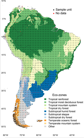
Figure 1. Location of sample units (FAO & JRC 2012), and FAO ecological zones (FAO 2001) in South America.
Download figure:
Standard image High-resolution image2.2. Follow-up land use
Land use following a deforestation event was assigned a more detailed land use class, i.e. follow-up land use class, as a proxy for the proximate cause of change. Assessing land use is more challenging than assessing land cover, as factors other than spectral reflectance are important. So, expert human interpretation and relatively fine-scale satellite imagery are required to interpret the proximate causes of deforestation. To assign follow-up land use in this study, we used parameters such as land cover, the presence of certain features within or near changed areas (e.g. crop rows, watering holes, fences) and to a limited extent the spatial context and location of change (e.g. distance to settlements, concessions).
Table 1 gives an overview of the follow-up land use classes and their descriptions, that we used as proxies for the proximate deforestation driver. These land use classes are based on the proximate deforestation drivers as described in Hosonuma et al (2012) i.e. agricultural expansion, mining, infrastructural and urban expansion. The class 'other land use' was added for deforested areas where no clear human activity could be distinguished. The 'other land use' subclasses are chosen in such a way that our classification could be translated to IPCC land categories (e.g. wetlands, grasslands) (IPCC 2013) and FAO land use definitions (e.g. other wooded land) (FAO 2010). The water class was added to account for forest loss due to inundation by lakes, meandering rivers and dam reservoirs.
Table 1. Follow-up land use classes and their description.
| Follow-up land use | Description | |
|---|---|---|
| Mixed agriculture | Mix of agricultural land uses | |
| Commercial crop | Land under cultivation for crops, characterised by medium (2–20 ha) to large (>20 ha) field sizes | |
| Agriculture | Smallholder crop | Land under cultivation for crops, characterised by very small (<0.5 ha) to small field sizes (0.5–2 ha) |
| Tree crops | Miscellaneous tree crops (e.g. coffee, palm trees), orchards and groves | |
| Pasture | Land used predominantly for grazing; in either managed/cultivated (pastures) or natural (grazing land) setting; includes grazed woodlands | |
| Urban and Settlements | Urban, settlements and other residential areas | |
| Infrastructure | Roads and built-up | Roads, built-up areas and other transport, industrial and commercial infrastructures |
| Mining | Land used for extractive subsurface and surface mining activities (e.g. underground and strip mines, quarries and gravel pits), including all associated surface infrastructure | |
| Other land use (general) | All land that is not classified as forest, agriculture, infrastructure, mining and water | |
| Bare land | Barren land (exposed soil, sand, or rocks) | |
| Other land use | Other wooded land | Land not classified as forest, spanning more than 0.5 ha; with trees higher than 5 m and canopy cover of 5%–10%, or trees able to reach these thresholds in situ, or with a combined cover of shrubs, bushes and trees above 10%. It does not include land that is predominantly under agricultural or urban land use (FAO 2010) |
| Grass and herbaceous | Land covered with (natural) herbaceous vegetation or grasses | |
| Wetlands | Areas of natural vegetation growing in shallow water or seasonally flooded environments. This category includes Marshes, swamps, and bogs | |
| Water | Natural (river, lake etc) or man-made waterbodies (e.g. reservoirs) | |
| Unknown land use | All land that cannot be classified (e.g. due to low resolution imagery) | |
We have used several key criteria to classify land uses. Cropland can be detected by plough lines, rectilinear shapes, and nearby roads and infrastructure (Clark et al 2010). We used field size as a proxy for agricultural development and mechanisation (Kuemmerle et al 2013, Fritz et al 2015). We classified cropland with very small to small fields (<2 ha) as smallholder cropland, and cropland with medium to large fields (>2 ha) as commercial cropland (>2 ha). Tree crops can be recognised by perennial vegetation and the regular spacing of the tree plants (Clark et al 2010). Pasture can be distinguished by trails and watering holes, and is usually more heterogeneous in colour and texture than cropland (Clark et al 2010).
In order to achieve a detailed follow-up land use classification, we performed the following steps:
- (1).We selected those polygons of each sample unit within the FAO FRA-2010 RSS dataset that were deforested, either in the interval between 1990 and 2000 or 2000 and 2005 according to the FAO FRA-2010 RSS classification, i.e. changed from Forest to Other wooded land or to Other land.
- (2).Each of these deforested polygons was assigned a single follow-up land use class (table 1) by means of visual interpretation by an expert. If more than one land use was present, the most dominant one in terms of area or human activity (e.g. a road with shrubs on the side is assigned road) was chosen. For the visual interpretation a variety of satellite imagery was used such as Landsat, Google Earth imagery (Google Earth 2015) and ESRI world imagery basemaps. For the Brazilian Amazon, Terraclass 2008 data (Coutinho et al 2013) was used to help with the interpretation. We used satellite imagery acquired as close as possible to the deforestation period (e.g. 2000 or 2005).
- (3).In addition to follow-up land use, the source and year of the satellite imagery used for the interpretation (e.g. Google Earth 2009) and the confidence (low—medium—high) in the interpretation was documented.
- (4).For the areas with low confidence, e.g. due to low resolution imagery, land use and remote sensing experts with local knowledge were consulted. These experts were provided with the follow-up land use classification and descriptions in order to classify the areas based on their local knowledge, and additional sources available to them such as high resolution satellite imagery and land use maps.
- (5).Finally, all areas were double checked, and if necessary corrected for errors and consistency. This means each forest loss area has been looked at least twice by one or more experts.
In the end, 77.8% of follow-up land use classification was assigned with high confidence, 17.6% with medium confidence and only 4.6% with low confidence. In general, small-scale land uses, such as smallholder cropland, were classified with less confidence due to their smaller scale and because these land uses occur more in locations with higher cloud cover and with lower availability of high resolution imagery (Andean countries, Amazon rainforest). In addition, the class 'other land use' also had a higher portion of low confidence classification since it is not always possible to assess whether these areas are used for agriculture. For all land uses, the confidence level was also influenced by the date of the available imagery.
2.3. Carbon losses
Gross carbon loss per sample unit was calculated using spatially explicit forest biomass information. A recent study by Langner et al (2014) combined a global forest mask derived from the Globcover-2009 map (Bontemps et al 2011), FAO ecological zones (eco-zones; FAO 2001) and the pan-tropical above ground biomass (AGB) datasets of Saatchi (Saatchi et al 2011) and Baccini (Baccini et al 2012) to derive mean AGB levels in forests (for intact, non-intact and overall forest) per eco-zone and country as an alternative to IPCC Tier 1 values.
We used the country eco-zone AGB forest values derived from the combined Saatchi and Baccini AGB maps (table 3 in supplementary information of Langner et al 2014). We used AGB values for the overall forest category since we did not have information on whether the deforested area had intact or non-intact forest. For those AGB forest values where the number of samples per eco-zone was too small, we used the combined AGB values of that eco-zone at the continental (South America) or tropical scale. If these AGB values were also not present we used IPCC Tier 1 AGB values for America (IPCC 2006). For Argentina and Chile, which were not included in Langner et al (2014), we used the same procedure. Table 2 provides an overview of the AGB values per country eco-zone used in our study.
Table 2. AGB mean forest values (t ha−1) per eco-zone and country based on combined Saatchi and Baccini datasets (unless otherwise indicated); Source: Langner et al (2014), table 3 in their supplementary information.
| Eco-zone | Argentina | Bolivia | Brazil | Chile | Colombia | Ecuador | French Guiana | Guyana | Paraguay | Peru | Suriname | Uruguay | Venezuela |
|---|---|---|---|---|---|---|---|---|---|---|---|---|---|
| Tropical rainforest | — | 211 | 239 | — | 237 | 237 | 280 | 269 | 79 | 276 | 273 | — | 250 |
| Tropical moist deciduous forest | 123a | 180 | 98 | — | 88 | 123a | — | 222 | 80 | — | 252 | — | 154 |
| Tropical dry forest | 79a | 95 | 68 | — | 105 | 116 | — | — | 68 | 79a | — | — | 106 |
| Tropical mountain system | 195a | 199 | 126 | — | 162 | 187 | — | 280 | — | 208 | — | — | 240 |
| Subtropical humid forest | 110a | — | 110 | — | — | — | — | — | — | — | — | 110a | — |
| Subtropical dry forest | — | — | — | 57b | — | — | — | — | — | — | — | — | — |
| Subtropical steppe | 80c | — | — | — | — | — | — | — | — | — | — | — | — |
| Temperate mountain system | 130c | — | — | — | — | — | — | — | — | — | — | — | — |
| Temperate oceanic forest | — | — | — | 180c | — | — | — | — | — | — | — | — | — |
aContinental (America) value (Langner et al 2014, table 2a in their supplementary information). bGlobal value (Langner et al 2014, table 1 in their supplementary information). cIPCC continental (America) value. — Eco-zone and country combinations that do not exist or are without forest loss.
We derived total biomass from AGB by applying the equation (1) used by Saatchi et al (2011):

Total carbon was considered to be 50% of total biomass as in Achard et al (2014). We considered only the maximum potential loss of carbon stock from deforestation, assuming a carbon stock of zero in potential follow-up land uses, that could be emitted to the atmosphere over a long time period. We did not account for soil carbon loss.
2.4. Aggregation to regional scale
Deforestation and related carbon losses per driver were scaled up from the sample to the continental and national scales using a statistical extrapolation similar to FRA-2010 RSS (FAO & JRC 2012). Cloudy areas were considered an unbiased loss of data, with the assumption that cloudy areas had the same proportion of land uses as cloud-free areas within a single sample unit. This was accomplished by considering the ratio of forest area or carbon loss per driver proportional to the 'visible land' area of the sample unit. The 'visible land' area was the full sample unit area (100 km2) minus cloudy and 'permanent water' areas (i.e. sea or inland water in all considered years).
Estimates of forest area and carbon losses per driver for each sample unit for the two periods (1990–2000 and 2000–2005) were annualised based on the acquisition dates of the imagery for that sample unit, with the assumption that the change rates were constant during the two time intervals. The average time length across all sample units was 11.9 years for the 1990–2000 epoch and 4.9 years for the 2000–2005 epoch.
Each sample unit was assigned a weight (wi) (2), equal to the cosine of its latitude (coslati), because the actual area represented by a sample unit decreased with latitude due to the curvature of Earth:

The proportions of forest area changes and carbon losses per driver were extrapolated to a given region (the full continent or one specific country) using the Horvitz–Thompson direct estimator (Särndal et al 1992) (3)

where

and where xic is the proportion of forest cover change or carbon loss in the ith sample unit and wi is the weight of the ith sample unit. The total area of change or total loss of carbon for this region (Driverregion) is then obtained from:

where A is the total area of the region (excluding permanent water).
We used the usual variance estimation of the mean for this systematic sampling as follows:

The standard error (SE) is then calculated as:

The SE represents only the sampling error. Countries or states with a SE of more than 35% for forest area and carbon losses estimates were not reported at the national scale (i.e. French Guyana, Guyana, Ecuador and Chile).
3. Results
3.1. Deforestation and carbon losses per driver from 1990 to 2005
We estimated that total deforested area and related gross carbon losses in South America from 1990 to 2005 reached 57.7 million ha and 6 460 Tg C, respectively (table 3). Agriculture was the dominant follow-up land use (88.5%), in particular pasture (71.2%) and to a lesser extent commercial cropland (14.0%). In the non-agricultural category, other land use was the largest driver (6.5%). This class can be further subdivided in other wooded land (4.4%), wetlands (1.4%), grass and herbaceous (0.6%) and bare land (0.1%). The contribution of smallholder cropland (2.0%), infrastructure (1.7%) and water (3.0%) was small. Within the infrastructure class, urban and settlements accounted for 0.9%, roads and built-up areas for 0.6% and mining for 0.2% of deforestation. The water driver can be divided into natural (1.3%) and man-made water bodies (1.8%). Unknown land use only represented a small fraction (0.2%) of total deforestation.
Table 3. Estimates of deforested area (103 ha (SE) and per cent of total) and related carbon loss (Tg C (SE) and per cent of total) per follow-up land use from 1990 to 2005.
| Area | Carbon loss | |||
|---|---|---|---|---|
| Follow-up land use | 103 ha (SE) | % | Tg C (SE) | % |
| Mixed agriculture | 470 (233) | 0.8 | 57 (32) | 0.9 |
| Smallholder crop | 1 168 (272) | 2.0 | 173 (42) | 2.7 |
| Commercial crop | 8 100 (1463) | 14.0 | 782 (162) | 12.1 |
| Tree crops | 243 (75) | 0.4 | 20 (6) | 0.3 |
| Pasture | 41 118 (3244) | 71.2 | 4 624 (431) | 71.6 |
| Agriculture total | 51 099 (3618) | 88.5 | 5 657 (472) | 87.6 |
| Infrastructure | 985 (346) | 1.7 | 124 (52) | 1.9 |
| Other land use | 3 770 (517) | 6.5 | 433 (65) | 6.7 |
| Water | 1 748 (543) | 3.0 | 228 (79) | 3.5 |
| Unknown land use | 131 (108) | 0.2 | 18 (15) | 0.3 |
| Other total | 6 634 (897) | 11.5 | 802 (123) | 12.4 |
| Total | 57 733 (3837) | 100 | 6 460 (501) | 100 |
The spatially explicit nature of our dataset shows the distribution of follow-up land use across the continent (figure 2(a)). The Brazilian arc of deforestation was dominated by pasture expansion, except for a commercial crop agriculture cluster in Mato Grosso State. Considerable deforestation, mainly due to the expansion of pasture, occurred in the Brazilian Pantanal and Cerrado ecoregions. Toward the Atlantic coast, in the Mata Atlântica ecoregion, the follow-up land use became more diverse with a mix of pasture, commercial cropland and tree crops. Pasture expansion was also an important driver of deforestation in the Western Paraguayan and Argentinean Chaco. Commercial crop expansion was prevalent in Eastern Paraguay, Central Bolivia (around La Paz) and Northern Argentina; while smallholder crop expansion occurred mostly in the Andean region (Peru, Ecuador, Colombia, Venezuela and Bolivia).
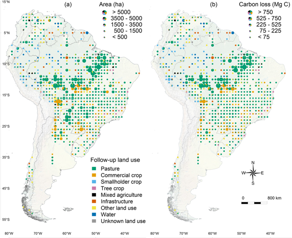
Figure 2. (a) Forest area loss (ha) and (b) related forest carbon losses (Mg C) per follow-up land use from 1990 to 2005, in South America.
Download figure:
Standard image High-resolution imageForest biomass levels in East Brazil, Paraguay and Argentina were much lower than in the Brazilian Amazon (figure 2(b)). This influenced the relative contribution of follow-up land uses for forest carbon losses as compared to deforested area (table 3). For example, commercial crop agriculture proportionally contributed more to deforested area (14.0%) than to forest carbon losses (12.1%) indicating that this follow-up land use, as well as tree crops, occurred more in lower forest biomass eco-zones as compared to pasture, mixed and smallholder crop agriculture, water and infrastructure.
Deforestation drivers at the national level varied in their contribution to deforestation (figure 3, for more detail see table A1 in the appendix). Pasture expansion caused at least 35% or more of forest loss in all countries except in Peru (19.9%) where smallholder cropland (41.9%) was a more dominant driver. In Argentina deforestation caused by commercial cropland (43.4%) was almost as dominant as pasture driven deforestation (44.6%). Commercial crop expansion could also be found in Paraguay (25.5%) and Bolivia (27.2%), while in Colombia smallholder crop and mixed agriculture (23.6% together) was more important for deforestation. In Bolivia one fifth (20.0%) of deforestation was followed up by other land use, mostly wetlands (13.4%) and other wooded land (6.0%). For other land use in Peru (16.2%) most was other wooded land (8.9%) and wetlands (7.3%). In Colombia (12.7%) and Venezuela (13.7%) other land use, mainly other wooded land also played a considerable role in deforestation. In Peru infrastructure was a relatively large driver (5.6%) compared to the other countries, due to mining activities (2.0%) and substantial urban, roads and built-up development (3.7%). Water as a follow-up land use contributed considerably to deforestation in Venezuela (38.2%) due to two large dam projects. In Peru (14.2%) and Bolivia (5.9%) deforestation followed up by water was the result of natural processes such as meandering rivers.
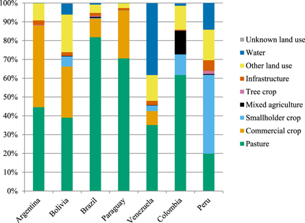
Figure 3. Area proportion of deforestation driver from 1990 to 2005 (%) at the national scale.
Download figure:
Standard image High-resolution imageBrazil emitted the most carbon from 1990 to 2005 (4372 Tg C), followed by Bolivia (488 Tg C), Argentina (297 Tg C) and Colombia (289 Tg C). Paraguay (179 Tg C), Venezuela (174 Tg C) and Peru (170 Tg C) had less forest carbon losses in the same period (table A2 in appendix).
3.2. Trends in annual deforestation and carbon losses per driver from 1990 to 2000 and 2000 to 2005
Annual deforestation increased from 3.62 to 4.46 million ha yr−1 between the periods 1990–2000 and 2000–2005, while the related carbon losses increased from 0.41 to 0.50 Pg C yr−1 (table 4). The increase in carbon losses was partly driven by an increase of forest area loss due to commercial cropland, pasture and other land use. Water, mixed and smallholder crop agriculture, on the other hand, decreased as drivers of deforestation. Not all the increase in carbon losses can be attributed to an increase in forest area loss alone. Pasture (+9.17 Tg C yr−1) and commercial crop expansion (+8.79 Tg C yr−1) caused additional carbon losses by occurring more in higher forest biomass eco-zones in the 2nd period, only minimally countered by other drivers occurring more in lower forest biomass eco-zones (table 4).
Table 4. Estimates of deforested area (103 ha yr−1 (SE)) and related carbon loss (Tg C yr−1 (SE)) per follow-up land use for 1990–2000 and 2000–2005, and the change in carbon loss (Tg C yr−1) in the second period additional to the change in forest area loss.
| 1990–2000 | 2000–2005 | ||||
|---|---|---|---|---|---|
| Follow-up land use | Area | Carbon loss | Area | Carbon loss | Additional change in carbon loss |
| Mixed agriculture | 36 (21) | 5 (3) | 25 (12) | 2 (1) | −0.78 |
| Smallholder crop | 85 (22) | 13 (3) | 58 (13) | 9 (2) | 0.02 |
| Commercial crop | 409 (84) | 37 (7) | 802 (180) | 82 (21) | 8.79 |
| Tree crops | 13 (3) | 1 (0) | 22 (11) | 2 (1) | −0.46 |
| Pasture | 2 642 (224) | 295 (30) | 3 062 (307) | 351 (39) | 9.17 |
| Agriculture total | 3186 (244) | 351 (31) | 3969 (359) | 445 (45) | 16.73 |
| Infrastructure | 64 (25) | 8 (4) | 62 (17) | 7 (2) | −0.31 |
| Other land use | 232 (38) | 27 (5) | 324 (60) | 36 (6) | −2.07 |
| Water | 128 (47) | 18 (7) | 93 (42) | 11 (4) | −2.33 |
| Unknown land use | 9 (7) | 1 (1) | 9 (7) | 1 (1) | −0.04 |
| Other total | 433 (73) | 54 (10) | 489 (77) | 55 (8) | −4.75 |
| Total | 3 619 (261) | 405 (34) | 4 458 (382) | 500 (48) | 11.98 |
Clearly, the spatial distribution of hotspots of deforestation and their change in time has an influence on forest carbon losses. Moving hotspots of the two main deforestation drivers, crop agriculture (commercial and smallholder) (figure 4(a)) and pasture (figure 4(b)), illustrate this effect. Pasture expansion in Brazil occurred more and deeper in the Amazon (especially Rondônia and Pará States) in the 2nd period, and less in lower forest biomass ecoregions of the Cerrado and Mata Atlântica. In Paraguay, pasture expansion into forests moved away from urbanized areas in the first period to mainly the Alto Chaco region in the second period. Hot spots of crop expansion occurred in Mato Grosso State and the lowlands around Santa Cruz in Bolivia mainly in the 2nd period, while in Southern Paraguay crop expansion moved from Alto Paraná Department to central Paraguay. In Peru we see both crop and pasture related deforestation occurring deeper in the Amazon in the second period. In Northern Argentina, pasture and crop expansion occurred mainly near important highways.

Figure 4. Changes in annual rate of deforestation (ha yr−1) followed up by crop agriculture (a) and pasture (b) between the periods 1990–2000 and 2000–2005, in South America.
Download figure:
Standard image High-resolution image
4. Discussion
In this study we quantified proximate drivers of deforestation and related carbon losses in South America between 1990 and 2005. Previous estimates of deforestation ranged from 3.74 to 4.09 million ha yr−1 for the 1990s, and 3.28 to 4.87 million ha yr−1 for (part of) the 2000s (DeFries et al 2002, Hansen et al 2008, 2010, Eva et al 2012, Harris et al 2012, Achard et al 2014, FAO 2015). Previous estimates for carbon losses from deforestation ranged from 306 to 698 Pg C y−1 for the 1990s, and 322 to 845 Pg C yr−1 for (part of) the 2000s (DeFries et al 2002, Baccini et al 2012, Eva et al 2012, Harris et al 2012, Houghton 2012, Achard et al 2014, Tyukavina et al 2015). Our estimates of deforestation and related carbon emissions are of similar magnitude, but comparisons between studies are difficult due to differences in methodology, forest definition, considered time frame and region (Keenan et al 2015). The latter is also the case for previous studies (Hosonuma et al 2012, Houghton 2012) on proximate drivers of deforestation.
Agricultural expansion, in particular pasture, was the most dominant driver of deforestation in South America. Gross carbon losses from forest conversion to pasture were 4 624 Tg C from 1990 to 2005. In the same time frame, carbon losses amounted to 782 Tg C for commercial crop agriculture and 173 Tg C for smallholder crop agriculture. Before the 1990s deforestation was mostly attributed to shifting cultivators and smallholder colonists (Rudel et al 2009). More recent decades saw the rise of large-scale agribusinesses, increasingly producing for international markets, as the main agents of deforestation (Rudel 2007, Rudel et al 2009, Pacheco and Poccard-Chapuis 2012). Our data confirmed this, especially in Brazil, Argentina, Paraguay and Bolivia where large ranches and commercial crop agriculture were the main drivers. In the Andean countries (Peru, Colombia and Venezuela) smallholder and mixed agriculture were still important drivers of deforestation.
Our study shows that the annual rate of deforestation driven by commercial crops doubled in the early 2000s compared to the 1990s. Although much of the increase in deforestation in the early 2000s could be attributed to commercial crop expansion, this driver contributed to only 14% of overall deforestation in South America. Our study identified hotspots of forest conversion for crop agriculture in Mato Grosso State (Brazil), Bolivia, Argentina and Paraguay. Several studies showed that the expansion of commercial crops (e.g. soybean) increased substantially in these regions (Morton et al 2006, Macedo et al 2012, Müller et al 2012, Graesser et al 2015). A large part of this expansion, however, was conversion of pasture and not forests (Graesser et al 2015). Even so, crop expansion still places direct pressure on forests (Morton et al 2006) and can be an indirect driver of land use change by pushing pasture lands forward into the forest frontier (Nepstad et al 2006, Barona et al 2010, Arima et al 2011). These dynamics changed after 2005 when deforestation slowed down in the Amazon, particularly in Mato Grosso State, coinciding with a fall in crop commodity prices and the implementation of policy measures such as improved monitoring and enforcement, and other control actions (Macedo et al 2012, Malingreau et al 2012, Gibbs et al 2015).
Hotspots of pasture- and crop-driven deforestation moved into higher forest biomass eco-zones in the early 2000s which caused additional carbon losses. Efforts to reduce carbon emissions might be in vain when countries only concentrate on reducing the deforested area without taking into account variations in forest biomass. However, beyond carbon emissions, the environmental impact (e.g. biodiversity loss) of high deforestation rates in low-carbon biomes such as the Cerrado in Brazil and the Chaco in Paraguay is considerable. This emphasises the importance of spatial and temporal information, not only on drivers of deforestation but also on biodiversity and other safeguards, in designing effective REDD+ interventions. In this study we used mean forest biomass values per eco-zone to estimate carbon losses as a simple and conservative approach (Langner et al 2014). In reality, however, there are gradations of forest biomass within eco-zones (Saatchi et al 2011, Baccini et al 2012) which might influence the spatial and temporal dynamics of carbon losses from different drivers.
Infrastructure, including urban expansion and roads, contributed little (1.7%) to deforestation as a direct driver. As an indirect driver, however, urbanisation can contribute significantly to deforestation because it changes consumption patterns and increases the demand for agricultural products (DeFries et al 2010). Better road infrastructure in the Amazon opened up the forest frontier and expanded the market for cattle (Rudel 2007). In Peru, infrastructure was a relatively important driver, mostly due to (illegal) mining activities (2.0% of deforestation) which in addition to forest carbon losses also causes other environmental impacts (Swenson et al 2011, Asner et al 2013). The example of Venezuela shows that large infrastructure projects, such as dams, can make a substantial contribution (37.8% of deforestation) to national forest carbon emissions.
Deforestation drivers and their relative importance on the national level emphasise the need to understand drivers to design effective REDD+ policies. Countries have a variety of policy- and incentive-based interventions at their disposal (Angelsen and Brockhaus 2009, Kissinger et al 2012) to affect local to national drivers, which ideally should be adapted to the characteristics of these drivers. For example, countries mostly affected by deforestation due to commercial agriculture might opt for different interventions than countries mostly affected by deforestation due to smallholder agriculture. Most drivers of deforestation originate outside the forest sector which indicates that REDD+ interventions should include non-forest sectors such as the agricultural, urban and mining sectors instead of only focusing on forest interventions such as sustainable forest management. Salvini et al (2014) found that most countries focus more on forest degradation than on deforestation interventions, and that countries with higher quality data on drivers include more non-forest sector interventions (e.g. agricultural intensification) in their REDD+ readiness documents. Clearly, REDD+ countries are struggling with designing effective REDD+ policy interventions partly due to limited understanding of their deforestation drivers.
Unfortunately, our data only covers the timeframe between 1990 and 2005. This limits the applicability for designing up-to-date REDD+ strategies since, as discussed above, the drivers and processes of deforestation in South America have undergone changes after 2005. An important aspect to consider for further research is the influence of the temporal resolution on the follow-up land use. High resolution imagery is usually only available for few points in time within the 1990–2005 timeframe. The immediate follow-up land uses might be missed if a land use transition (e.g. pasture to crop) has occurred between the deforestation event and the closest available high-resolution imagery. In contrast, some land uses only become apparent after some time has passed (e.g. cleared land for urban development). Most REDD+ countries, however, have low capacities for forest monitoring (Romijn et al 2012) and often do not have spatial quantitative data on drivers of deforestation at their disposal (Hosonuma et al 2012). This study provides insight into specific drivers of deforestation that can help REDD+ countries with targeted capacity-building and the stepwise improvement of their national forest monitoring systems to provide more up-to-date and detailed information on drivers of deforestation. In turn this allows for the (re)design of more effective national REDD+ strategies (Salvini et al 2014).
5. Conclusion
In this paper we quantified proximate drivers of deforestation and related carbon losses in South America based on remote sensing time series in a systematic, spatially explicit manner. This contributes to the understanding of drivers of deforestation and related carbon losses at the national and continental level and allows for comparisons across national and regional boundaries. In addition, this spatially explicit quantitative information on deforestation can provide valuable input for statistical analysis and modelling of underlying drivers of deforestation. Our findings can also support the development of national REDD+ interventions and forest monitoring systems.
Our results show the importance of temporal and spatial patterns of deforestation drivers. The future priorities for getting more insight into drivers of deforestation in a REDD+ context lie in expanding the geographical area to all REDD+ focus areas (Central America, Sub-Saharan Africa, South East Asia), in using more recent remote sensing time series, and in using more detailed forest biomass maps to capture spatial forest biomass gradations.
Acknowledgments
The authors gratefully acknowledge the support of NORAD (Grant Agreement #QZA-10/0468) and AusAID (Grant Agreement #46167) for the CIFOR Global Comparative Study on REDD+. The authors would also like to thank German Baldi, Roberto Chavez, and Marcela Velasco-Gomez for lending their regional expertise in reviewing the drivers. In addition, the authors like to acknowledge the input of Sarah Carter, Maria Pereira, Simon Besnard and Arief Wijaya in the development of the methodology.
Appendix A
Table A1. Estimates of deforested area (mean, 103 ha) and standard error (SE, 103 ha) per follow-up land use and country from 1990 to 2005.
| Argentina | Bolivia | Brazil | Colombia | Paraguay | Peru | Venezuela | ||||||||
|---|---|---|---|---|---|---|---|---|---|---|---|---|---|---|
| Follow-up land use | Mean | SE | Mean | SE | Mean | SE | Mean | SE | Mean | SE | Mean | SE | Mean | SE |
| Mixed agriculture | 0 | 0 | 10 | 10 | 229 | 121 | 269 | 263 | 0 | 0 | 4 | 4 | 3 | 3 |
| Smallholder crop agriculture | 0 | 0 | 223 | 136 | 103 | 37 | 233 | 93 | 4 | 4 | 423 | 184 | 50 | 37 |
| Commercial crop agriculture | 1929 | 701 | 1128 | 611 | 3632 | 867 | 0 | 0 | 967 | 522 | 0 | 0 | 125 | 109 |
| Tree crops | 14 | 13 | 1 | 1 | 193 | 68 | 4 | 4 | 0 | 0 | 17 | 15 | 1 | 1 |
| Pasture | 1982 | 523 | 1616 | 472 | 29 949 | 2716 | 1315 | 562 | 2680 | 813 | 201 | 141 | 593 | 215 |
| Infrastructure | 108 | 40 | 81 | 32 | 563 | 320 | 8 | 4 | 45 | 18 | 57 | 28 | 38 | 18 |
| ➢ Urban and Settlements | 3 | 3 | 29 | 25 | 392 | 316 | 1 | 1 | 0 | 0 | 12 | 6 | 25 | 14 |
| ➢ Roads and Built-up | 105 | 40 | 52 | 21 | 95 | 21 | 7 | 4 | 45 | 18 | 25 | 17 | 5 | 3 |
| ➢ Mining | 0 | 0 | 0 | 0 | 76 | 41 | 0 | 0 | 0 | 0 | 20 | 20 | 9 | 9 |
| Other land use | 406 | 214 | 829 | 364 | 1629 | 185 | 270 | 148 | 97 | 30 | 164 | 66 | 231 | 90 |
| ➢ Bare land | 4 | 4 | 6 | 4 | 17 | 15 | 7 | 4 | 0 | 0 | 0 | 0 | 28 | 28 |
| ➢ Other wooded land | 163 | 57 | 247 | 68 | 1495 | 180 | 232 | 135 | 92 | 29 | 90 | 58 | 161 | 62 |
| ➢ Grass & herbaceous | 235 | 197 | 19 | 13 | 34 | 19 | 14 | 12 | 2 | 2 | 0 | 0 | 41 | 34 |
| ➢ Wetlands | 4 | 3 | 557 | 346 | 83 | 31 | 17 | 11 | 3 | 3 | 74 | 30 | 1 | 1 |
| Water bodies | 4 | 3 | 243 | 102 | 300 | 89 | 26 | 14 | 4 | 3 | 143 | 50 | 646 | 402 |
| ➢ Natural | 4 | 3 | 243 | 102 | 253 | 88 | 26 | 14 | 4 | 3 | 143 | 50 | 8 | 5 |
| ➢ Man-made | 0 | 0 | 0 | 0 | 47 | 12 | 0 | 0 | 0 | 0 | 0 | 0 | 638 | 402 |
| Unknown land use | 0 | 0 | 12 | 10 | 2 | 2 | 5 | 3 | 0 | 0 | 0 | 0 | 1 | 1 |
| Total | 4441 | 989 | 4142 | 943 | 36 599 | 3008 | 2129 | 650 | 3798 | 921 | 1010 | 264 | 1689 | 586 |
Table A2. Estimates of forest carbon losses (mean, Mg C) and standard error (SE, Mg C) per follow-up land use and country from 1990 to 2005.
| Argentina | Bolivia | Brazil | Colombia | Paraguay | Peru | Venezuela | ||||||||
|---|---|---|---|---|---|---|---|---|---|---|---|---|---|---|
| Follow-up land use | Mean | SE | Mean | SE | Mean | SE | Mean | SE | Mean | SE | Mean | SE | Mean | SE |
| Mixed agriculture | 0 | 0 | 1235 | 1232 | 22 521 | 12 357 | 40 119 | 39 454 | 0 | 0 | 738 | 737 | 325 | 324 |
| Smallholder crop agriculture | 0 | 0 | 27 155 | 16 068 | 13 557 | 4823 | 34 802 | 13 926 | 225 | 223 | 70 760 | 31 848 | 7714 | 5867 |
| Commercial crop agriculture | 127 523 | 47 503 | 135 073 | 79 944 | 416 421 | 117 043 | 0 | 0 | 50 349 | 27 204 | 0 | 0 | 11 949 | 10 768 |
| Tree crops | 962 | 930 | 78 | 77 | 15 531 | 4813 | 234 | 234 | 0 | 0 | 2195 | 2025 | 139 | 138 |
| Pasture | 129 699 | 37 173 | 174 770 | 51 130 | 3605 826 | 384 314 | 180 656 | 84 179 | 121 185 | 36 091 | 33 394 | 24 346 | 59 368 | 21 417 |
| Infrastructure | 7121 | 2983 | 7847 | 3599 | 79 345 | 48 346 | 1019 | 513 | 2108 | 820 | 9876 | 4830 | 4063 | 1754 |
| ➢ Urban and Settlements | 230 | 218 | 3864 | 3354 | 56 699 | 47 904 | 116 | 114 | 0 | 0 | 2102 | 954 | 2691 | 1421 |
| ➢ Roads and Built-up | 6890 | 2956 | 3983 | 1426 | 11 315 | 2764 | 903 | 503 | 2108 | 820 | 4324 | 2903 | 451 | 287 |
| ➢ Mining | 0 | 0 | 0 | 0 | 11 332 | 6197 | 0 | 0 | 0 | 0 | 3450 | 3449 | 921 | 913 |
| Other land use | 31 893 | 16 896 | 108 734 | 48 763 | 184 727 | 23 604 | 29 922 | 15 634 | 4666 | 1400 | 28 139 | 11 462 | 26 242 | 9973 |
| ➢ Bare land | 325 | 340 | 634 | 477 | 2481 | 2272 | 834 | 580 | 0 | 0 | 0 | 0 | 2746 | 2729 |
| ➢ Other wooded land | 12 649 | 4379 | 31 603 | 9138 | 173 326 | 23 307 | 26 730 | 14 292 | 4407 | 1364 | 15 446 | 10 058 | 17 192 | 6609 |
| ➢ Grass and herbaceous | 18 587 | 15 634 | 2025 | 1481 | 2032 | 986 | 1336 | 1239 | 98 | 82 | 0 | 0 | 6160 | 5098 |
| ➢ Wetlands | 331 | 235 | 74 472 | 46 463 | 6889 | 2352 | 1022 | 627 | 161 | 132 | 12 693 | 5290 | 143 | 143 |
| Water bodies | 289 | 201 | 31 967 | 13 641 | 34 173 | 10 731 | 2292 | 1130 | 162 | 131 | 24 666 | 8647 | 63 690 | 39 629 |
| ➢ Natural | 289 | 201 | 31967 | 13 641 | 28 914 | 10 656 | 2292 | 1130 | 162 | 131 | 24 666 | 8647 | 769 | 496 |
| ➢ Man-made | 0 | 0 | 0 | 0 | 5259 | 1434 | 0 | 0 | 0 | 0 | 0 | 0 | 62 922 | 39 647 |
| Unknown land use | 0 | 0 | 1536 | 1218 | 298 | 263 | 448 | 280 | 0 | 0 | 0 | 0 | 156 | 154 |
| Total | 297 486 | 68 154 | 488 395 | 117 738 | 4372 400 | 426 070 | 289 492 | 96 679 | 178 695 | 42 935 | 169 769 | 45 669 | 173 647 | 58 141 |