
Abstract
Analysis of single forcing runs from CMIP5 (the fifth Coupled Model Intercomparison Project) simulations shows that the mid-twentieth century temperature hiatus, and the coincident decrease in precipitation, is likely to have been influenced strongly by anthropogenic aerosol forcing. Models that include a representation of the indirect effect of aerosol better reproduce inter-decadal variability in historical global-mean near-surface temperatures, particularly the cooling in the 1950s and 1960s, compared to models with representation of the aerosol direct effect only. Models with the indirect effect also show a more pronounced decrease in precipitation during this period, which is in better agreement with observations, and greater inter-decadal variability in the inter-hemispheric temperature difference. This study demonstrates the importance of representing aerosols, and their indirect effects, in general circulation models, and suggests that inter-model diversity in aerosol burden and representation of aerosol–cloud interaction can produce substantial variation in simulations of climate variability on multi-decadal timescales.
Export citation and abstract BibTeX RIS

Content from this work may be used under the terms of the Creative Commons Attribution 3.0 licence. Any further distribution of this work must maintain attribution to the author(s) and the title of the work, journal citation and DOI.
1. Introduction
Atmospheric aerosols exert both a direct (through modification of radiative transfer) and indirect (through aerosol–cloud interactions) effect on climate. Present day global aerosol emissions are substantially greater than in 1850, but the historical changes in emissions have neither been linear, nor uniform across the globe. Of particular interest has been the potential role of anthropogenic aerosol in producing 'hiatuses' in the global temperature record, for example the cooling in global-mean, near-surface temperature during the 1950s and 1960s (e.g. Tett et al 2002, Stott et al 2006). Additionally, the driver of the current temperature hiatus since 2000 is still a topic of debate, and it is possible that aerosol is important here too (e.g. Meehl et al 2011, Hunt 2011, Kaufmann et al 2011). Overall, aerosol produces a negative radiative forcing of climate, leading to a cooler surface and a consistent decrease in global-mean precipitation. The indirect effect may account for almost all aerosol cooling in models (Levy et al 2013), and for 2/3 of the aerosol driven decrease in precipitation in GFDL-CM3 (Levy et al 2013). However, this is model dependent. For example, Shindell et al (2012) found that including the indirect effect in the CMIP3 version of GISS-ER made little difference. The importance of the aerosol indirect effect in regional climate change is also a topic of debate (e.g. Booth et al 2012, Zhang et al 2013).
In comparison to the climate models used in the third Coupled Model Intercomparison Project (CMIP3), those from the most recent intercomparison, CMIP5, generally have improved representation of aerosol–cloud interactions. Specifically, many models now include at least the first indirect effect of sulfate aerosol (table 1). Many CMIP5 models also have interactive schemes for aerosol species; models may use the same emission inputs for aerosols and aerosol pre-cursors, but simulate diverse aerosol loadings in the atmosphere. Thus it is important to understand the role of aerosol and aerosol–cloud influences on climate and climate simulations at a variety of temporal and spatial scales. The CMIP5 model simulations, with their variation in aerosol representations, offer a unique opportunity to examine these issues. In this study we consider the response to historical aerosol forcing of global-mean near-surface temperature, the inter-hemispheric temperature difference, and land-mean precipitation. We use ensembles of CMIP5 models with and without representations of the indirect effect of sulfate aerosol, single forcing experiments, and employ the technique of Ensemble Empirical Mode Decomposition (EEMD), to consider multi-decadal scale non-linear trends.
Table 1. CMIP5 models used in this study. Models without a representation of the indirect effect of sulfate aerosol are shown in italics. Models in boldface are used in the ensemble of single forcing runs. Numbers shown in parentheses give the number of ensemble members used in single forcing calculations: (GHG only, natural only, anthropogenic aerosol only). E1 anthropogenic emissions are taken from the Lamarque et al (2010) emissions inventory. E1a is the same, but with black carbon increased uniformly by 25% and organic aerosol increased by 50% (Rotstayn et al 2012). C1 anthropogenic concentrations are the (Meehl et al 2006) inventory; C2 are the Collins et al (2006) climatology; C3 is from AEROCOM (Penner et al 2006); C4 are concentrations from HAC-v1 (Kinne et al 2013); C5 is decadal-average monthly aerosol concentration derived using the CAM-Chem model, driven by the Lamarque et al (2010) emissions.
| Institute | Model | Ensemble | First indirect | Second indirect | Ant | Reference |
|---|---|---|---|---|---|---|
| CCCma | CanESM2 | 5(5, 5, 5) | Y | N | E1 | von Salzen et al (2013) |
| CNRM-CERFACS | CNRM-CM5 | 1 | Y | N | E1 | Szopa et al (2013) |
| Voldoire et al (2012) | ||||||
| CSIRO-QCCCE | CSIRO-Mk3.6.0 | 5(5, 5, 5) | Y | N | E1a | Rotstayn et al (2012) |
| NOAA GFDL | GFDL-CM3 | 1 | Y | N | E1 | Donner et al (2011) |
| MOHC | HadGEM2-CC | 1 | Y | Y | E1 | Bellouin et al (2007) |
| Collins et al (2011) | ||||||
| MOHC | HadGEM2-ES | 4(4, 4, 4a) | Y | Y | E1 | Bellouin et al (2007) |
| Collins et al (2011) | ||||||
| INM | INMCM4 | 1 | Y | N | C1 | Volodin (2013) |
| IPSL | IPSL-CM5A-LR | 3(3, 3, 1) | Y | N | E1 | Dufresne et al (2013) |
| IPSL | IPSL-CM5A-MR | 1 | Y | N | E1 | Dufresne et al (2013) |
| NCC | NorESM1-M | 1(1, 1, 1) | Y | Y | E1 | Iversen et al (2012) |
| MIROC | MIROC5 | 1 | Y | Y | E1 | Watanabe et al (2010) |
| MIROC | MIROC-ESM | 1 | Y | Y | E1 | Watanabe et al (2011) |
| MIROC | MIROC-ESM-CHEM | 1 | Y | Y | E1 | Watanabe et al (2011) |
| MRI | MRI-CGCM3 | 1 | Y | N | E1 | Yukimoto et al (2012) |
| Yukimoto (2013) | ||||||
| BCC | BCC-CSM1.1 | 1 | N | N | C2 | Wu et al (2010) |
| BNU | BNU-ESM | 1 | N | N | E1 | Ji (2013) |
| NSF-DOE-NCAR | CESM1-BGC | 1 | N | N | E1 | Strand (2013) |
| NSF-DOE-NCAR | CESM1-CAM5 | 1 | N | N | E1 | Strand (2013) |
| NSF-DOE-NCAR | CESM1-FASTCHEM | 1 | N | N | E1 | Strand (2013) |
| NSF-DOE-NCAR | CESM1-WACCM | 1 | N | N | E1 | Strand (2013) |
| ICHEC | EC-Earth | 1 | N | N | C3 | Hazeleger et al (2012) |
| FIO | FIO-ESM | 1 | N | N | E1 | Song (2013) |
| NOAA GFDL | GFDL-ESM2G | 1 | N | N | E1 | Dunne et al (2012) |
| NOAA GFDL | GFDL-ESM2M | 1 | N | N | E1 | Dunne et al (2012) |
| MPI-M | MPI-ESM-LR | 1 | N | N | C4 | Stevens et al (2013) Kinne et al (2013) |
| NCAR | NCAR-CCSM4 | 1 | N | N | C5 | Meehl et al (2012) |
aThe difference between the historical simulation and a historical simulation with anthropogenic aerosol fixed at 1860 levels.
2. Data and methods
The CMIP5 models used in this study, their representation of aerosol effects, and their aerosol inventories, are shown in table 1. 'All forcing' model simulations include a representation of the major known climate forcings, including greenhouse gases, ozone, tropospheric aerosol, volcanic aerosol, and solar variations. Observed forcing is used in the historical period (1850–2005), and the majority of models considered here draw aerosol emissions from the same inventory (table 1). A subset of models, highlighted in boldface in table 1, also provide single forcing runs for the historical period: greenhouse gas only, natural (volcanic and solar) only, anthropogenic aerosols (sulfate, black carbon, and organic carbon) only. These models will be used to identify the primary drivers of historical trends (section 3).
In order to investigate the role of the indirect effect in historical trends and variability (section 4), models have been divided into two ensembles: those with and without a representation of the indirect effect of sulfate aerosol (named SA and SD respectively, following CMIP5 metadata convention). The aerosol indirect effect is comprised of a first and second effect. The first indirect effect is the response of cloud droplet radius and cloud droplet number concentration to aerosol concentration, while the second indirect effect is a resultant impact on cloud lifetime, depth, and liquid water content. Models included in the indirect ensemble, SA, have at least a representation of the first indirect effect. Many also include the second indirect effect. The remaining models, SD, only represent the direct effect of sulfate aerosol (table 1). The all forcing historical simulations are used for this analysis as there are insufficient single forcing runs currently available within the CMIP5 database.
Observational data sets are required to evaluate the performance of models. In this study CRUTS3.1.1 (Harris et al 2013) and HadCRUT4 (Morice et al 2012) have been used. CRUTS3.1.1 compiles land-based observations of near-surface temperature and gauge-based observations of precipitation from up to 4000 stations onto a 0.5° × 0.5° grid. Data are available from 1901 to 2009. HadCRUT4 is a global data set of near-surface temperature derived from the combination of CRUTEM4 and HadSST3 data. Data are presented as an anomaly relative to 1961–90, on a 5° × 5° grid from 1850 to the present. Data for 100 ensemble members are available, which sample the uncertainty arising from non-climatic factors such as changes in measurement practices. The median of these has been used here.
Although there are observations of aerosol optical depth spanning the twentieth century, they are typically comprised of local, short-term records, that cannot be used for long-term global analysis (Holben et al 2001). In recent decades, remote sensing data sets have improved the spatial coverage of observations. However, remote sensing of aerosol optical depth is complex, and assumptions about aerosol properties may lead to spurious trends (Mishchenko et al 2012). New measurements from SeaWiFS provide global coverage, and minimize the uncertainties associated with calibration (Hsu et al 2012). The annual-mean global-mean aerosol optical depth at 550 nm from a subset of CMIP5 models is shown in figure 1, alongside the SeaWiFS observed optical depth. Although the CMIP5 mean is in good agreement with the observed values, there is considerable inter-model spread, despite the majority of models having used the (Lamarque et al 2010) emissions inventory.

Figure 1. Annual-mean global-mean aerosol optical depth at 550 nm from CMIP5 models (blue) for 1870–2004. The CMIP5 multi-model mean is shown in black. SeaWiFS (green) values are shown for 1998–2007. Note that some CMIP5 models do not represent stratospheric volcanic eruptions as a change in aerosol optical depth.
Download figure:
Standard image High-resolution image2.1. Empirical mode decomposition
Historical time series of temperature and precipitation are non-linear. Empirical mode decomposition (EMD) is an algorithm used to decompose a time series into a set of intrinsic mode functions (IMFs), which each describe a given oscillatory mode of the data. IMFs must have a single zero crossing between two extrema, and a local mean of zero (Huang et al 1998). IMFs are sequentially extracted from the time series, from the highest frequency to the lowest, until only a residual remains. The number of IMFs identified is typically lnN, where N is the number of data points (Wu et al 2007). High-order IMFs of global-mean annual-mean near-surface temperature are shown in figure 2(a). Ensemble empirical mode decomposition (EEMD) uses the ensemble mean of the IMFs from the product of the time series of interest and a white noise series of the same length. The use of noise in this manner assists in the separation of different timescales in noisy data, but does not contribute to the final IMFs (Wu and Norden 2009). The residual from the decomposition process describes the long-term trend in the data, where the trend is defined as the instantaneous mean of the time series. Non-linear trends have been defined here as the sum of the residual and the last IMF in order to filter out high frequency oscillatory modes whilst retaining inter-decadal variability. Figure 2(b) shows an example of the non-linear trend in global-mean annual-mean near-surface temperature. EEMD has successfully been applied to climate data in several previous studies (e.g. Chang et al 2011, Lee and Ouarda 2011, Franzke 2009, Huang et al 2008, Wu et al 2007, McDonald et al 2007, and Duffy 2004).
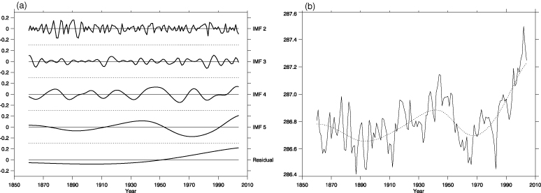
Figure 2. (a) High-order IMFs and the residual of global-mean annual-mean near-surface temperature from HadGEM2-ES. (b) The sum of the last IMF, the residual, and the mean (dashed), superimposed on the original time series (solid).
Download figure:
Standard image High-resolution image3. Drivers of trends
Single forcing runs are available for only a subset of CMIP5 models (shown in bold in table 1). These are used to understand the forcing mechanisms driving the observed trends in temperature and precipitation. Non-linear trends in the single forcing runs are shown in figure 3 for global-mean annual-mean near-surface temperature and the inter-hemispheric temperature difference. Land-mean annual-mean precipitation (to allow comparison with observational data sets) is shown in figure 4. Ensemble means for each run are shown alongside the all forcing run, adjusted to 1900 values, with shading to indicate the absolute range of solutions from the component simulations at key points in the time series. The number of ensemble members from each model for each simulation is shown in table 1.
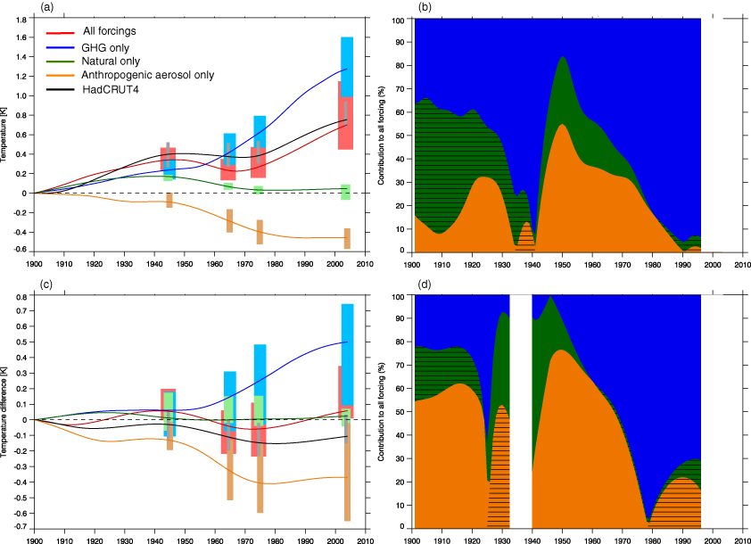
Figure 3. Non-linear trends (where the trend is the sum of the last IMF and the residual) from single forcing runs and observations for (a) global-mean annual-mean near-surface temperature; (c) annual-mean inter-hemispheric temperature difference. For model data, solid lines show the ensemble mean for each run, shading shows the absolute range of the instantaneous values from individual ensemble members (shown in bold in table 1) at the designated time. For HadCRUT4, the solid line shows the median of 100 ensemble members, and shading shows uncertainty resulting from measurement and sampling error, and coverage uncertainty (see Morice et al (2012) for further details of the uncertainty). Contributions from anthropogenic aerosol (sulfate, black carbon, and organic carbon), natural (solar and volcanic), and greenhouse gas forcing to the rate of change in (b) global-mean annual-mean near-surface temperature; (d) annual-mean inter-hemispheric temperature difference. No data is shown when the linear sum of the single forcing response is a poor approximation of the all forcing experiment.
Download figure:
Standard image High-resolution image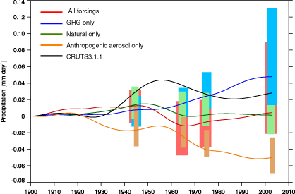
Figure 4. Non-linear trends from single forcing runs and observations for land-mean annual-mean precipitation.
Download figure:
Standard image High-resolution image3.1. Temperature
Observations of global-mean annual-mean near-surface temperature from HadCRUT4 analysed using the EEMD technique (figure 3(a)) show a warming until 1945, a cooling until 1975, and finally a warming until 2000. The turning points in this time series are well matched by the ensemble mean all forcing experiment, although the change in trend during the 1945–1975 period has a slightly larger amplitude in the modelled time series. Temperature increases throughout the greenhouse gas (GHG) only run (figure 3(a)), with the rate of change increasing from 1955. An increase in temperature is also seen in the natural forcing run before 1940, which is followed by a decrease to 1970, before the temperature stabilizes. Temperature predominantly decreases throughout the anthropogenic aerosol only run: after a small increase in the 1930s the trend is negative, with the rate of decrease steadily increasing from 1945, before levelling off in the 1980s. The decrease in temperature in the all forcings run between 1950 and 1970 therefore occurs despite an accelerating increase due to GHG changes. Hence, it follows that the cooling seen in both the natural forcings and anthropogenic aerosol forcing runs combine to drive an overall decrease in temperature in this period.
For global-mean near-surface temperature, the sum of the anomalies due to GHG, natural, and anthropogenic aerosol only forcing gives a good reproduction of the anomaly from the all forcing run. The sum of the instantaneous gradients from the single forcing simulations are also a good approximation for the gradient of the all forcings simulation. Although multiple-linear regression cannot be used to identify drivers in this case because the GHG and aerosol forcing are co-varying, these linear relationships allow the contribution of each of GHG, natural, and anthropogenic aerosol forcing to the temperature tendency to be quantified. The percentage contribution from each forcing component to the all forcings gradient with time is shown in figure 3(b) for annual-mean global-mean near-surface temperature. A positive and negative trend are considered to have equally weighted contributions, so the sum of contributions to the all forcing tendency is always 100%. Using this method, anthropogenic aerosol forcing alone accounts for >50% of the variation in temperature in the decade centred on 1950. In excess of 50% of the variation is explained by the combination of natural and anthropogenic aerosol forcing from 1945 to 1965, with at least 35% from anthropogenic aerosol forcing throughout that whole period. The anthropogenic aerosol forcing contribution to temperature trends decreases rapidly during the 1970s as anthropogenic aerosol concentrations plateau (figure 1).
3.2. Inter-hemispheric temperature difference
Previous studies have identified sulfate aerosol as a driver of the observed trend in the inter-hemispheric temperature difference (Tett et al 2002, Stott et al 2006, Chang et al 2011). However, Thompson et al (2010) have recently suggested that the trend may in fact be due to abrupt changes in sea surface temperature.
The non-linear trend in the annual-mean inter-hemispheric temperature difference is shown in figure 3(c). As the response to natural forcing tends to be quite hemispherically symmetric, there is only a small signal in the natural forcing experiment. Land–ocean warming contrasts cause the Northern Hemisphere to warm faster than the Southern Hemisphere in response to increased GHG concentrations, and this contrast is reflected strongly in the GHG only experiment. Emissions of anthropogenic aerosols are greater in the Northern Hemisphere, and, because of their short atmospheric residence time, this asymmetry is reflected in the associated temperature changes. The Northern Hemisphere cools more than the Southern Hemisphere in response to increased anthropogenic aerosol, resulting in a negative temperature difference, with a maximum magnitude in the early 1970s. The temperature difference in the all forcings run shows a near cancellation between the anthropogenic aerosol and GHG influences. However, the inter-decadal variability seen in the anthropogenic aerosol run is clearly reflected in the all forcings case.
The temperature difference decreases between 1945 and 1970 in the all forcings run and HadCRUT4, by comparable amounts. However, the modelled rate of decrease is greater. The models also slightly overestimate the rate of increase in the temperature difference in recent decades. There are many possible explanations for this difference, including an overestimate of the magnitude of the aerosol indirect effect, and different representations of land use change.
Figure 3(d) shows that the change in inter-hemispheric temperature difference is primarily driven by anthropogenic aerosol forcing prior to 1970. In recent decades, anthropogenic aerosol accounts for over 20% of the rate of change in the inter-hemispheric temperature difference. Recent Northern Hemisphere decreases in sulfate concentrations mean that aerosol now acts to decrease the difference. Both the positive and negative trends simulated by the models since the mid-twentieth century have a larger magnitude than the trends seen in the observations. It is possible that this divergence is caused, in part, by an overestimate of the aerosol effects in the models used in our single forcing subset.
3.3. Precipitation
Considering land-only grid points facilitates comparison between observed (CRUTS3.1.1) and modelled precipitation. Land-mean annual-mean precipitation is shown in figure 4. A pattern similar to the non-linear trends in global-mean temperature (figure 3) can be seen, with a dip in the all forcings run coincident with a pronounced decrease in precipitation in the anthropogenic aerosol and natural forcing only simulations. Unlike global-mean near-surface temperature, linear additivity of the single forcing runs does not hold for precipitation, so it is difficult to quantify the effect of a single forcing agent on the overall trend. However, the coincident negative trends in the natural and anthropogenic aerosol only, and all forcing runs in the mid-twentieth century still imply an important role from non-GHG forcing in this period.
While the models show the correct tendency, the decrease in precipitation in the mid-twentieth century occurs too quickly compared the observations. The observations also show a large increase in precipitation in the first half of the twentieth century that is not captured by the models.
Masking modelled and observed precipitation with a grid based on the location of temporally consistent observations has been shown to improve the agreement between models and observations (Balan Sarojini et al 2012). This is the case for raw data. However, masking considerably increases the noise in the time series. Filtering methods for identifying inter-decadal variability can be very sensitive to the differences in noisy data, and the resultant trends do not always produce an intuitive representation of the data. As we aim to use model data to identify drivers of the historical trend, rather than to produce a rigorous comparison of observed and modelled time series, masking has not been used here.
4. The importance of the representation of the aerosol indirect effect
The constituent models of the single forcing ensembles used here all represent the indirect effect of sulfate aerosol to some degree. However, many models in CMIP3, and some in CMIP5, include only the direct effect. If the indirect effect is indeed responsible for a large part of the total aerosol forcing, we might expect models including the indirect effect to compare more favourably with multi-decadal scale variations in observations.
Figure 5(a) shows a clear long-term positive trend in surface air temperature, superimposed with some decadal variability. The ensemble mean of models with a representation of the indirect effect, SA, (heavy blue line) shows temperature increasing from c1890 to c1950, followed by a decrease until c1970 when the positive trend returns. This matches the temporal pattern seen in HadCRUT4, and the all forcing run from the single forcing ensemble, suggesting that this temporal pattern is insensitive to model selection. While the SA ensemble has a local maximum at 1950, the SD ensemble (those models with a representation of the direct effect only) has a point of inflection here. The smaller positive trends, and larger negative trends, in temperature in the SA ensemble are likely to be reflections of the inclusion of the indirect effect, which results in a net cooling and offsets some of the greenhouse gas induced warming since 1965. The negative trends seen in 1950–1970 are temporally coincident with large positive trends in aerosol optical depth (figure 1). If indirect aerosol effects are key to reproducing the negative trends, then it follows that larger magnitude negative trends in the SA ensemble, and larger magnitude positive trends in the SD ensemble, would be expected, as is seen in figure 5.

Figure 5. Non-linear trends in (a) global-mean annual-mean near-surface temperature; (b) global-mean annual-mean precipitation; (c) annual-mean inter-hemispheric temperature difference; (d) land-mean annual-mean precipitation. Heavy lines show the ensemble mean, thin lines show one ensemble member from the individual models.
Download figure:
Standard image High-resolution image
It can be seen in figure 5(b) that, compared to near-surface temperature, there is greater uncertainty about the sign of the long-term trend in global-mean precipitation. However, both ensemble means show a local maximum in the mid 20th century and positive trends since c1970, although there is far less confidence in this trend than the temperature trend in figure 5(a).
Land-mean annual-mean precipitation since 1900 is shown in figure 5(d) for the SA and SD ensembles, alongside observations from CRUTS3.1.1. Variability in individual models is greater in the land-only case than in the global-mean, but the ensemble means show a similar temporal pattern. The decease in precipitation between 1940 and 1970 is larger in the SA ensemble, and the increase since 1960 is larger in the SD case, consistent with the temperature trends in figure 5(a). As was shown in figure 4, there is some disagreement between the modelled and observed turning points.
Figure 5(c) shows the inter-hemispheric temperature difference. The SA ensemble mean is again comparable to the single forcing ensemble. The SA models overestimate the trend in recent decades compared to observations. The SD ensemble mean has a reduced amplitude compared to SA, and a poor representation of the temporal structure, especially prior to 1920. Chang et al (2011) showed that, for CMIP3 models, a representation of the indirect effect resulted in larger trends that were in better agreement with observations. This appears also to be the case for the CMIP5 ensemble means. The smaller amplitude of variability in the SD mean in this case may be due, at least in part, to the poor consistency across models compared to the SA ensemble.
5. Conclusions
The EEMD technique used here demonstrates, at high temporal resolution, that the modelled decrease in global-mean annual-mean temperature between 1950 and 1970 was due to a combination of natural and anthropogenic aerosol forcing, as has been previously suggested (e.g. Tett et al 2002, Stott et al 2006). We also show that CMIP5 models with a representation of the aerosol indirect effect better reproduce observations in this period. This suggests that the observed temperature trend between 1950 and 1970 is likely to be due primarily to a combination of anthropogenic aerosol and natural forcing. Although the trends, and the signal to noise ratio, are smaller for land-precipitation, this also appears to be the case for the concurrent decrease in precipitation.
Anthropogenic aerosol forcing accounts for over a third of the modelled multi-decadal variations in global-mean annual-mean near-surface temperature in the mid-twentieth century. The inter-hemispheric temperature difference is more closely related to anthropogenic aerosol, as we would expect, with aerosol forcing accounting for over 50% of the variability before 1970, and in excess of 70% in the decade either side of 1950. An absence of linear additivity in the case of precipitation means that the contribution to the overall trend from individual forcings cannot be quantified in this manner. However, it is evident that the combination of natural and anthropogenic aerosol forcing determines the sign of the trend in land-precipitation in the mid-twentieth century.
CMIP5 models that include a representation of the indirect effects of sulfate aerosol are able to better reproduce inter-decadal variability in historical near-surface temperature. Models with a representation of only the direct effect of aerosol underestimate the variability in the mid-twentieth century in particular. Models including a representation of the aerosol indirect effect are also able to represent more of the inter-decadal variability in land-only precipitation compared to those without. However, they underestimate the amplitude, and show disagreement in the timing of turning points in the precipitation timeseries compared to CRUTS3.1.1.
It is suggested that in the future there will be strong reductions in aerosol cooling, and that these may be substantial for aggressive mitigation cases (Kloster et al 2010, Johns et al 2011, Chalmers et al 2012). This would lead to an additional warming influence. The results shown here suggest that changes in aerosols can strongly influence the decadal timescale variations in global-mean climate, and especially inter-hemispheric temperature difference, and that models with an indirect effect of sulfate aerosol will likely produce more reliable predictions of near-future climate change. However, the CMIP5 models demonstrate considerable diversity in aerosol burden and sensitivity of clouds to aerosols, and until this diversity is understood, a large uncertainty will be inherent in predictions of near-future climate change, even outside of the considerable uncertainty in likely changes in aerosol emissions.
Acknowledgments
This work is supported by the PAGODA project of the Changing Water Cycle programme of the UK Natural Environment Research Council (NERC) under grant NE/I006672/1. NJD was supported by the joint DECC/DEFRA Met Office Hadley Centre Climate Programme (GA0110).
We acknowledge the World Climate Research Programme's Working Group on Coupled Modelling, which is responsible for CMIP, and we thank the climate modelling groups for producing and making available the model output listed in table 1. For CMIP the US Department of Energy's Program for Climate Model Diagnosis and Intercomparison provides coordinating support and led development of software infrastructure in partnership with the Global Organization for Earth System Science Portals.
We also thank the British Atmospheric Data Centre (BADC) for providing access to their CMIP5 data archive, and two anonymous reviewers for their helpful feedback.