
Abstract
In this letter, we investigate the effects of crop yield and livestock feed efficiency scenarios on greenhouse gas (GHG) emissions from agriculture and land use change in developing countries. We analyze mitigation associated with different productivity pathways using the global partial equilibrium model GLOBIOM. Our results confirm that yield increase could mitigate some agriculture-related emissions growth over the next decades. Closing yield gaps by 50% for crops and 25% for livestock by 2050 would decrease agriculture and land use change emissions by 8% overall, and by 12% per calorie produced. However, the outcome is sensitive to the technological path and which factor benefits from productivity gains: sustainable land intensification would increase GHG savings by one-third when compared with a fertilizer intensive pathway. Reaching higher yield through total factor productivity gains would be more efficient on the food supply side but halve emissions savings due to a strong rebound effect on the demand side. Improvement in the crop or livestock sector would have different implications: crop yield increase would bring the largest food provision benefits, whereas livestock productivity gains would allow the greatest reductions in GHG emission. Combining productivity increases in the two sectors appears to be the most efficient way to exploit mitigation and food security co-benefits.
Export citation and abstract BibTeX RIS

Content from this work may be used under the terms of the Creative Commons Attribution-NonCommercial-ShareAlike 3.0 licence. Any further distribution of this work must maintain attribution to the author(s) and the title of the work, journal citation and DOI.
1. Introduction
Agriculture is a major contributor to greenhouse gas (GHG) emissions through crop cultivation, livestock, and land use change. These sources altogether account for about one-third of total anthropogenic GHG emissions, and four-fifths of them are located in developing countries [1, 2]. Various mitigation strategies exist at different costs [3], but would require either change in consumption patterns or some constraints on agricultural activities, with some implications for food supply [4]. Investing in productivity improvement is usually presented as an efficient way to simultaneously achieve GHG emission reduction and ensure food availability, one of the key pillars of food security [5–7].
Major productivity gaps remain that could be exploited to supply more food on existing agricultural land and at lower costs [8]. Increasing land productivity would, in particular, relax the pressure from land conversion on current deforestation frontiers and help avoid large emissions and biodiversity losses [9]. Indeed, past crop yield increases are estimated to have spared 85% of cropland over 50 years and avoided some 590 GtCO2 of land-use-related GHG emissions [10]. On the livestock side, feed productivity increase is generally perceived as the most effective mitigation option [11], as add-on technologies (anti-methanogens, digesters) can only achieve limited levels of abatement [12].
However, the effect of agricultural productivity increase on climate change mitigation can be ambiguous. First, investments focusing on input intensification only increase productivity of some factors, and can worsen pressure on the environment. Fertilizer application, for instance, can lead to additional nitrous oxide emissions with a high radiative forcing power [13], and machinery used for tillage, harvest, or irrigation burns extra fuel [14]. In addition, even when production increase is reached through resource-saving total factor productivity (TFP) gains, decrease in prices stimulates further demand and consequently production and input use, a phenomenon commonly referred to as the rebound effect [15, 16]. Indeed, empirical studies find mixed results when looking at local land sparing effects in regions where yields were substantially increased [17]. Overall, the level of environmental and food supply benefits that can arise from land productivity increases is revealed to be highly dependent on which technology and which investment scheme are chosen from among the large array possible [18].
In this letter, we present an overview of the implications from different productivity developments in agriculture with respect to climate change mitigation and food supply in developing countries. Our analysis relies on a comprehensive agriculture and land use partial equilibrium model covering the major GHG emission sources and agricultural product markets. We study contrasting scenarios of crop yield and livestock feed conversion efficiency development with stagnation or catching up at levels of more advanced countries. Three different productivity pathways are looked at to achieve these yield levels; two rely mainly on partial productivity gains with input intensification with or without fertilizer increase, and one on total factor productivity gains, with a higher effect on production prices. Our scenarios are presented in detail in section 2, followed by a presentation of the model and GHG accounting methods. Results of the scenarios for future food availability and GHG emissions, and the various trade-offs and synergies are analyzed in section 4; the implications are discussed in the last part of the letter.
2. Exploring different productivity futures
2.1. Baseline assumptions
We draw our analysis from a reference situation describing a plausible future up to 2050 for different regions of the world. Population and GDP changes follow the assumptions from scenario SSP2 ('Middle of the Road') of the Shared Socioeconomic Pathways developed by the climate change community [19]. Patterns of future food demand are calibrated on FAO projections [20]. Yield growth for crops and livestock are assumed to follow recent historical trends, which are extended linearly to 2050. In the case of crops, such trends are derived from analysis of past FAOSTAT yields between 1980 and 2010. Fertilizer use is assumed to increase with crop yield with an elasticity of 0.75, following the world average trend observed over the last 30 years. For livestock, we rely on the feed conversion efficiency information from Bouwman et al [21] and apply it to the different grass-based and mixed systems in the model. For both crops and livestock, we consider in the baseline that input and factors other than land and feed are increased and production costs per unit of output are only marginally affected. More details on the baseline are available in the supplementary information (SI, available at stacks.iop.org/ERL/8/035019/mmedia).
2.2. Yield scenarios and productivity pathways
Four different yield scenarios and three productivity pathways are considered around the baseline (scenario 'TREND' with pathway 'High-Input'). Yield scenarios only modify crop yields and ruminant feed efficiencies in developing countries and economies in transition (table 1). The productivity pathways distinguish how these yield changes are attained (table 2).
Table 1. Crop yield and ruminant feed efficiency assumptions in the different scenarios.
| Scenario name | Crop yield | Ruminant feed conversion efficiency |
|---|---|---|
| TREND | FAO historic trend 1980–2010 | Bouwman et al [21] trend |
| SLOW | 50% TREND growth rate | 50% TREND growth rate |
| CONV | TREND + 50% yield gap closure | TREND + 25% efficiency gap closure |
| CONV-C | TREND + 50% yield gap closure | TREND |
| CONV-L | TREND | TREND + 25% efficiency gap closure |
Table 2. Management assumptions for the different productivity pathways.
| Pathway name | Crops | Livestock | |
|---|---|---|---|
| Fertilizer adjustment | Other input adjustment | Non-feed cost adjustment | |
| High-Input | Yes | Yes | Yes |
| Sust-Intens | No | Yes | Yes |
| Free-Tech | No | No | No |
The first alternative scenario considers that yield improvements cannot remain on the present trends and stall over the next decades at half the currently observed growth rate ('SLOW'). This scenario is a stylized representation for the interplay of many factors that could affect yield differently, such as failure in technology adoption, increase in rural poverty due to resource scarcity, land degradation, pressure from climate change, or lack of investment or access to credit.
We contrast this perspective with a convergence scenario ('CONV'), where efficient rural development policies improve cropping and herd management practices. As a result, we assume that 50% of the estimated yield gaps in the baseline are bridged for crops. These yield gaps are calculated by comparing current observed crop yields from FAO with the potential yield for rain-fed and irrigated systems estimated with the EPIC model. In the case of livestock, developed regions are used as the benchmark for feed conversion efficiency for ruminants and only 25% of the distance to this frontier is bridged, to avoid creating too strong structural breaks for this sector. For non-ruminant animals, we do not consider any change from the baseline trend because productivity gaps for industrial systems, where most of the future production will take place, appear to be much more limited across regions (see SI available at stacks.iop.org/ERL/8/035019/mmedia).
To better understand the contributions of the different sectors to the results, the convergence scenario is further decomposed into two additional variants: 'CONV-C', which corresponds to a convergence in crop yield only, while livestock feed efficiency remains unchanged, and 'CONV-L', which considers the opposite situation where only ruminant efficiency is increased.
Pathways describe how yield scenarios are reached. The reference pathway considered for the baseline and all scenarios is a conventional intensification of practices ('High-Input' pathway). For this pathway we increase all input requirements and factor costs associated with yield improvement. For crops, such a scenario implies additional fertilizers, pesticides, and irrigation, as well as investment in machinery and equipment, which are still limiting factors in many developing regions [22, 23]. Given the possibilities of increasing yield through more sustainable practices, we also consider a pathway where these crop yield improvements are obtained without additional synthetic fertilizers, mainly through more effort on optimized rotation, crop–livestock system integration, and precision farming ('Sust-Intens' pathway). On the livestock side, these two previous pathways are considered to be similar: they rely on investment of adequate capital and labor and better management of herds, to decrease mortality, improve feeding practices, and hence increase meat and milk output per head [24]. Finally, a third pathway is explored, relying much more on innovation and total factor productivity gains. For this pathway, all input and factor requirements are kept constant, and the extra production is reached through the adoption of new technologies and public expenditure towards R&D and infrastructure investments, bringing substantial yield boost overall without extra cost for farmers ('Free-Tech').

Figure 1. Average yield from historical records and for the GLOBIOM baseline for crops (a) and for non-dairy ruminant meat (b). The calculation for crops relies on a selection of 17 crops represented in GLOBIOM. Years 1970, 1990, and 2010 are sourced from the FAO PRODSTAT database (five-year average for 1970 and 1990 and three-year average for 2010). For livestock, trends are derived from [21] for historic estimations and for projections up to 2030, and the trend is kept constant until 2050. Aggregation for all years is based on the 2000 harvested area and animal production from FAOSTAT. Region definition: DEVD= North America, Oceania and Western Europe; REUR= Eastern Europe and Former USSR; ASIA= South-East and East Asia; LAM= Latin America; WRLD= World average.
Download figure:
Standard image High-resolution image3. Methods
We analyze the effects of the previous scenarios using an economic model of agriculture, forestry, and land use change: the Global Biosphere Management Model (GLOBIOM).
3.1. Main characteristics of the model
GLOBIOM is a global partial equilibrium model allocating land-based activities under constraints to maximize the sum of producer and consumer surpluses [25]. The model relies on a geographically explicit representation of land-based activities at a 0.5° × 0.5° grid cell resolution, and covers GHG flows from different farming activities as well as changes in carbon stocks resulting from land conversion. Agricultural production is represented for 18 crops and eight types of animal, the outputs of which are processed to supply the food, feed, and bioenergy markets. Each of the activities is described at the grid cell level through technological parameters provided by a specific biophysical model: EPIC for crops, RUMINANT for livestock, and G4M for forestry (see SI available at stacks.iop.org/ERL/8/035019/mmedia). Land use competition is explicitly represented between six land use types: cropland, grassland, managed forest, short rotation plantations, primary forest, and other natural land. Demand and trade adjustments occur across 30 economic regions according to marginal production prices in each region and transportation costs, according to the spatial equilibrium approach [26]. The model is run in a dynamic recursive setting with ten-year steps over the 2000–2050 period.
3.2. GHG emission accounts
The different activity models used for the GLOBIOM input data allow for a robust account of GHG emissions, based on Tier 1 to Tier 3 methodologies from the IPCC AFOLU guidelines [27]. For crops, rates of synthetic fertilizer use are calculated using the output from the EPIC model, after harmonization with the consumption statistics from the International Fertilizer Association. Methane emissions from rice cultivation are based on area harvested and emission factors from FAO [2]. Livestock emissions are sourced from the RUMINANT model which has been applied in each country to the different livestock systems from the Seré and Steinfeld classification [28]. Three GHG sources are considered: enteric fermentation (CH4), manure management (CH4 and N2O), and manure left on pasture or applied to cropland (N2O). Land use change emissions are provided through carbon stock data from the G4M model, consistent with FAO inventories [29]. Forest conversion to agricultural land or plantation is considered to release all the carbon contained in above- and below-ground living biomass into the atmosphere. Carbon stocks for land use types other than forests are sourced from the Ruesch and Gibbs database [30]. Soil organic carbon stocks are not considered in our standard accounting.
The different sources of GHGs represented in the model and their magnitudes are summarized in table 3. For agriculture, our flows cover around 80% of official inventory sources (crop residues, savannah and waste burning are missing; see SI (available at stacks.iop.org/ERL/8/035019/mmedia) for a comparison with FAO accounts and other sources). Land use change emissions are only partially representative because we do not account for peatland and soil organic carbon emissions, whose dynamics and interaction with land use activities are more complex to model and are hindered by a lack of reliable global datasets.
Table 3. GHG emission accounts in the GLOBIOM model for agriculture and land use change.
| Sector | Source | GHG | Reference | Tier | 2000 emissions (MtCO2-eq) |
|---|---|---|---|---|---|
| Crops | Rice methane | CH4 | Average value per ha from FAO | 1 | 487 |
| Crops | Synthetic fertilizers | N2O | EPIC runs output/IFA + IPCC EF | 1 | 523 |
| Crops | Organic fertilizers | N2O | RUMINANT model + Livestock systems | 2 | 83 |
| Livestock | Enteric fermentation | CH4 | RUMINANT model + Livestock systems | 3 | 1501 |
| Livestock | Manure management | CH4 | RUMINANT model + Livestock systems | 2 | 251 |
| Livestock | Manure management | N2O | RUMINANT model + Livestock systems | 2 | 207 |
| Livestock | Manure grassland | N2O | RUMINANT model + Livestock systems | 2 | 404 |
| Total agriculture | 3455 | ||||
| Forest | Land use conversion | CO2 | IIASA G4M model emission factors | 2 | 1300a |
| Other vegetation | Land use conversion | CO2 | Ruesch and Gibbs [30] emission factors | 1 | 600a |
aThere is no value of land use change in the model for the initial year. The value reported is the average for the period 2000–2030. For forest, these values are lower than the historical record (see SI).
4. Results
4.1. Patterns of GHG emissions in developing countries across scenarios
The predominant contribution from emerging and less advanced regions is clearly visible in present and future emissions from agriculture and land use change in our baseline calculations (see figure 2). World agriculture emissions increase from 3455 MtCO2-eq in 2000 to 4238 MtCO2-eq in 2030, and 4508 MtCO2-eq in 2050, following expansion of agricultural production (+72% for cereals, +97% for meat). Developing regions account for a stable share of 80% of these emissions over the whole period. This expansion additionally stimulates land use conversion and our model estimates 216 Mha of forest decrease and 283 Mha of other natural land losses by 2050, representing an average of 1895 MtCO2-eq yr−1.5
By 2050, livestock CH4 and N2O emissions account for a large share of emissions, with 50% of agricultural and land use flows, while crops contribute 23% through rice methane and fertilizer use emissions. South-East Asia appears to be the most significant emitter for cropping activities through the rice sector and high use of fertilizers, whereas Latin America and South Asia lead for livestock emissions. Additional emissions from land use change mainly occur in Latin America and sub-Saharan Africa where a stronger link between agricultural expansion and deforestation is found than in Asia [29].
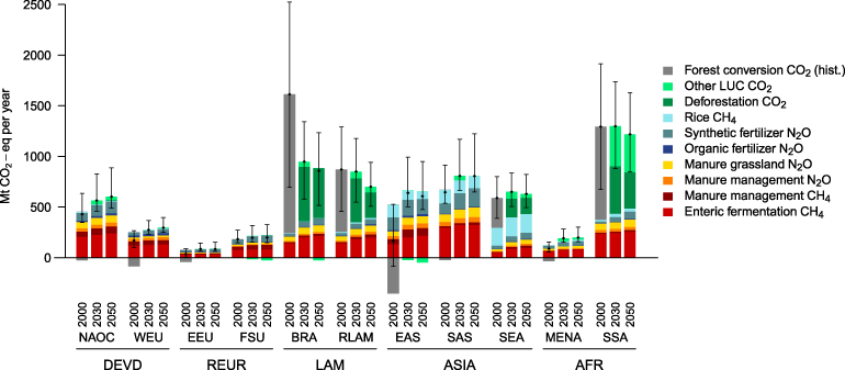
Figure 2. GHG emissions along the baseline for different regions and sources. All calculations are produced with the model, except for the historical emissions from forest conversion in gray, which are sourced from FAOSTAT (2000–2005 average). Error bars indicate 95% confidence intervals for total over all emissions sources (see SI available at stacks.iop.org/ERL/8/035019/mmedia). Regional groups are the same as in figure 1. Sub-regional breakdown: NAOC= North America and Oceania; WEU= Western Europe; EEU= Eastern Europe; FSU= Former Soviet Union; BRA: Brazil; RLAM= Rest of South and Central America; EAS= Eastern Asia; SAS= South Asia; SEA: South-East Asia; MENA= North Africa and Middle East; SSA= Sub-Saharan Africa.
Download figure:
Standard image High-resolution imageFollowing a different scenario of agricultural productivity can, however, significantly change the balance of future GHG emissions. In figure 3, the left panel shows how different regions react to the yield scenarios around the baseline under the 'High-Input' pathway. The right panel illustrates how the world total is modified when the pathway is changed. Under the 'High-Input' pathway, increasing yield allows emissions to be substantially decreased (−456 MtCO2-eq for 'CONV'), whereas a yield slow-down would lead to additional GHGs (+340 MtCO2-eq). The magnitude of change around the initial baseline, however, appears to be relatively limited (−7% for 'CONV'/+5% for 'SLOW') when compared with the magnitude of yield deviation. The effect of livestock feed efficiency alone appears to be slightly less efficient when compared to 'CONV' (−371 MtCO2-eq in 'CONV-L'), whereas crop yield change contribution appears to be very limited (−67 MtCO2-eq in 'CONV-C').
Different effects are indeed involved in the interplay of emission changes and can explain the observed patterns. First, yield growth obviously affects the emission factors of some sectors directly. For crops, immersed areas used for rice cultivation decrease as yield increases. However, in the case of the 'High-Input' pathway, this effect does not occur for fertilizer emissions, because the use of this input is increased to obtain greater yield. In the case of livestock, we also observe that, in most regions, livestock CH4 and N2O emissions decrease in 'CONV', because fewer animals are necessary per unit of output, and, symmetrically, they increase in 'SLOW'.
A second channel of emissions comes from the interaction of crop and livestock sectors with land use. Higher crop yield and improved feed conversion are expected to drive cropland and grassland sparing and decrease other land conversion, in particular deforestation. This is notably illustrated in the 'CONV' and 'CONV-L' scenarios in Latin America, as livestock pressure in this region is recognized as being a significant driver of deforestation. However, this effect is not observed in all cases. In the 'CONV-C' scenario, potential land savings for crops seem to be unexploited for the same region. This is explained by a third driver of emission changes: the rebound effect.
Indeed, the third factor affecting emissions comes from the demand response to prices when larger quantities are available on the market. As a result, a clear rebound effect is observed in several regions, canceling out some of the benefits from previous effects. In the 'CONV-C' scenario, livestock numbers increase by 2% as a result of more abundant feed and additional demand for cheaper ruminant and non-ruminant meat, driving one-third of extra agricultural emissions. Fertilizer emissions represent the rest of this increase, although their intensity per unit of output is assumed to decrease (elasticity of 0.75 for the 'High-Input' pathway). For regions such as Asia, this even contributes to a net increase in emissions under both the 'CONV' and 'CONV-C' scenarios. The overall magnitude of such rebound effects is in fact considerable, as we will see in section 4.3. This emphasizes the need for more careful attention to be paid to the ambiguous impact of yield increase through this channel [16].
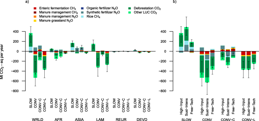
Figure 3. Differences in GHG emissions levels by 2050 across yield scenarios and regions (a) and productivity pathways by scenario at world level (b) with respect to the baseline ('TREND'). Error bars indicate 95% confidence intervals for the total of our emissions sources (see SI available at stacks.iop.org/ERL/8/035019/mmedia). Region definition: DEVD =North America, Oceania and Western Europe; REUR =Eastern Europe and Former USSR; ASIA =South-East, East Asia; LAM =Latin America; WRLD = World. Land use change annual emissions are calculated as an average over the simulation period.
Download figure:
Standard image High-resolution imageAs we have seen, the combination of these three effects plays differently across regions and scenarios. The way in which technology can be implemented is, however, another determining factor in these results. For example, total emission savings under the 'CONV-C' scenario are more than tripled when switching from high-input management to sustainable intensification (from −67 to −239 MtCO2-eq). In contrast, under the 'Free-Tech' pathway, the rebound effect appears to be even more important and agricultural emission savings are almost canceled out in 'CONV-C' (−39 MtCO2-eq) and decreased by 29% in 'CONV'. Overall, total savings vary from a ratio of 1–2 in the 'CONV' scenario depending on the way in which technology is implemented. However, total abatement always remains below the 10% magnitude.
4.2. Trade-offs and synergies between GHG mitigation and food availability
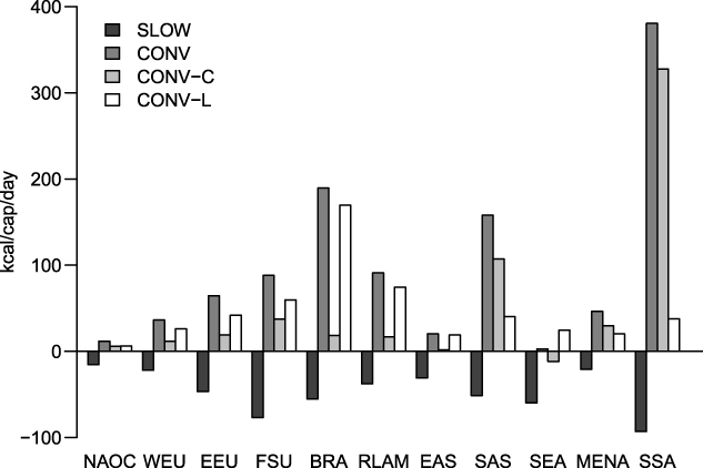
We now balance the environmental performance of yield scenarios and productivity pathways with their implications for food provision. The most direct effect of yield improvement is an increase in available calories, which reduces the price of crops and livestock for final consumers. We can therefore observe in figure 4 that the response of food demand is in the same direction as productivity change, here in the case of the 'High-Input' pathway. On average, the world consumption increase is higher by 144, 102, and 37 kcal per capita per day in the 'CONV', 'CONV-C' and 'CONV-L' scenarios, respectively, and lower by 52 kcal/cap/day for the 'SLOW' scenario. Patterns appear to differ across scenarios and regions. Demand is more elastic in less advanced regions and developing countries therefore tend to react much more than developed ones. Sub-Saharan Africa and South Asia benefit the most from closing the crop yield gap, as they are far from their potentials and have a larger share of vegetal calories in their diet. On the livestock side, Brazil and Rest of Latin America increase demand for ruminant meat and milk when feed efficiency is improved. This therefore leads to different diet compositions across scenarios, livestock products representing 16.9% of world consumption in 'CONV-C' versus 18.2% in 'CONV-L' by 2050. We find similar results for the 'Sust-Intens' pathway as we assume the same production costs in this scenario as for 'High-Input'. When comparing with 'Free-Tech', the rebound effect is however much larger with increase in consumption, by 287, 252, and 35 kcal/cap/day for the 'CONV', 'CONV-C' and 'CONV-L' scenarios, respectively, and −145 kcal/cap/day for the 'SLOW' scenario, compared with 'TREND'.
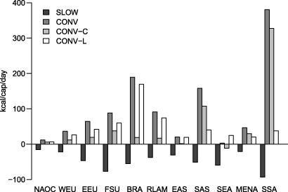
Figure 4. Change in domestic food demand (kcal/cap/day) in 2050 for the different yield scenarios and the 'High-Input' pathway.
Download figure:
Standard image High-resolution imageHow do these changes compare with the environmental gains for developing regions? Interestingly, the situation appears to contrast across scenarios and depends on the nature of productivity changes. Figure 5 presents an overview of GHG emissions (x-axis) and consumption changes (y-axis) at the world level for the different scenarios and pathways. Most points are located in the quadrants (B) and (C) of the graph, illustrating the strong synergies between food supply and GHG savings. The 'SLOW' scenario clearly appears negative for the two environmental and food dimensions, especially when land use emissions are accounted for (C). In contrast, the 'CONV' scenario is beneficial for both dimensions, with greater effects for the environment under the 'Sust-Intens' pathway, and better food supply performance under 'Free-Tech'. However, as illustrated previously, GHG emissions in agriculture tend to increase if crop yields alone are boosted through the 'High-Input' pathways and total savings are in that case limited. When fertilizer effects are removed under 'Sust-Intens', 'CONV-C' gains are much larger (blue triangles). Under the 'Free-Tech' scenario, however, the rebound effect cancels out 84% of the savings (blue squares), which illustrates well the trade-offs between mitigation and food provision through the price channel. These results contrast with the outcome from yield change in the livestock sector which allows large savings of GHG emissions with, however, limited benefit in terms of food availability. Overall, only the combination of the two productivity increases appears to be an efficient mix to obtain both food security and environmental benefits.

Figure 5. Difference in GHG emissions (x-axis) and food availability (y-axis) in 2050 for the different scenarios with respect to 'TREND'. Panels (A)–(C) and (D) delineate domains where food provision increases ((A), (B)) or decreases ((C), (D)) and GHG emission savings increase ((B), (D)) or decrease ((A), (C)). Colors correspond to the four scenarios, and the symbols at the corners of the triangle to the three productivity pathways. For the 'CONV-L' scenario, the 'Sust-Intens' and 'High-Input' pathways are similar by construction. Solid lines indicate full agriculture and land use emission accounting, and dashed lines agricultural emissions only. Land use change annual emissions are calculated as an average over the simulation period.
Download figure:
Standard image High-resolution image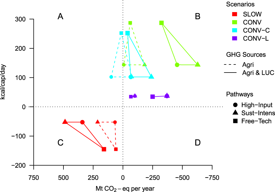
4.3. Sensitivity analysis
So far in our analysis, uncertainty has only been approached through confidence intervals on GHG emission factor values. However, some model settings or scenario assumptions also significantly influence the simulation outcomes. We summarize in table 4 the results of sensitivity analyses on four parameters: yield trend for developed regions (1); fertilizer to yield elasticity (2)–(3); price elasticity of demand (4)–(6); and carbon accounted for forest (7). The sensitivity analysis confirms that the most critical parameters are demand elasticities. In particular, removing all rebound effect leads to about a doubling of GHG emission savings. Fertilizer to yield elasticity is important for the outcome of intensification when considering agricultural emissions alone, but nitrous oxide emissions are always compensated by land use change CO2 savings. Yield growth assumptions for developed countries play only a secondary role for our findings.
Table 4. Sensitivity analysis on the difference between the CONV and TREND scenarios for GHG emissions and consumption at world level by 2050. Abbreviations: HI ='High-Input'; SI ='Sust-Intens'; FT ='Free-Tech'; LUC = land use change.
| No. | Name | TREND | CONV–TREND | ||||||||
|---|---|---|---|---|---|---|---|---|---|---|---|
| Agri 2050 | LUC Avg/yr | Agri | Agri + LUC | Conso | |||||||
| HI | HI | HI | SI | FT | HI | SI | FT | HI/SI | FT | ||
| 0 | Central scenario | 4508 | 1895 | −7 | −182 | −62 | −456 | −628 | −325 | 144 | 287 |
| 1 | Yield slow-down in developed countries (50% linear trend) | 4526 | 1950 | 8 | −169 | −40 | −411 | −587 | −310 | 137 | 285 |
| 2 | Less fertilizer needs (elasticity fertilizer to yield: 0.5) | 4408 | 1895 | −53 | −170 | −52 | −502 | −616 | −315 | 144 | 287 |
| 3 | More fertilizer needs (elasticity fertilizer to yield: 1) | 4608 | 1895 | 38 | −195 | −72 | −410 | −641 | −334 | 144 | 287 |
| 4 | More rebound effect (demand elasticities × 1.5) | 4443 | 1743 | 40 | −143 | 14 | −307 | −491 | −86 | 183 | 407 |
| 5 | Less rebound effect (demand elasticities × 0.5) | 4626 | 2231 | −75 | −238 | −157 | −704 | −869 | −688 | 92 | 156 |
| 6 | No rebound effecta (fully inelastic demand) | 4508 | 1895 | −441 | −590 | −541 | −1470 | −1617 | −1587 | 0 | 0 |
| 7 | More land use emissions (dead biomass and soil organic carbon accounted) | 4508 | 3402 | −7 | −182 | −62 | −854 | −1023 | −543 | 144 | 287 |
aTo ensure better comparability, this scenario is run on the same baseline as TREND.
5. Discussion and conclusions
The role of agricultural productivity as a potential source of mitigation has already been underlined by several studies [5, 10, 31, 6]. However, none of these used an integrated framework to concurrently analyze the contributions of different sectors and contrast the total mitigation effect related to crop, livestock, and land use change emissions together with food provision impacts.
Our results, in particular, allow three important aspects to be stressed. First, mitigation potentials from yield increase are very different for crops and for livestock. Many authors focus on crop cultivation impact alone [5, 10]; however, livestock is recognized as the main emitter of GHGs and the sector with the largest impact on land use [32, 33]. Omitting livestock from yield trends analysis can lead to a significant part of agricultural mitigation potential being overlooked. This mitigation would be even greater if the potential effects of lower crop prices on livestock system intensification and associated pasture sparing are taken into account [6]. However, the overall magnitude of the land use change savings still needs to be refined: some of our emissions are the result of complex dynamics, the extent of which could be influenced by proactive land policies, some of which have already been initiated in some regions [34]. Nevertheless, our conclusions still stand if non-CO2 gases alone are considered, as illustrated in figure 5.
Second, we have illustrated the importance of the rebound effect using an economic equilibrium model. Although this effect is not captured well by pure biophysical analyses, it does have critical importance. The results to this extent are dependent on the values of our price elasticities. Our sensitivity analysis shows that with elasticities two times lower, the rebound effect would be smaller and the mitigation would be increased by 54% (table 4, row 5). Further, without any rebound at all, mitigation of up to 1.5 GtCO2 would have been reached (table 4, row 6). The environmental implications of these rebound effects should be more systematically considered when associating food security virtues with productivity policies, as they are intrinsically linked to the increase of production for more food provision.
Last, we have shown that different productivity pathways would have different implications. In particular, the combined effect of rebound and fertilizer increase would not allow for GHG emission savings when crop yields alone are increased (CONV-C under 'High-Input'). More importantly, the implications of productivity gains for producer prices are fundamental to anticipating the magnitude of the rebound and the environmental benefits. Pathways relying on total factor productivity gains like 'Free-Tech', by reducing producer costs, maximize production but limit environmental benefits. The literature indicates that TFP played a greater role in recent production development [35] and that this trend should continue [36]. Therefore, complementary measures may be needed on the consumer side to counter-balance this effect. For example, the efficiency of a diet shift to less meat has been demonstrated [37, 38]. More general combination of supply and demand side measures appears desirable but also faces some reality constraints, as change of consumer demand is subject to more inertia [4]. The gains from investment towards agricultural productivity gains would allow more immediate GHG savings, but a combination of efforts in the crop and livestock sectors appears as the most efficient way to create synergies on both the food supply and mitigation sides.
Acknowledgments
This research was supported by the EU-funded FP7 projects ANIMALCHANGE (grant no. 266018) and FOODSECURE (grant no. 290693). The authors would like to thank three anonymous reviewers for their valuable comments that contributed to the improvement of this article.
Footnotes
- 5
The land use change estimate in our baseline is lower than the historical deforestation emission rate in certain regions because (i) the model does not account for some drivers of deforestation such as illegal logging, infrastructure expansion, and mining activities, (ii) some policy shifts are reflected, such as the better protection of forest recently observed in Brazil, (iii) the baseline follows a productivity trend for crop and livestock that relieves part of the pressure on land (see SI for more details on land use change emissions.)