
Abstract
Here, we assess current stress in the freshwater system based on the best available data in order to understand possible risks and vulnerabilities to regional water resources and the sectors dependent on freshwater. We present watershed-scale measures of surface water supply stress for the coterminous United States (US) using the water supply stress index (WaSSI) model which considers regional trends in both water supply and demand. A snapshot of contemporary annual water demand is compared against different water supply regimes, including current average supplies, current extreme-year supplies, and projected future average surface water flows under a changing climate. In addition, we investigate the contributions of different water demand sectors to current water stress. On average, water supplies are stressed, meaning that demands for water outstrip natural supplies in over 9% of the 2103 watersheds examined. These watersheds rely on reservoir storage, conveyance systems, and groundwater to meet current water demands. Overall, agriculture is the major demand-side driver of water stress in the US, whereas municipal stress is isolated to southern California. Water stress introduced by cooling water demands for power plants is punctuated across the US, indicating that a single power plant has the potential to stress water supplies at the watershed scale. On the supply side, watersheds in the western US are particularly sensitive to low flow events and projected long-term shifts in flow driven by climate change. The WaSSI results imply that not only are water resources in the southwest in particular at risk, but that there are also potential vulnerabilities to specific sectors, even in the 'water-rich' southeast.
Export citation and abstract BibTeX RIS

Content from this work may be used under the terms of the Creative Commons Attribution 3.0 licence. Any further distribution of this work must maintain attribution to the author(s) and the title of the work, journal citation and DOI.
1. Introduction
Water availability in the United States (US) is a function of relative supply and demand. According to the most recent estimates (2005) of US water withdrawals, freshwater demands are driven by agriculture (37%), thermoelectric power generation (41%), and municipal requirements (19%) (Kenny et al 2009). Despite a growing US population (Mackun and Wilson 2011), total water use, defined as both withdrawals and consumption, by the agricultural and municipal sectors has remained relatively unchanged since 1985 (Kenny et al 2009) reflecting declines in per capita usage by these sectors. Total water withdrawals for electricity generation have remained consistent, only 3% growth between 1995 and 2000 (Kenny et al 2009), although a modest 6% increase in consumptive use occurred between 1990 and 1995 (Solley et al 1998).
Despite stabilization of recent water demands, there is significant uncertainty in how future water demands may evolve. This uncertainty stems from the impacts of economic factors (e.g., Qi and Chang 2011), social behaviors (e.g., Gleick 2003), technological innovations (e.g. Jury and Vaux 2005), legal and policy drivers (e.g., Adler 2009), demand hardening (e.g., Howe and Goemans 2007), and climate change (e.g., Brown et al 2013). For example, a national transition from once-through to recirculating cooling processes at thermoelectric power plants is projected to increase water consumption by the electricity sector by as much as 165% by 2025 (Hoffman et al 2004).
On the water supply side, surface and ground water resources have been declining in much of the US (Karl et al 2009). Aquifers underlying the Central Valley in California and the Ogallala, which spans the area between Nebraska and Texas, are being drawn down more rapidly than they are being recharged (Scanlon et al 2012, Taylor et al 2013). Approximately 23% of annual freshwater demands rely on groundwater resources (Kenny et al 2009), yet the volume of groundwater remaining is unclear (Reilly et al 2008, Taylor et al 2013).
Average surface water supplies are decreasing, and are expected to continue declining, particularly in the southwestern US (Udall 2013, Hoerling et al 2013). Also in the southwest, water availability is defined as much by legal regimes as by physical processes. Water rights define how much and when water may be withdrawn from surface water sources irrespective of how much water may or may not be flowing in a given year. Water quality, including temperature and sediment concentration, can also constrain availability for certain users.
Although national trends point towards relatively stable demands as increases in efficiency are offsetting increases in population, declines in supplies may be sufficient to introduce vulnerabilities to sectors dependent on water resources. Future projections of water supplies and demands vary regionally and locally, but it is clear that climate change stands to increase national water demands and diminish national water supplies (Foti et al 2012, Brown et al 2013).
To understand possible risks and vulnerabilities to regional water resources and the sectors dependent on freshwater, we assess current stress in the freshwater system based on the best available data. We present spatially explicit measures of freshwater supply stress for the coterminous US, defining water stress as the ratio of water demands to water supplies. We present a basin-scale analysis as the national averages mask significant regional deviations from supply and demand trends. We focus on a snapshot of contemporary annual demands and compare these against different water supply regimes, including current average supplies, current extreme-year supplies, and projected future average supplies under climate change. In addition, we investigate the sectoral contributions to current water stress and the relationship between water stress within a basin related to water withdrawals and that related to water consumption.
2. Methods
For this analysis, water stress is expressed as a ratio of water demands to water supplies for each individual watershed basin, where watersheds are defined at the 8-digit Hydrologic Unit Code (HUC) scale (USGS 2012). The USGS continually refines the HUC boundaries. Here, we use the 2009 Watershed Boundary Dataset provided by Natural Resources Conservation Service (NRCS 2009).
We calculated water supply stress following a modified version of the water supply stress index (WaSSI) (Sun et al 2008, 2011a, Caldwell et al 2011, Tavernia et al 2012) as in equation (1). The WaSSI for each watershed i was calculated as the ratio of annual water demands to annual water supplies for that watershed, as in:

where WDi is watershed i's annual demand for water withdrawals, SWi is watershed i's annual surface water flows including those from upstream watersheds, and GWi is watershed i's annual volume of groundwater available for water supply. Equation (1) represents water stress only with respect to water withdrawals; it measures whether water supplies are sufficient for all withdrawal requirements within a watershed to be met concurrently. The WaSSI was calculated separately for water withdrawals and for water consumption, where the latter metric incorporates return flows in the indicator's numerator. With few exceptions, watersheds follow similar trends (data not shown). For this reason, the WaSSI for water withdrawals is used in this analysis and throughout the discussion.
Water supply stress was also calculated for each major sector (agriculture, municipal, thermoelectric) at the watershed scale. The water supply stress due to an individual water use sector s (WDi,s) was calculated as:

The greater the WaSSI value, the greater the water supply stress. Two important assumptions in our calculation of WaSSI are that water is being supplied by local natural sources and that groundwater supplies are unlimited, i.e., that groundwater withdrawals will continue at present rates despite whatever overdrafts and impacts are thusly implied. Although groundwater stores are declining in many places because of withdrawals, there are limitations on the quality of data about remaining volumes and drawdown rates (Reilly et al 2008). Given that there is also no national dataset available with the appropriate information at the scale necessary for this analysis, the only options are to either assume ground water is infinitely available or completely unavailable. We chose to assume the former as is consistent with other analyses of water stress (e.g. Roy et al 2012).
A given basin's water stress, signified by a WaSSI greater than 1.0, may be overestimated because demands are being met by built infrastructure (e.g. reservoirs, interbasin transfers), or by additional water sources (e.g. enhanced groundwater pumping; reclaimed or recycled water). The large differences in the amount of precipitation between eastern and western US generally results in chronically higher stress index for western states. For example, a stress index of 0.30 would present normal stress conditions in the west, while the same value would represent extreme water stress in the east. In addition, water quality constraints are not considered in the analysis, and the potential impacts of water withdrawals on surface water supplies in downstream basins are also omitted. Though beyond the scope of this analysis, these issues are important considerations for understanding the complete picture of water resources.
2.1. Water supplies
Annual surface water supply (SWi) over the period 1999–2007 was estimated for each watershed by the WaSSI (Sun et al 2008, 2011a, Caldwell et al 2011, 2012). On a monthly timescale, this model simulates the full water balance for each 8-digit HUC watershed in the coterminous US using spatially explicit data, including MODIS land cover and soil information. This modeled water balance accounts for precipitation, snow accumulation and melt, rain infiltration, evapotranspiration, runoff and baseflow processes, as well as inflow and outflow for each watershed. Evapotranspiration is estimated based on multisite eddy covariance measurements (Sun et al 2011a, 2011b) and infiltration, soil storage, and runoff processes are estimated based on algorithms from the Sacramento Soil Moisture Accounting Model and STATSGO-based soil parameters (Koren et al 2003). A conservative flow routing model representing the stream network connects the inflow and outflow among watersheds.
Using average surface water supplies smooths idiosyncratic temporal variability and provides an appropriate baseline for estimating average future water supplies. To assess the sensitivity of the WaSSI calculation to changes in surface supplies, we also calculated the lowest annual surface flows and highest annual surface flows from the period of 1999–2007 for each individual watershed i.
The contribution of groundwater to water supplies in watershed i (GWi) were based on 2005 rates of groundwater withdrawals reported by the USGS (Kenny et al 2009). These data were resampled from the county scale to the 8-digit HUC level.
To estimate future water supplies, we held groundwater withdrawals constant at present rates and scale runoff by the projected percentage changes in average annual runoff from a baseline climate for 1900–1970 to that projected for 2041–2060 using the A1B SRES scenario (Milly et al 2005).5 We spatially interpolated the Milly et al. data from a grid (approximately two degrees longitude by two degrees latitude scale) onto the 8-digit HUC scale by matching the nearest grid centers to each watershed, then propagate these changes through the flow routing network as above. These change estimates provide a well-established, spatially explicit approximation of changes in surface freshwater supplies consistent with the central predictions of a large number of general circulation models.
2.2. Water demands
We estimated water demands separately for agriculture, municipal uses, and thermoelectric cooling, with the first two based on Kenny et al (2009) and the last on the approach of Averyt et al (2013). Kenny et al (2009) report 2005 data on water withdrawals for each of the following water uses: public supply, domestic, irrigation, livestock, aquaculture, industrial, mining, and thermoelectric power. For sectoral analysis, we combine these into three main water use sectors: thermoelectric cooling, agricultural (including irrigation and livestock), and municipal (including public supply, domestic, and industrial).
Evidence suggests numerous limitations and uncertainties in the federally reported thermoelectric water data (GAO 2012, Averyt et al 2013). For this reason, water use by the thermoelectric sector was estimated based on a combination of data reported to the Energy Information Administration (EIA) on forms 860 and 923 (EIA 2008a, 2008b) and generation-technology specific water use factors (Macknick et al 2012), as described in more detail in Averyt et al (2013). As shown in table 1, the central estimate from these data conforms closely to the commonly used estimates from Kenny et al (2009). Analysis herein relies on the central estimate. (See Meldrum et al (2013) for sensitivity analysis of the range of estimates.)
Table 1. US thermoelectric power plant water withdrawals as percentage of US total water use.
| 2007 data from Averyt et al (2013) | 2005 data reported by USGSb | |||
|---|---|---|---|---|
| Central estimatea | Minimum estimatea | Maximum estimatea | ||
| Withdrawal (%) | 36 | 22 | 45 | 41 |
| Consumption (%) | 3 | 2 | 4 | 3 |
aCentral, minimum, and maximum refer to the range of water use coefficients from Macknick et al (2012); see Averyt et al (2013) for discussion. bWithdrawal estimate from Kenny et al (2009).
3. Results
The results show 9.2% (193 of 2103) of the HUC-8 watersheds have a WaSSI greater than 1.0, meaning that demands for freshwater sources outstrip natural supplies (figure 1). According to the WaSSI, most of the water stress in the United States is indicated in the west, where there are fewer surface water resources compared with the east. There are also indications of stress in the watersheds around the Great Lakes, along the Mississippi River, and sporadically along the Appalachian Mountains. To meet demands, the western regions in particular rely on reservoirs with multi-year storage capacity to store snowmelt, as well as conveyance systems to bring water from other basins.
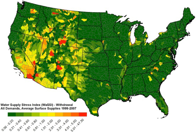
Figure 1. Withdrawal water supply stress index (WaSSI) for all demands and average water supplies, 1999–2007.
Download figure:
Standard image High-resolution image3.1. Water supply stress by sector
National average water demand statistics mask what are highly regionalized, sector-specific trends. Understanding the spatial distribution of water withdrawals by sector is important for assessing the scope of vulnerabilities. Figures 2, 3 and 4 show the spatial differences among the relative contributions of agriculture, municipalities, and power plants, respectively, to total water demands and to water stress (WaSSI).
WaSSI values >1 are shown when withdrawn water exceeds naturally available surface water and recent groundwater withdrawal rates. Thus, WaSSI > reflects either limitations on additional demands for water resources, or reliance on alternative water supplies to meet demands. For example, in some places water availability may limit growth in the agriculture sector. On the other hand, in some locations water may come from alternative sources (e.g. groundwater overdraft, reclaimed water, imported water) to meet demands.
Irrigated agriculture dominates water withdrawals along the lower Mississippi River Basin and the majority of the western United States, with the main exceptions being major population centers and directly on the Pacific Coast (figure 2(a)). Agricultural demands, by themselves, result in stress (WaSSIagricultural > 1) in 6.1% of the HUC-8 watersheds in the entire US, and 10.3% (128 of 1239) in the western US (figure 2(b)). It is well documented that irrigated agriculture is a significant contributor to the depletion of the Ogallala Aquifer and the groundwater resources in central California (Siebert et al 2010, Scanlon et al 2012, Taylor et al 2013). The WaSSI analysis assumes that there is no limit on groundwater supplies, thus the extent of stress associated with agricultural water withdrawals is not entirely reflected in figure 2(b).
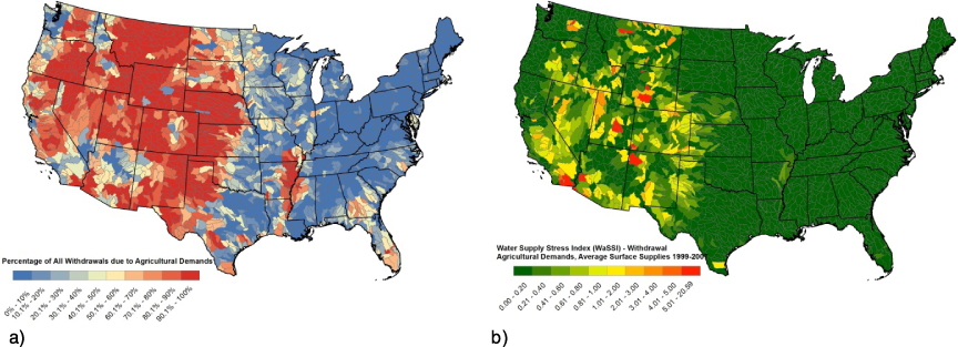
Figure 2. The agricultural contribution to WaSSI for average supplies 1999–2007. (a) shows the percentage of total withdrawal demands by agriculture for each HUC-8 watershed; (b) is WaSSI based only on agricultural demands.
Download figure:
Standard image High-resolution imageThe trend in withdrawals to support municipal demands is centered around major population centers, including southern California across to central Arizona, the Seattle–Portland corridor, and through the expanse from Texas towards New England (figure 3(a)). This is not surprising given that the majority of the US population and the majority of US industrial centers are located east of the Mississippi River. However, only in southern California, southern Nevada, the Front Range of Colorado, New Mexico, and the Great Lakes region, do municipal demands, by themselves, result in stress (WaSSImunicipal > 1) (figure 3(b)).
The expanse of municipal stress indicated across southern California and southern Nevada reflects how demands in the region are met by imported water from both north California across the Tehachapi Pass via the California Aquaduct, and from the Colorado River. Because of the links across basins, the broad picture of water stress in this region not only includes municipal demands outpacing local supplies, but also conditions in distant watersheds, including hydrology, as well as changing socio-economic, political, legal or physical infrastructure conditions that might affect these alternative water sources.

Figure 3. The municipal contribution to WaSSI for average supplies 1999–2007. (a) shows the percentage of total withdrawal demands for municipal uses for each HUC-8 watershed; (b) is WaSSI based only municipal demands.
Download figure:
Standard image High-resolution imageAlthough predominant in the eastern US, the pattern of water demands by thermoelectric power plants displays less homogeneity than the other sectors analyzed (figure 4(a)). Thermoelectric power plants withdraw more water at the point scale compared with an individual farm or town. The domination of agricultural and municipal water withdrawals across large swaths of adjacent watersheds is an aggregation of many users who are mutually dependent on natural and urban resources, respectively. In contrast, it is clear in figure 4(b) that a single power plant can create water stress in a watershed, assuming no return flows. There are 23 HUC-8 regions in figure 4(b) that show a WaSSI greater than 1.0. Within these watersheds, there are 68 thermoelectric power plants that require cooling (generating 390 TWh/year). According to WaSSI, the water stress posed by thermoelectric water demands is minimal from a national perspective6. Yet, at the local scale, it is clear that water supply stress can emerge rapidly in a watershed with the introduction of one power plant.

Figure 4. The thermoelectric contribution to WaSSI for average supplies 1999–2007. (a) shows the percentage of total withdrawal demands by thermoelectric power plants for each HUC-8 watershed; (b) is WaSSI based only thermoelectric demands.
Download figure:
Standard image High-resolution image3.2. Water supply stress: surface supply sensitivity
The analyses above incorporated a baseline surface water supply averaged over the period 1999–2007. However, surface water supplies are highly variable over short time scales, and the WaSSI is sensitive to any change in surface water supply estimates. The sensitivity analysis in figure 5, based on extreme annual flows observed over the analyzed time period, shows how changes in annual surface water supplies shift the WaSSI indicator. It is clear that flows averaged over even a modest period of time such as that used in this study may not adequately characterize watershed-scale supply stress and associated vulnerabilities.
The data in figure 5 are not intended to represent the entire scope of possible extreme WaSSI scenarios. A more sophisticated analysis of water supply records by watershed would be necessary to generate a risk profile. However, the analysis provides some general insights about regional trends in water use.
For example, during the lowest surface water flows recorded between 1999 and 2007 for each HUC-8 region (figure 6), water stress increased in nearly all watersheds (2100 out of 2103) versus water stress based on average flows. However, average increases (both in terms of raw WaSSI and in percentage changes) are much more pronounced in the western US (average WaSSI increase of 1.26, or 261% greater, by watershed) than in the east (average WaSSI increase of 0.10, or 104% greater, by watershed) (figure 5(a)). The dramatic shift in the west corresponds to a greater interannual variability in surface water supplies relative to the east. Therefore, WaSSI based on averaged flows masks the relatively larger interannual variations in the western US. When the highest flows were used to calculate WaSSI (figure 5(b)), 4.3% (90) of watersheds still showed some degree of stress (WaSSI > 1.0), most of which were in the West (79, or 6.4% of 1239). These regions must be dependent on imported and stored water to meet demands.

Figure 5. Withdrawal water supply stress index (WaSSI) sensitivity to low (L) and high (R) annual surface water supplies, 1999–2007. For each HUC-8 the lowest (a) and highest (b) annual flow occurring between 1999 and 2007 was selected and used to calculate WaSSI. This is not intended to represent large-scale spatial evolution of a low or high flow event, but to illustrate the sensitivity of WaSSI to surface supplies in different regions.
Download figure:
Standard image High-resolution image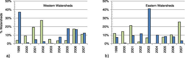
Figure 6. Percentage of watersheds for which estimated annual surface flows are the minimum (green) or maximum (blue) over the period 1999–2007 in the western (a) and eastern (b) United States. East is defined by 2-digit HUCs 01–09, west by 10–18. Both drought and flood events punctuated the baseline period used to represent average surface flows in figure 1 (1999–2007). As reflected by the years of high and low flows for each basin shown in figure 5, a widespread drought event occurred in 2002 in the west, while 1999 was a particularly wet year in the region. In the east, high surface flows occurred during 2003, while 2007 saw significant drought and associated low flows.
Download figure:
Standard image High-resolution image3.3. Water supply stress: climate change
Climate change will impact the hydrologic cycle and affect sectors dependent on water resources (e.g. Karl et al 2009) Projected shifts in the water cycle and surface water availability are not uniform across the United States. For example, total surface water supplies in the Pacific Northwest are projected to increase, while in the southwest, declines in runoff of approximately 10% are expected (Seager et al 2012).
Figure 7 shows the effects of projected climate-driven changes in US surface water flows (based on Milly et al 2005) on current water stress (shown in figure 1). It is clear that the effects of climate change on water stress will manifest differently from watershed to watershed. In most watersheds east of the Mississippi River and in select parts of the northern half of the US, projected increases in surface water flows relieve water stress by up to 10%. In contrast, throughout the rest of the US, declines in surface flows could exacerbate water stress by 15–30%. Watersheds in California, Nevada, Utah, Arizona and New Mexico show the most dramatic increase in WaSSI. Even in areas where local runoff is projected to increase, dependency on streamflows from areas with decreased runoff can create higher projected WaSSI, as can be observed along major rivers in the middle of the country. The scenario presented in figure 7 does not portray an actual, predicted future. Rather, it is an indicator of how a shift in a single dimension (surface water) can affect water stress.
The entire scope of how climate change may alter water stress is not represented in the WaSSI analysis shown in figure 7. This analysis does not include how climate change may impact groundwater supplies or alter demand regimes (Brown et al 2013), as projected shifts in these demands are highly uncertain. Although many evaluations of future water stress project changes in both water supplies and water demands concurrently (e.g. Roy et al 2012, Vorosmarty et al 2000), we hold present-day water demands constant. Uncertainty in the trends of future water demands differs from that of future water supplies. Accordingly, we isolate the effects of projected climate-driven changes in surface water supplies (Milly et al 2005) on water stress. As such, this quantitative analysis provides a transparent baseline for discussing how expected climate-driven changes in surface water might affect water stress of different sectors under a variety of possible changes in trends in water demands.

Figure 7. Percentage change in withdrawal WaSSI under climate-driven changes in surface water flows (Milly et al 2005) compared with figure 1.
Download figure:
Standard image High-resolution image
4. Discussion
The WaSSI model is best used as a tool to identify regions with potential vulnerabilities to prompt additional research geared towards understanding the complexity of issues affecting water supplies and demands. The analysis presented here is not intended to represent an explicit future possibility. Rather, the components contributing to water stress are teased apart in order to show the relative spatial vulnerabilities to specific sectoral demands alongside changes in surface water supplies.
Demand- and supply-side factors contributing to water stress are highly regionalized. Surface water stress is predominant throughout the western half of the US, where natural surface water supplies are insufficient to meet demands in many watersheds (figure 1). In regions where the WaSSI > 1.0 under current supply and demand regimes, surface water supplies are supplemented by built infrastructure (i.e., reservoirs and conveyance) and groundwater.
Vulnerabilities to sectors dependent on water resources are not isolated to impacts to local watershed supplies. Risks also stem from impacts to water resources in distant regions, as well as from impacts to the reliability of built infrastructure and associated management regimes. Southern California is an example of where demands are not being met by local water supplies (WaSSI > 1.0, figure 1). The region depends extensively on bringing water in from both the Colorado River and northern California to enhance supply. Therefore, although water demands are generally being met, the WaSSI analysis suggests that the region may be at risk should water supplies from the Colorado River and northern California diminish, or should the infrastructure that stores and conveys water to California falter.
One important caveat related to WaSSI is that it does not account for the volume of groundwater remaining; the analysis assumes unlimited groundwater supplies. For example, the entire region overlying the Ogallala Aquifer shows no current water stress, yet the aquifer is being overdrawn and current water withdrawals are not sustainable (e.g. Scanlon et al 2012). Specific analysis of the role of groundwater is beyond the scope of this analysis, but will be the target of future investigations.
Spatial patterns of water stress vary substantially across different water use sectors. Agriculture is the major demand-side driver of water stress across the majority of the US, while extreme municipal stress is concentrated in the greater Los Angeles and Las Vegas areas. Water stress introduced by cooling water demands for power plants is punctuated across the US, indicating that a single power plant has the potential to stress surface supplies, especially in local areas. Given the potential for growth in the electricity sector, the portfolio of water demands and supplies in a watershed and cooling system design options should be considered when siting power plants.
The sensitivity of water stress to surface water supplies is useful for evaluating risks posed to different demand sectors under different scenarios. It can also be used as a tool for assessing adaptive capacity. Consider the similarity between the degree of water stress indicated by historically low surface flows (figure 5) and projected in surface flow (figure 7) in the western states. This suggests that assessing current adaptive capacity during low surface water supplies (i.e. drought) may be a reasonable first step for evaluating the ability of current institutions to cope with average changes in surface water supply resulting from climate change. Conversely, because figure 7 reflects long-term shifts in averages whereas figure 5 depicts short-term deviations from averages, it also suggests that if interannual variability in flows remains proportionally consistent over time, WaSSI under future climate change may be even more pronounced than average-based projections imply. Although the projections in figure 7 do not convey information about changes in the nature of variability and extremes in the hydrologic system that may occur with climate change, such information can provide a useful first step in assessing vulnerability of individual sectors to climate change under current demand scenarios. In addition, because these projections are presented in isolation of other sources of uncertainty, such as trends in population or water use efficiency, they provide an important baseline for understanding the role of supply-side changes in driving future water supply stress.
Acknowledgments
We greatly appreciate the support of the Union of Concerned Scientists, The Energy and Water in a Warming World initiative (EW3) contributors, and the EW3 Scientific Advisory Committee. Additional support was provided through the NOAA Western Water Assessment and the Cooperative Institute for Research in Environmental Sciences at University of Colorado Boulder. We are grateful to two anonymous reviewers whose comments and contributions greatly improved this letter.
Footnotes
- 5
These projections come from an ensemble of 12 general circulation models that were selected for performance in modeling observed changes in twentieth century flows between the period of 1900–1970 and that of 1971–1998.
- 6
However, in cases of high WaSSI, withdrawals in a given, individual basin would be expected to have negative impacts on water supplies on downstream basins with limited additional sources of inflow, thus increasing that downstream basin's WaSSI. This potential effect is outside the scope of the present analysis.