

Abstract
Biochar may contribute to climate change mitigation at negative cost by sequestering photosynthetically fixed carbon in soil while increasing crop yields. The magnitude of biochar's potential in this regard will depend on crop yield benefits, which have not been well-characterized across different soils and biochars. Using data from 84 studies, we employ meta-analytical, missing data, and semiparametric statistical methods to explain heterogeneity in crop yield responses across different soils, biochars, and agricultural management factors, and then estimate potential changes in yield across different soil environments globally. We find that soil cation exchange capacity and organic carbon were strong predictors of yield response, with low cation exchange and low carbon associated with positive response. We also find that yield response increases over time since initial application, compared to non-biochar controls. High reported soil clay content and low soil pH were weaker predictors of higher yield response. No biochar parameters in our dataset—biochar pH, percentage carbon content, or temperature of pyrolysis—were significant predictors of yield impacts. Projecting our fitted model onto a global soil database, we find the largest potential increases in areas with highly weathered soils, such as those characterizing much of the humid tropics. Richer soils characterizing much of the world's important agricultural areas appear to be less likely to benefit from biochar.
Export citation and abstract BibTeX RIS

Content from this work may be used under the terms of the Creative Commons Attribution 3.0 licence. Any further distribution of this work must maintain attribution to the author(s) and the title of the work, journal citation and DOI.
1. Introduction
Biochar—defined as pyrolyzed (charred) biomass applied to soil—has elicited significant interest as a strategy for mitigating climate change, and as an agricultural soil amendment [1–3]. While the long-term persistence of pyrogenic organic material in soil is not well constrained, there is evidence that its residence time can be considerably greater than that of other plant-derived inputs to soil [4–6]. Production and application of biochar may thereby offer a means of drawing down atmospheric CO2 concentrations over time by stabilizing dead plant carbon that would otherwise be mineralized more rapidly [7]. Inasmuch as biochar is an effective plant fertilizer, it may offer a 'win–win' between climate change mitigation and agricultural production by sequestering carbon, improving soil fertility, and potentially reducing soil non-CO2 greenhouse gas emissions [8–10].
The upper bound for climate change mitigation through biochar systems has been estimated at approximately 12% of 2010 CO2-equivalent greenhouse gas emissions per year [2]. Of course, realized mitigation benefits are likely to be lower than this estimated technical potential, with the gap between technological potential and realized benefit depending in large part on the degree to which farmers and other land managers produce and/or apply biochar to the soils that they manage. Given that farmers and land managers are unlikely to utilize biochar in large quantities unless its use is profitable, the degree of biochar technology adoption will in turn be strongly dependent on its costs and benefits—neither of which are well understood.
Increased crop yields are an important part of this benefit. Numerous controlled field and greenhouse experiments have investigated yield response to biochar, and results have been summarized in several reviews [3, 11–14]. Quantitative reviews have estimated average yield benefits from biochar at approximately 10% for crop productivity (encompassing both harvested yields and aboveground biomass production) [11] and approximately 25% for aboveground biomass [12]. Variability of these benefits is high however, ranging between cases where biochar caused a near-failure in plant growth [15] to cases where biochar caused plants to grow where they would otherwise have failed [16, 17]. It seems clear that this variability is mediated by soil properties and properties of the applied biochars. Quantitative reviews have found yield response to be relatively higher in sandy soils, moderately acidic soils, and in response to biochar produced from animal waste [11, 12].
However, quantitative reviews have been hindered by missing and/or inconsistent reporting of soil properties, biochar properties, or other factors which may explain observed plant response. Therefore they have employed univariate meta-analyses of subsets of published data to calculate average responses in under different experimental conditions [11], or fit linear regression models using only those predictor variables that were reported in the majority of available primary studies [12]. While useful as a 'first pass' at the data, these approaches may lead to misleading and/or imprecise conclusions stemming respectively from correlation between grouping factors and underlying causes, and low effective sample sizes caused by dropping observations with missing covariate data. The former issue may increase omitted variables bias, while the latter may limit the global significance of these reviews by rendering them unable to use the full set of available studies.
This letter addresses these challenges by using statistical methods designed for problems with missing data [18], thereby allowing us to use a more complete set of available studies. First, we seek to infer how biochar's agricultural yield benefit is mediated by varying soil characteristics, biochar characteristics, and management factors. We do so by constructing a semiparametric meta-regression model [19–21] and fitting it to a dataset comprised of 365 observations from 40 studies which compared crop yields in biochar-using treatments to biochar-free controls. Second, we seek to predict where across the globe biochar is likely to have the greatest agricultural benefit. We do so by projecting our fitted model onto a global database of soil properties [22], for a representative biochar at an agriculturally plausible application rate.
2. Data and methods
2.1. Data
We extracted data on crop and/or biomass yields, biochar properties, and soil properties from 84 studies that examine effects of biochar on plant growth (citations of original studies, as well as full dataset, in SI available at stacks.iop.org/ERL/8/044049/mmedia). Studies were identified using academic search engines, and both peer-reviewed and 'gray' literature is included in our dataset. Variables from the original studies were selected for inclusion into our dataset based on consistent availability across original studies, and theoretical importance. Many key drivers of yield could not be included however, particularly soil nutrient contents. We ignore soil nitrogen, phosphorous, potassium, etc, because measures of total content correlate only imperfectly to availability given heterogeneous soil chemistry. Rather than controlling for them explicitly, we account for them indirectly by using random effects (see below).
Our dataset includes studies that reported crop yield, plant biomass production, or both. We use the full set of studies to drive imputation models for the prediction of missing data (described below). We then discard those studies that do not provide measurements of grain, legume, or aboveground non-tree fruit yield. 40 of our 84 studies report crop yields.
Absolute crop yield or plant biomass production is not readily comparable between studies because of heterogeneity in plant species. To make studies comparable, we analyzed data as response ratios [23, 24], defined as the natural logarithm of the ratio of biomass production or crop yield in a given (biochar-incorporating) treatment, to its respective zero-biochar control: RR ≡ ln(yieldtreatment÷yieldcontrol). This ratio is comparable between diverse studies, while the logarithmic transformation ensures that variability in the ratio's denominator has no greater influence on the metric than variability in its numerator. A response ratio of 0 indicates no change from the control. Response ratio is readily transformed into a percentage relative increase RI = (eRR − 1) × 100%. If a study applied biochar at multiple rates, we calculate a separate response ratio for each treatment level using a common zero-biochar control mean. We thus construct a dataset of 365 crop yield response ratios, with associated soil and biochar covariates.
Distributions of variables that we analyze, response ratios, and univariate correlations between variables, are presented in supplementary figures S1–S3 (available at stacks.iop.org/ERL/8/044049/mmedia). Our data contains a broad range of soil properties, biochar properties, and response ratios, though with some gaps and anomalies. For example, no studies in our dataset used biochar produced between 650 and 900 ° C. Furthermore, there was no strong univariate relationship between percentage carbon and pyrolysis temperature. This was somewhat unexpected, given laboratory studies showing increasing carbon content as a function of pyrolysis temperature [25], though it is possible that this simple correlation is driven by other correlated factors, such as feedstock or pyrolysis technology. Increasing pyrolysis temperature was correlated with increasing pH [26], while increasing pH was associated with lower carbon content. Based on bivariate comparisons of available data, neither the response ratio nor its variance were well-explained by any of the variables singly (figures S1–S3 available at stacks.iop.org/ERL/8/044049/mmedia), though there are suggestive correlations between response ratio and soil pH and CEC. This lack of strong univariate explanatory power was a key motivation for our use of the multivariate methods. Finally, we classify the biochars used into one of three categories; 'woody', 'nonwood', and 'manure'. 'Woody' biochars are those made from wood, 'nonwood' biochars are those made from plant matter other than wood (mainly crop residues), and 'manure' biochars include any that are derived from animal waste. 18 studies in our crop yield dataset use nonwood chars, 18 use wood chars, and eight use manure chars. For variables that we include in our analysis that were missing in primary studies, corresponding authors were contacted with requests for those data. Nevertheless, we lack observations on one or more variables from the majority of the studies in our dataset (figure S4 available at stacks.iop.org/ERL/8/044049/mmedia).
2.2. Methods
Our dataset and context have a number of distinctive features that have shaped the analytical methods that we use. First, our dataset is comprised of studies, rather than primary data. We therefore draw upon 'meta-regression' techniques [27, 28], in which observed effects are modeled as a function of a study-level random effect and a set of explanatory fixed effects. We specify random effects at the level of unique soil–biochar combination. This is a slightly lower level than study-level, and is motivated by the fact that several studies investigate several different soil–biochar combinations. It is nonetheless a higher level than a random effect at the common-control experiment level; given that there are 230 of these, with many singletons, specification of random effects at this level would adversely affect confidence intervals [29] while also over-fitting the model. Observations are weighted such that each common-control experiment in our dataset is given equal weight, i.e. such that common-control experiments applying biochar at several different application rates do not influence our estimates any more than studies examining fewer application rates. As is standard practice in meta-regression, we further weight our observations by the inverse of the variance of the response ratio—a practice aimed at addressing publication bias and up-weighting studies whose effects are more precisely estimated [27, 28]. Because our distribution of response ratio variances is highly skewed and in all cases between zero and one, we weight by the logarithm of the inverse of the variance.
Second, many of our observations contain missing data along one or more covariates of interest (figure S4 available at stacks.iop.org/ERL/8/044049/mmedia). We use multiple imputation [18, 30] to draw inference using observed data from partially missing vectors of observations. Specifically, we construct multiple imputations via chained equations (MICE) [31, 32], with a relatively large number of imputations (M = 200) chosen for numerical stability and result replicability. Details of our imputation modeling and R code for implementation are available in SI (available at stacks.iop.org/ERL/8/044049/mmedia). Briefly, the MICE algorithm operates as follows: It begins by filling in missing values with arbitrary values. It then cycles through each variable and constructs a regression model to fit the partially observed dependent variable to a partially observed and partially imputed dataset comprised of the other variables. These models are then used to update the initial arbitrary imputations, in the form of a draw from the fitted regression model's predictive distribution. We cycle through the set of variables many times until our imputations approximately converge in distribution, saving the values at the final step. We repeat this entire process once for each of the M = 200 imputations, generating 200 slightly different datasets with missing values 'filled in' with plausible guesses as to what the missing values might have been. The 200 fitted models are then combined according to Rubin's rules [18]; averaging coefficient vectors, averaging variance–covariance matrices, and adding a non-negative correction to variance–covariance matrices that is inversely proportional to the predictive ability of our imputation models. The effect is to widen confidence intervals where there is either a lot of missing data or where missing values of data are poorly predicted by observed data.
Third, we have little prior justification for assuming linear relationships between our observed variables and crop yield response ratio, nor do we have strong a priori knowledge of appropriate functional forms to use. We therefore use semiparametric techniques to estimate smooth functions mapping our independent variables to RR, employing generalized additive models [33] fit with the mgcv package in R [19, 20].
Finally, because our dependent variable is the logarithm of the ratio of yields in a biochar-incorporating treatment over a zero-biochar control, its expectation should go to zero as the biochar application rate goes to zero. We are therefore unable to simply include the biochar application rate as an additive term in a statistical model, as such a specification would generate non-zero estimates of  at nil biochar application. We therefore employ a two-step procedure: we first estimate slopes mapping RR to biochar application rate, allowing for heterogeneity in slope coefficients by common-control experiment. Several specifications for estimating these slopes were estimated—the best-fitting model fit a fixed slope to the logarithm of the biochar application rate (figure S8 available at stacks.iop.org/ERL/8/044049/mmedia). Other specifications tested includes linear slopes and random coefficients models (figures S6–S12 available at stacks.iop.org/ERL/8/044049/mmedia). See SI for further information (available at stacks.iop.org/ERL/8/044049/mmedia). From this fitted model, we calculate
  , which is an estimate of the response ratio for a given study at 3 Mg biochar ha−1. We chose 3 Mg ha−1 because relatively low biochar application rates are likely to be more agronomically realistic than the often-higher rates used in research studies.
To explain heterogeneity in response to biochar, we then fit a statistical model to each of our 200 sets of estimated  and associated partially imputed soil and biochar covariates. Our model is specified in equation (1):
β terms indicate parametric coefficients. f() terms indicate nonparametric smooth functions, represented by cubic regression splines with ten knots spaced evenly over deciles of the unique values of each variable. In addition, in supporting information we present a more complex model involving a number of interaction terms, designed to better represent interdependence among the drivers of plant growth (SI section 7 available at stacks.iop.org/ERL/8/044049/mmedia). While doing so improves model fit and AIC slightly, results are qualitatively similar and individual model terms lose statistical significance due to collinearity.
The fitted model was then projected onto a global dataset of soil properties [22], after masking out non-agricultural areas using data on global cropland extent [34]. This dataset provides 0.5°-resolution data on numerous soil properties, including all of the soil variables in our model. While soil properties often vary dramatically in a 0.5° × 0.5° gridcell, the dataset facilitates our exploration of the average effect of biochar across large geographic areas, recognizing that this spatial averaging may mask local heterogeneity. In addition, the dataset provides information on heterogeneity within each gridcell; each gridcell is comprised of a number of different soil series and a fractional spatial extent within the gridcell. For the purpose of creating a representative soil for each gridcell, weighted averages for each gridcell were taken, with weights corresponding to the spatial extent of each within-gridcell soil series. Estimates of relative increase for each gridcell were mapped by calculating the expected response ratio for each gridcell as  , where
  indicates our fitted model (1), and X indicates spatially averaged soil properties for gridcells indexed by latitude x and longitude y.
A more detailed description of our methodology, along with R code for implementation of our entire analysis is available in SI (available at stacks.iop.org/ERL/8/044049/mmedia).
3. Results
We estimate an average crop yield increase of approximately 10% for 3 Mg ha−1 biochar addition in the first year after application (figure 1). Variability in this response is high, ranging from cases where biochar reduced yields to cases with large relative increases (commonly from cases with near-failure in zero-biochar controls).

Figure 1. Kernel density plot of estimates of relative increase in crop yields against zero-biochar controls in the first harvest after application, in response to 3 Mg ha−1 biochar. Dotted red line indicates the sample mean.
Download figure:
Standard image High-resolution imageSoil properties were the best predictors of this variability (figure 2), with low cation exchange capacity and low organic carbon content associated with positive yield response. Low soil pH and high soil clay content5 were weakly (and non-significantly) associated with positive yield response. Yield response to biochar increased significantly over time, by approximately 0.068 response ratio units in the second season after application, to approximately 0.117 response ratio units in the fourth season after application (corresponding to 7.0% and 12.3% percentage point relative increases in crop yields, respectively). We found little evidence that plant response to biochar is mediated by nitrogen additions to soil6.
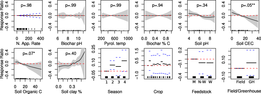
Figure 2. Estimated nonparametric smooth functions and parametric slope coefficients for factor variables, from model (1). Printed p-values are based on F-tests that  [48]. Shaded bands or dashed blue lines indicate 95% confidence intervals for the mean effect of each term. R2 averages 0.81 across 200 imputations. Figure S13 (available at stacks.iop.org/ERL/8/044049/mmedia) gives distributions of residuals (from each of the 200 fitted imputation models) for each datapoint, by study. The model is significantly different from a null model (with only random effects and no covariates) at p = 0.003.
Download figure:
Standard image High-resolution imageYield response was invariant to biochar type as parameterized by biochar pH, carbon content, and pyrolysis temperature. The benefit of manure biochar was higher on average than that of wood or nonwood biochar, but the effect was highly variable and not statistically significant. When fitting model (1) without observations from manure chars, or with only wood chars or only nonwood chars (not shown), results were nearly identical to results from models with all chars included together, though statistical confidence decreases due to smaller sample sizes. Similarly, while there was heterogeneity in response among crop types7 and experiment type (field versus greenhouse conditions), these differences were noisy and not significant.
Since soil properties predict yield response, spatially explicit analysis of where biochar is likely to have a greater or lesser benefit is possible using global databases of soil properties. Figure 2 projects our fitted model onto the ISRIC-WISE database of global-derived soil properties [22] for a nonwood biochar having median values of all biochar variables, and applying a dataset-median amount of nitrogen. Supplementary figure S14 (available at stacks.iop.org/ERL/8/044049/mmedia) gives the same map, with associated standard errors of fitted values. Values presented in figure 3 have the interpretation as our model's estimates of average plant response to biochar solely as a function of soil and biochar properties. Other factors that may influence yield response to biochar—such as heterogeneity between crop species, or differing biochar efficacy across different climates—may introduce bias in our effect estimates in model (1) or in our predictions in figure 3 if they are correlated with variables present in our model. In addition, our map abstracts from within-gridcell heterogeneity, and only presents spatially averaged estimates.

Figure 3. Model predictions for a median nonwood biochar applied to maize, projected onto spatially averaged soil property dataset from Batjes [22], in units of percentage relative increase. Areas with <5% of land in agriculture are masked using agricultural area extent data from Ramankutty [34]. Blue crosses give locations of studies used to fit the model.
Download figure:
Standard image High-resolution image
Given the global distribution of soil properties that we include in our model, our fitted model implies positive yield response over much of Sub-Saharan Africa, parts of South America, Southeast Asia, and southeastern North America. These areas are largely coincident with areas of highly weathered soils, generally in the tropics or subtropics. Our fitted model also implies that response in the belt to the north of Eastern Europe's chernozems would likely be positive. Yield response is predicted to be most negative in organic soils such as those in Indonesia, northern Eurasia and North America. Notably, our model implies that yield response may be weak and/or negative in many of the world's most important grain-producing areas, such as the Eurasian chernozems or central North American mollisols. Implications for South Asian vertisols, and in much of the North American corn belt near the great lakes, are predicted to be small to negative.
While our dataset gives good coverage over our parameter space (figures S1–S3 available at stacks.iop.org/ERL/8/044049/mmedia), geographic coverage is relatively poor in many regions. No studies have reported yield response to biochar in central North America, Eastern Europe/Eurasia, the Atlantic coast of South America, the African Sahel, or the South Asian peninsula. While soil properties characterizing these regions are represented in our dataset, our predictive maps should be viewed with caution where geographically out-of-sample predictions are being made.
4. Discussion
Our findings differ from previous meta-analyses of plant response to biochar, which used qualitative methods, univariate comparisons or complete-case regression analysis [3, 11–14]. Those studies found strong correlations between response ratio and soil pH, benefits in sandier soils, and stronger benefits in response to animal-derived biochars than plant-derived biochars. We find only suggestive evidence that soil pH influences response ratio, and suggestive evidence that soils with low reported clay content can expect weaker benefits to biochar application. While we estimate that response is higher in animal-derived biochars, the result is not significant. In contrast, our results emphasize the roles of soil cation exchange capacity and soil organic carbon content, with weaker emphasis on soil pH and opposite results for texture (as defined by reported soil clay content). Our estimates and ultimately our projection maps are consistent with biochar's benefits being maximized on weathered and degraded soils, which tend to have low cation exchange capacity, low soil organic carbon, low pH, and relatively non-reactive clay mineralogy. Somewhat surprisingly, we find little association between response ratio and biochar properties such as percentage carbon, pyrolysis temperature, or pH. Indeed, this lack of association (which is also apparent in bivariate scatterplots in figure S2 available at stacks.iop.org/ERL/8/044049/mmedia) suggests that if properties of biochars themselves are relevant in determining yield outcomes, the variables which we include in our model are of either unimportant, or potentially important only in mediating the influence of other variables. Explaining mechanisms by which different biochars influence yield outcomes remains an area for future research.
One of the more interesting and novel findings of our analysis is that biochar's yield benefits significantly increase over time, which was found individually in several studies in our dataset [16, 17, 35–38]. Many of these found slower rates of yield decline under continuous cultivation using biochar [16, 38], where both control and treatment yields declined after the initial season of implementation. This distinction between absolute increases versus slower decreases is important, and deserves further attention in future research. Response heterogeneity over time also warrants further research—our rather simple parametrization of time periods as uninteracted dummy variables captures only mean response over time8. However, plant response to biochar over time has important implications the economics of its use, and thereby its ability to contribute to climate change mitigation and improved agricultural productivity. Many biochar systems are costly in terms of labor or investment. Mechanisms underlying sustained/increased yield over time—along with improved quantitative understanding of biochar's retention [40–42] and decomposition within [6] soil—should improve understanding of the conditions under which biochar might be economically viable.
Finally, we present a few caveats to the interpretation of our results. First, we emphasize that our model presents average effects of our specified dependent variables on response ratio. While we find only small evidence for heterogeneous effects by crop or by biochar type, we are unable to exclude their presence. Second, our statistical approach will inevitably create misspecification bias: the predictor variables in our dataset are highly interactive in soil, yet we use them to fit an additively separable statistical model9. However, even when investigating a somewhat richer model with several interaction terms (equation S10, figures S16–S20 available at stacks.iop.org/ERL/8/044049/mmedia), results are largely consistent with this more simple model. We therefore favor the more parsimonious model for ease of interpretation. Furthermore, given that results from model S10 (available at stacks.iop.org/ERL/8/044049/mmedia) are generally somewhat larger, we favor the more parsimonious version as a more conservative lower bound on potential outcomes. Finally, predictions made from an imperfect model will inevitably propagate error. However, as the number of biochar experiments increases with time, statistical models specified based on a more detailed representation of biochar's dynamics in soil would represent a useful avenue for future research.
5. Conclusion
Our estimates suggest that biochar has a substantial and specific agroecological niche—on poor soils characterized by low cation exchange capacity, little soil organic carbon, and perhaps with lower pH and heavier textures. These characteristics describe many of the world's lowest-potential agricultural areas, which are predominantly found in the humid tropics. Given that many of the world's poorest agricultural soils exist in locations that are coincident with high rural poverty [45], our analysis invites further research on biochar's potential to play a role in agricultural development. Given that carbon mineralization from dead plant matter is generally faster in warm and moist conditions, biochar may represent a more effective means of carbon sequestration in the soils where it has the most agricultural benefit, than in soils where it has less benefit. This alignment however would depend on the degree to which biochar mineralization is dependent on environmental characteristics versus on its intrinsic chemistry, which for biochar remains poorly understood [6, 46].
Although areas for future research remain, given economically viable production technologies, technology adoption by potential beneficiaries, and an enabling policy environment, biochar systems appear to have potential to make a serious contribution to world food production, particularly in agricultural areas that are currently somewhat marginal in terms of global food production. Given increasing global food demand, this represents an important opportunity. While the economic viability of large-scale biochar systems remains to be demonstrated [47], substantial agronomic benefit over multiple years at relatively low application rates in certain regions indicates the possibility that some level of climate change mitigation via biochar systems could be achieved at negative cost.
Acknowledgments
This work was partly supported by the Director, Office of Science, Office of Biological and Environmental Research, Climate and Environmental Science Division, of the US Department of Energy under Contract No. DE-AC02-05CH11231 as part of the Terrestrial Ecosystem Science Program, as well as the Marie Curie CIG grant (No. GA 526/09/1762), and the Swiss National Foundation for Science. This work used the Extreme Science and Engineering Discovery Environment (XSEDE), which is supported by US National Science Foundation grant number OCI-1053575. We also acknowledge helpful comments from Professor Dr Michael W I Schmidt.
Footnotes
- 5
We note that our definition of 'clay content' is simply the clay content presented by authors of primary studies. Many primary studies do not differentiate between clay minerals and clay-sized particles, such as aluminum and iron oxides. Figure S18 (available at stacks.iop.org/ERL/8/044049/mmedia) presents an estimate of the effect of clay content (as defined by authors of primary studies) as mediated by soil CEC. We find suggestive evidence that high clay content is a driver of positive response to biochar particularly when cation exchange capacity is low.
- 6
This result reflects the respecification of N application rate as a linear term, because its estimation as a smooth function led to highly implausible estimates of extreme nonlinearity. Nonparametric estimates suggested sharply negative response ratios at low N applications and sharply positive ones near 100 kg N ha−1, before leveling to a modestly increasing function beyond 150 kg N ha−1. We therefore re-parameterized it as a linear parametric term. As such, it loses statistical significance.
- 7
Robustness checks are provided in SI (figure S15 available at stacks.iop.org/ERL/8/044049/mmedia) exploring heterogeneity in response to our predictor variables by crop type. Only very modest heterogeneity was found, supporting our specification of differences in response by crop as fixed indicator variables uninteracted with soil or biochar parameters.
- 8
In our dataset, the largest increases over control (>150%) beyond year 1 are from poor soils in Brazil [16] and Zambia [17]. Multi-year responses in other soils were generally in the 10–40% range. In one study that grew a mix of vegetables on a high-CEC, alkaline soil [39], plant response to biochar actually declined over time.
- 9
To name a few interactions, cation exchange capacity is determined both by clay mineralogy, soil organic matter, and pH. Biochar's surface charge is pH-dependent [43], and it is known to become encapsulated by clay particles in aggregates [44]. While its own pH tends to be high, the degree to which soil pH is affected by biochar will depend on buffering capacity.