
Abstract
The weekly dependence of pollutant aerosols in the urban environment of Lisbon (Portugal) is inferred from the records of atmospheric electric field at Portela meteorological station (38°47'N, 9°08'W). Measurements were made with a Bendorf electrograph. The data set exists from 1955 to 1990, but due to the contaminating effect of the radioactive fallout during 1960 and 1970s, only the period between 1980 and 1990 is considered here. Using a relative difference method a weekly dependence of the atmospheric electric field is found in these records, which shows an increasing trend between 1980 and 1990. This is consistent with a growth of population in the Lisbon metropolitan area and consequently urban activity, mainly traffic. Complementarily, using a Lomb–Scargle periodogram technique the presence of a daily and weekly cycle is also found. Moreover, to follow the evolution of theses cycles, in the period considered, a simple representation in a colour surface plot representation of the annual periodograms is presented. Further, a noise analysis of the periodograms is made, which validates the results found. Two datasets were considered: all days in the period, and fair-weather days only.
Export citation and abstract BibTeX RIS

Content from this work may be used under the terms of the Creative Commons Attribution 3.0 licence. Any further distribution of this work must maintain attribution to the author(s) and the title of the work, journal citation and DOI.
1. Introduction
The fair weather atmospheric electric field is dominated by the vertical component that is usually referred to as the vertical potential gradient (PG), defined in such a way that PG is positive in these conditions. In clean air, the global effect of thunderstorm activity can be apparent in the PG in the daily cycle known as the Carnegie curve (see for instance, Harrison 2013). Local effects arising from aerosol pollution contribute to additional variation in PG that may be very significant. Thus, in an urban environment it is expected that the PG at the ground, where the measurements are carried out, to be predominantly influenced by the combination of the effects of local pollution with those of the global atmospheric electric circuit. Pollution affects the PG through the following mechanism: pollutant aerosols remove small ions from the air that are very important to the atmospheric electric conductivity because they have high electric mobility; this removal causes the conductivity to decrease, therefore Ohm's law implies that the PG must increase (assuming that a fairly constant electric current is present between the ionosphere and the surface). In fact, for a constant aerosol size distribution it is shown that the PG is positively and linearly related with the aerosol particle mass concentration (Harrison and Aplin 2002). Such relation was further confirmed with measurements at Kew Observatory (Harrison 2006), where there is a long record of simultaneous measurements of PG and pollution levels. Baring this mind, it was discussed the possibility of using PG data to retrieve pollution levels (Manes 1977). Actually, such possibility is of great importance in sites that have historical PG data sets, but no pollution records are available, like the case of Western Scotland (Aplin 2012), where smoke emissions from industrial activity was inferred from Lord Kelvin's atmospheric electricity measurements. A similar situation occurs with the city of Lisbon, Portugal (figure 1), where PG measurements were made at Portela meteorological station from 1955, but reliable records of gas and particulate pollution started only in the 1990s. PG measurements were made from 1955 until 1990, but due to the radioactive fallout in the 1960s and 1970s (Pierce 1972) only the period of 1980–1990 can be correctly used in studies related with pollution. In fact, Lisbon is a polluted city and has a characteristic Mediterranean climate with fresh/rainy winter and a drought period during the summer (Andrade 1996). It is geographically located near the coast and presents topographical features, marked by a slightly rugged relief, associated with Serra de Monsanto with altitude of order 200 m on the west side, marked in figure 1, and the urban perimeter that shapes its climate (Alcoforado 1987). The surface wind regime is dominated by a northern strong flow (50% of observations), although it shows some annual variability, namely during the summer months while the winter records a greater dominance of NE, E, SW winds (Lopes 2003, Alcoforado et al 2006, 2008). At Portela (marked in figure 1) N, NW and NE winds prevail from May to September. The analysis of the summer winds frequency at the Portela airport for the period 1981–2000 shows that the winds blow from the NE, E, SE, S and SW, approximately 40% of the cases at midday; and at 18:00 h. Furthermore, N and NW winds, which together reach 52% at midday, increase their frequency up to 77% at 18:00 h. This is probably a consequence of the Tagus/Ocean breeze system due to temperature differences that develop between the continental atmosphere and estuarine or marine air (Alcoforado 1987) and Western sea breezes. Considering the air mass trajectory, the sea and estuary breezes transport, in most cases, cool and moist air with small ions (Serrano et al 2006a).

Figure 1. Left figure, geomorphology of Lisbon region with three main features marked: Serra de Monsanto, Baixa (city centre), and Portela Airport (location of the PG sensor). Right figure, the rectangle marks the geographical location of Lisbon in Portugal.
Download figure:
Standard image High-resolution imageMoreover, to consider the effect of pollution in urban measurements of PG, as it is the objective of the present paper, it is important to clarify the main cycles that affect pollutant aerosols. These cycles are imposed by the city dynamics and are expected be present in the PG records too. Three main possible cycles are listed below:
Daily cycle: two maxima are expected to appear, which correspond to the combined influences of urban pollution daily cycle and planetary influences (Harrison and Aplin 2002, Harrison 2009). One maximum shall develop in the early morning with the steep increase in city daily activities, followed by a decrease with the development of the boundary layer (intensification of the convective structures, ascending currents), while another shall occur in the evening, when the planetary influences intensify and then boundary layer convection weakens. Because the local PG is affected by the global variation of the electric field, it is necessary to remove this variation in order to properly observe the effect of the urban daily cycle.
Weekly cycle: at weekends (Saturdays and Sundays) urban activities decrease causing less pollution than in workdays (Mondays to Fridays). This notation will be used throughout the paper. Thus on weekends the PG is expected to be lower as compared with workdays, especially on Sundays (because pollutant aerosols generated during the workdays are significantly reduced by dry and wet depositions). In this way, this cycle can be linked exclusively to urban activities and for that reason it can be most useful to retrieve pollution historical records in the location where the PG measurements are made (Manes 1977).
Annual cycle: the spring/summer months are expected to have lower concentration of pollution near the ground, because of the reduction in traffic levels (especially during the holiday time), but also the increase of altitude of the convective boundary layer. In fact, this cycle is dominated by seasonal variations (Reddell et al 2004) related with the development and weakening of the convective boundary layers in spring/summer and fall/winter, respectively. Such variations mask the effect of urban activity changes and one way of overcoming this is to look for seasonal variation in the weekly cycle.
In fact, the influence of pollution weekly dependence in urban environmental processes is now receiving a significant research effort (Williams and Mareev 2014). The verification of the weekend effect in lightning (Bell et al 2009), rainfall (Bell et al 2008), both hail and tornadoes (Rosenfeld and Bell 2011), and diurnal temperature (Forster and Solomon 2003) reveals the importance of studying this cycle and the necessity of further research.
With that purpose this paper investigates the signature caused by the weekly cycle in pollution on the PG recorded at Portela. Other effects have been previously studied in this set of data: cosmic radiation, artificial radioactivity, and aerosol concentration (Serrano et al 2006a); relative humidity and wind intensity (Serrano et al 2006b); seismic activity (Silva et al 2012); but, this is the first study addressing pollution.
2. Data
Mean hourly PG values were registered at the Portela meteorological station (Lisbon, Portugal; 38°47'N, 9°08'W) in the period from 1955 to 1990. These measurements were made using a Bendorf electrograph coupled to a radioactive probe (securing equality of potential between the sensor and the air; improving the time response) installed at 1 m height from a cement base on the ground. The measurements were interrupted from 1975 to 1977 when the electrometer was stopped for maintenance. Its sensitivity was checked using an electronic electrometer with standard voltage source between ± 200 V and the same calibration procedure was used in all periods of operation. A report made by the National Service of Meteorology compiles this information (Figueira 1965). In the present study only the period from 1980 to 1990 is considered and two situations are studied: all weather PG (AW), which includes the entire PG dataset; and fair-weather PG (FW), selected as those hours with cloudiness less than 0.3, wind speed less than 20 km h−1 and absence either of both fog or precipitation. More details of the dataset can be found in the study of Serrano et al 2006a.
Figure 2(a) shows the monthly mean values and the corresponding standard deviations of the PG in AW and FW conditions for the period considered. Figures 3(a) and (b) show boxplots for these data (marked as 'whole week') without outliers. Moreover, a summary of statistical parameters is presented in table 1. It is clearly seen that the PG for AW (mean, 84.73 V m−1) tends to be lower than for FW (mean, 94.27 V m−1), most probably because of the influence of the negative outliers as is clear from the significant kurtosis value for AW, 13.365, as compared with the FW, 7.710. This is also consistent with the skewness parameters found, as AW values are less positively skewed, 1.031, than FW, 1.725. The annual behaviour of the PG for AW and FW conditions (shown in figure 4(a)) demonstrate that summer months have the lowest mean values and standard deviations (August for AW and June for FW); January has the highest for both AW and FW. Moreover, there is no visible trend in the mean PG values per year for AW and FW (empty circles), shown in figure 5(a). It is important to mention that FW dataset has two drawbacks: it has significantly less data than the AW dataset (number of days given in table 1), and it is difficult to find FW values of PG for a complete week and for this reason comparison is made between values for workdays and weekends that do not necessarily correspond to the same week. This implies that the results for FW data are not so statistically reliable compared with AW in respect to the study of the weekly cycle.
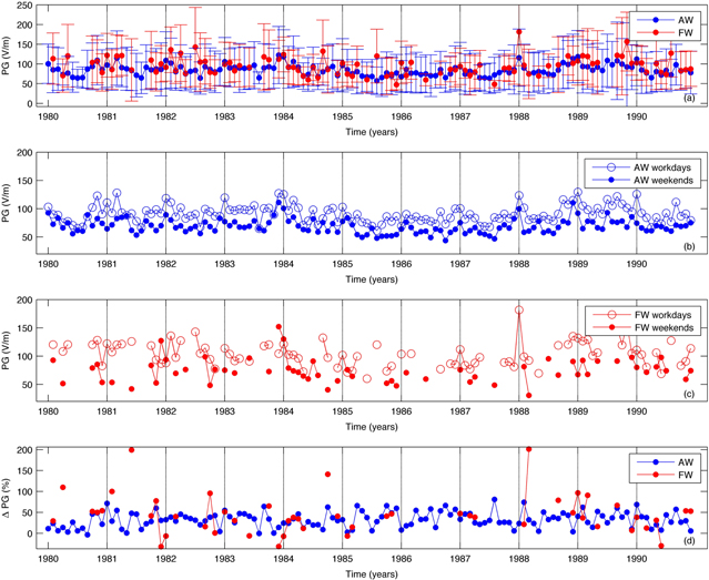
Figure 2. Mean monthly values of PG measured from Portela during the period from 1980 until 1990: (a) PG for AW and FW (error bars represent standard deviations); (b) AW workdays and weekends PG; (c) FW workdays and weekends PG; (d) AW and FW-PG relative difference between workdays and weekends, ΔPG.
Download figure:
Standard image High-resolution image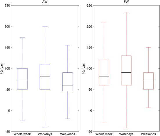
Figure 3. Boxplot of hourly PG values for AW (blue): whole week, workdays, and weekend; boxplot for FW (red): whole week, workdays, and weekends. A black line in all boxes marks median and the outliers are not presented.
Download figure:
Standard image High-resolution imageTable 1. Mean, median, standard deviation, skewness, kurtosis, and number of days for the period between 1980 and 1990. The atmospheric electric field measurements are divided in: AW whole week, AW workdays, AW weekends, FW whole week, FW workdays, and FW weekends.
| AW whole week | AW workdays | AW weekends | FW whole week | FW workdays | FW weekends | |
|---|---|---|---|---|---|---|
| Mean (V m−1) | 84.73 | 90.87 | 69.39 | 94.27 | 101.72 | 73.49 |
| Median (V m−1) | 72.32 | 80.00 | 60.00 | 80.00 | 90.00 | 70.00 |
| Standard deviation (V m−1) | 54.81 | 58.64 | 39.88 | 54.96 | 59.35 | 32.11 |
| Skewness | 1.031 | 1.039 | −0.1790 | 1.725 | 1.549 | 1.023 |
| Kurtosis | 13.364 | 11.180 | 29.25 | 7.710 | 6.671 | 4.972 |
| Number of days | 4018 | 2870 | 1148 | 356 | 262 | 94 |
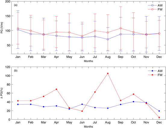
Figure 4. Annual behaviour of: (a) PG for AW and FW; (b) ΔPG for AW and FW. Error bars represent standard deviations.
Download figure:
Standard image High-resolution image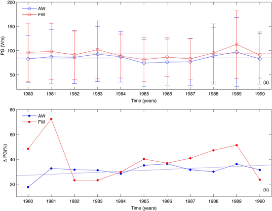
Figure 5. Annual averages from 1980 until 1990: (a) PG for AW and FW; ΔPG for AW and FW. Error bars represent standard deviations.
Download figure:
Standard image High-resolution image3. Methodology
Relative difference method: an initial comparison is made between the normalized distributions of the PG for workdays and weekends for both AW and FW datasets. Furthermore, to quantify the effect of the weekly cycle the relative difference between the mean PG for workdays (Mondays to Fridays), PGworkdays, and for weekends (Saturdays and Sundays), PGweekends, is calculated using the equation: ΔPG (%) = (PGworkdays/PGweekends − 1) × 100%. This formula is similar to the one used by Sheftel et al 1994 that considers the ratio of the PG for workdays and for Sundays. Such a formulation was used previously to study the weekly effect on the electric conductivity of air (Tammet 2009). Three average procedures for PGworkdays and PGweekends are made: average per month (monthly means); average values that correspond to the same month for all years, e.g. the values of all Januaries in 1980–1990 (annual behaviour); average per year (annual means).
Lomb–Scargle periodogram (LSP) technique: was developed for interrupted data sets in astrophysics (Lomb 1976, Scargle 1982), and has been extensively used in atmospheric science (Schulz and Stattegger 1997, Hocke and Kampfer 2009). The LSP is similar to the Fourier transform, but it estimates the frequency spectrum based on a least squares fit of the sinusoids. In fact, the LSP spectrum converges to Fourier transform spectrum in the limit of evenly spaced observations. The LSP provides the significant frequencies and their respective amplitudes (in a statistical sense) enabling a proper evaluation of the dominant periods that influence the data. In this context, fair-weather PG is an unevenly distributed time series and for that reason its spectral analysis must be made using the LSP technique, e.g. (Xu et al 2013). The programme used in the present study is an LSP implementation (Press et al 1992), which was developed in MATLAB® (Brett 2001). The periodogram for the entire data sets has been calculated. Moreover, to follow the evolution of the dominant periods (less than a year) the LSP is calculated for each year (with a 2 h resolution that is twice the sampling time, according to Nyquist theorem), and the periodograms plotted in a colour surface plot. To do this, estimation of the spectral amplitudes with respect to the same periods for all the years was considered. Thus a vector was created with logarithmically spaced values from the initial period (always above the inverse of the Nyquist frequency) until the final period (always below one year) and interpolated the values of the smoothed periodograms (moving averages of five values) using cubic spline interpolation. In this way, dominant periods appeared as horizontal lines across the plot. The results were further confirmed by a noise analysis.
4. Results and discussion
Figures 2(b) and (c) demonstrate that PG values at the weekends tend to be lower than the values for workdays, both for AW and FW. Actually, the monthly values of ΔPG, figure 2(d), are generally positive. This observation is confirmed by the distributions of PG values for workdays and weekends. The boxplots, figures 3(a) and (b), show that the weekends have inter quartile ranges smaller than the ones for workdays, for both AW and FW. Descriptive statistical parameters are presented in table 1. These show the following:
- (1)AW, mean values of PG for workdays, 90.87 V m−1, is higher than for weekends, 69.39 V m−1, the relative difference is 31.00%. PG for workdays has a broader distribution, is more positively skewed and less prone to outliers than weekends.
- (2)FW, PG shows a similar tendency, mean values for workdays, 101.72 V m−1, higher than for weekends, 73.49 V m−1, the relative difference is 38.41%. Workdays PG has a boarder distribution, is more positively skewed and more prone to outliers than weekends.
The high relative differences statistically prove the existence of a week dependence of the PG, both for AW and FW. Actually, Israelsson and Tammet (2001) at Marsta Observatory, located in a rural region (10 km North of Uppsala, Sweden), measured air conductivities and calculated the relative differences using Sheftel formulation (Sheftel et al 1994). The relative differences they found are much lower than the relative differences found here for PG. Such disparity reveals the importance that urban pollution has on PG measurements.
Additionally, figure 4(b) reveals that ΔPG has an annual behaviour different from PG (AW and FW). Interestingly, ΔPG shows a minimum in December which is the month of the year with less urban activity (specially traffic) because of Christmas holidays. During the rest of the year, ΔPG behaviour for AW appears to be more consistent with urban activity. Actually, it decreases from January until August (summer holidays) and increases again until October (a month with significant urban activity) decreasing again until December. On the contrary, ΔPG for FW has an increasing tendency from January until August and after that decreases. The reason for this is probably lack of FW data, as discussed above.
Finally, the trend for annual averages of ΔPG (AW and FW) is shown in figure 5(b). Again, the behaviour of AW and FW values of PG differ; AW shows an increasing trend and no trend is evident for FW. The tendency of ΔPG for AW is in accordance with the population growth in the metropolitan area of Lisbon in the considered period. According to the Portuguese National Statistics Institute (INE 2011), the population in the metropolitan area of Lisbon has grown until the 1980s and stabilized in the 1990s. Actually, the most significant population growth occurred in the 1970s and the reason for that was the Portuguese democratic revolution of 25 April 1974. Thus after it and until 1976 an important growth in the Portuguese population occurred due to the return of many immigrants from the former Portuguese colonies of Africa, as those nations claimed their independence (Moreira and Rodrigues 2008). As a consequence of such increase in population there was an increase in urban pollution; which was mainly due to traffic intensification and industrial activity. In fact, the social processes involved in this relation of population growth and pollution level was intensively studied, e.g. (Constant et al 2014) and links the demographic growth of the 1980s in Lisbon region with the development of the weekly cycle in the PG values. This relation adds a socioeconomic dimension to the studies of PG in urban regions as discuss in other works (Aplin 2012).
Figures 6(a) and (b) show LSPs calculated from PG data for AW and FW, respectively. As expected the periodogram for AW contains more harmonic components than the FW one, especially for lower periods. The occurrence of two main cycles, daily, and weekly cycles, is evident in both data sets. Additionally, PG for AW shows two other cycles: an annual cycle caused by the seasonal meteorological variations, and half-day cycle (12 h period) likely to be related to traffic pollutant aerosols. Tchepel and Borrego (2010) have shown the presence of a significant influence of short-term fluctuations (12 h and 24 h periods) to the variance of both CO and PM10 measured in urban environments. Those authors confirmed the contribution of traffic as the pollutant source using cross-spectrum analysis; which showed a correlation percentage from 45% to 70% between the pollutant concentrations and traffic dynamics (Tchepel and Borrego 2010). Besides the main peaks mentioned, LSP in the AW case presents a myriad of other smaller peaks between the main ones; which are their sub-harmonics (Xu et al 2013).

Figure 6. Lomb–Scargle periodograms calculated using the LSP implementation in MATLAB (Brett 2001) for 1980–1990: (a) AW; (b) FW. The following parameters were used hifac = 1 (that defines the frequency limit as hifac times the average Nyquist frequency), ofac = 4 (oversampling factor), and no calibratation is done to the data.
Download figure:
Standard image High-resolution imageTo further clarify the evolution of the weekly cycle during the period of study, figures 7(a) and (b) show colour surface plots of the LSP using the procedure described previously. It is important to mention that due to the variation in the number of FW days, the band of periods observable in each year varies considerably; in the worst case, the periods accessible were above 1.63 days. For that reason the colour surface plot for FW, figure 7(b), is restricted to periods above 3.162 days. In the AW case periods start at ∼0.316 days (an order of magnitude lower). The amplitude is represented in a colour map as a function of the period (y axis) for the 11 years of analysed data (x axis). For AW, figure 7(a), the daily and weekly cycles are clearly seen by two horizontal red lines (labelled with the respective cycle) and confirm the persistence of the weekly cycle during the 1980s and beginning of the 1990s. In contrast, the colour surface plot for FW, figure 7(b), does not show the weekly cycle so clearly. Nevertheless, it is seen that the spectrum for 1986 responds most appreciably to low periods as compared to the other years (red blurs below the weekly cycle). This behaviour can be tentatively related with the impact of Chernobyl nuclear accident (26 April 1986) on the global electric circuit (Takeda et al 2011); study of this effect is out of the scope of the present work.
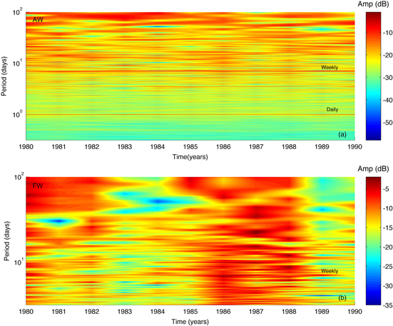
Figure 7. Colour surface plot of Lomb–Scargle periodograms for each year: (a) AW; (b) FW.
Download figure:
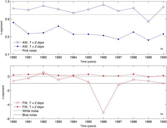
Standard image High-resolution imageThe consistency of the colour surface plots is confirmed by noise analysis of the LSP (Tuzlukov 2002). This calculates, for each LSP, the n-exponent defined as a power law dependence of the power spectral density, S(T), with the period, T, of the type, S(T) ∝ Tn. The spectra are split into two parts: periods shorter than two days (twice the dominant 1 day period), and periods longer than two days. The exponents for periods shorter than Tc = 2 days are shown to be higher than exponents that correspondent to longer periods. For AW, figure 8(a), the n-exponents for T < Tc are close to the 1/f noise (pink noise); this type of noise is present in many systems in nature and is of special interest (Dutta and Horn 1981). Complementary, the n-exponent for T > Tc diminishes over the studied years down to 0.5. It is argued that such decreasing tendency (the opposite trend of ΔPG for AW) must be related with the increase in Lisbon pollution levels. Seen in this way, pollution causes a spread of spectral power for periods longer than Tc and tends to flatten the spectra. In fact, it is known that long-range transport of the pollution contributes to pollutant aerosols spectra at high periods (Tchepel and Borrego 2010). Additionally, because of the mentioned variation in the number of FW days per year it is difficult to properly study the evolution of the n-exponent for periods shorter than Tc = 2 days in this case. For these periods n tends to be negative, around −1 (blue noise), and has an anomalously low value for 1986. The negative values of n reveals that the PG responds better to processes with lower-periods and contradicts the behaviour found for AW; this could be related with local perturbations that have typically small periods, e.g. the half-day cycle (Xu et al 2013). Nevertheless, the analysis of n for periods above Tc is found to have values near from, but not zero (white noise, n = 0). This is consistent with the behaviour found in the AW case for periods above Tc. Again this fact can be interpreted by a spread of power in the complete spectral band.
Figure 8. Noise upper panel: evolution of the n-exponent from the Lomb–Scargle periodograms shown in figures 6 and 7, along the years for period below Tc = 2 days (empty circle) and above 2 days (full circle): (a) AW; (b) FW.
Download figure:
Standard image High-resolution image
5. Conclusions
This work clearly demonstrates the existence of a weekly dependence on the PG recorded at Portela (Lisbon, Portugal) that is related with the weekly cycle of urban pollution, mainly due to traffic. This dependence was confirmed through a statistical analysis that shows a relative difference of PG values for working days and weekends of 31.00% and 38.41% for AW and FW, respectively. The annual average of the relative difference shows an increasing trend in the period studied. Additionally, the spectra show a significant peak for the weekly period that confirms the existence of the weekly cycle, as well as a 12 h periodicity present in the PG data, attributed to traffic pollution. Spectral noise shows that spectra tend to flatten along the studied period. These aspects are consistent with the evolution of the weekly cycle of pollution due to the rise in pollutant aerosol concentrations caused by the increase of traffic in Lisbon.
As a final remark, it is important to mention that this 7-day periodicity is in the range of periods of the known seismic precursors (Silva et al 2012) and for that reason the effect of urban pollution should be carefully taken into account in those studies.
Acknowledgments
Hugo Silva acknowledges the support of two Portuguese institutions: the Fundação para a Ciência e a Tecnologia (FCT) for the Post-Doctoral fellowship, SFRH/BPD/63880/2009, and the Fundação Calouste Gulbenkian for the award Estímulo à Criatividade e à Qualidade na Actividade de Investigação in the science program of 2010. Marta Melgão also thanks the support of FCT through the PhD fellowship, SFRH/BD/89218/2012. Researchers from the Geophysics Centre of Évora acknowledge the funding provided by the contract with FCT, Pest/OE/CTE/UI0078/2014. The authors are grateful to Claudia Serrano, Mourad Bezzeghoud, Maria João Costa, Luísa Nogueira, and Manuela Oliveira for their support in many aspects that contributed to this study, and are in indebted to Samuel Bárias for his technical support on the data usage. Especially acknowledgments are given to Doctor Mário Figueira for recording the PG for more than 30 years; without him this study would not be possible.