

Abstract
Crop yields are critically dependent on weather. A growing empirical literature models this relationship in order to project climate change impacts on the sector. We describe an approach to yield modeling that uses a semiparametric variant of a deep neural network, which can simultaneously account for complex nonlinear relationships in high-dimensional datasets, as well as known parametric structure and unobserved cross-sectional heterogeneity. Using data on corn yield from the US Midwest, we show that this approach outperforms both classical statistical methods and fully-nonparametric neural networks in predicting yields of years withheld during model training. Using scenarios from a suite of climate models, we show large negative impacts of climate change on corn yield, but less severe than impacts projected using classical statistical methods. In particular, our approach is less pessimistic in the warmest regions and the warmest scenarios.
Export citation and abstract BibTeX RIS

Original content from this work may be used under the terms of the Creative Commons Attribution 3.0 licence. Any further distribution of this work must maintain attribution to the author(s) and the title of the work, journal citation and DOI.
1. Introduction
Anthropogenic climate change will affect the agricultural sector more directly than many others because of its direct dependence on weather (Porter et al 2013). The nature and magnitude of these impacts depends both on the evolution of the climate system, as well as the relationship between crop yields and weather. This paper focuses on the latter—yield prediction from weather. Accurate models mapping weather to crop yields are important not only for projecting impacts to agriculture, but also for projecting the impact of climate change on linked economic and environmental outcomes, and in turn for mitigation and adaptation policy.
A substantial portion of the work of modeling yield for the purpose of climate change impact assessment relies on deterministic, biophysical crop models (e.g. Rosenzweig et al 2013). These models are based on detailed representations of plant physiology and remain important, particularly for assessing response mechanisms and adaptation options (Ciscar et al 2018). However, they are generally outperformed by statistical models in prediction over larger spatial scales (Lobell and Burke 2010, Lobell and Asseng 2017). In particular, a large literature following Schlenker and Roberts (2009) has used statistical models to demonstrate a strong linkage between extreme heat and poor crop performance. These approaches have relied on classical econometric methods. Recent work has sought to fuse crop models with statistical models, variously by including crop model output within statistical models (Roberts et al 2017), and by using insights from crop models in the parameterization of statistical models (Roberts et al 2012, Urban et al 2015).
In parallel, machine learning (ML) techniques have advanced considerably over the past several decades. ML is philosophically distinct from much of classical statistics, largely because its goals are different—it is largely focused on prediction of outcomes, as opposed to inference into the nature of the mechanistic processes generating those outcomes. (We focus on supervised ML—used for prediction—rather than unsupervised ML, which is used to discover structure in unlabeled data.)
We develop a novel approach for augmenting parametric statistical models with deep neural networks, which we term semiparametric neural networks (SNN). Used as a crop yield modeling framework, the SNN achieves better out-of-sample predictive performance than anything else yet published. By using prior knowledge about important phenomena and the functional forms relating them to the outcome, the SNN substantially improves statistical efficiency over typical neural networks. By augmenting a parametric model with a neural network, it captures dynamics that are either absent or imperfectly specified in parametric models. Specifically, we nest linear-in-parameters regression specifications—taken from the yield and climate modeling literature—within the top layer of the network (figure 1). Together with a variety of complementary methods discussed below, this improves efficiency and ultimately performance over both extant parametric approaches, and over fully-nonparametric neural networks.

Figure 1. Schematic drawing of a (semiparametric) neural network. Neural networks use a form of representation learning (Bengio et al 2013). Left: low-level sensory data Z is aggregated into progressively more abstract derived variables V through parameters (lines) and nonlinear transformations (see equation (2)). '1' represents the 'bias' term—akin to an intercept in a linear regression. Right: a stylized agricultural example of aggregation of sensory data into progressively more abstract representations. Bottom: a semiparametric neural net with cross-sectional fixed effects α and linear terms X. Acronyms/abbreviations: temp = temperature, precip = precipitation, VPD = vapor pressure deficit, GDD = growing degree days.
Download figure:
Standard image High-resolution imageBeyond our application to crop yields, this approach provides a general framework for improving the predictive skill of any neural network for which there is extant prior knowledge about the nature of the data-generating process, which can be captured by a model specification that is informed by domain-area theory and/or expertize.
We find that the choice of yield model affects the severity of climate change impact projections, with differences in the yield decline from baseline between SNN and OLS projections greater than 16 percentage points in some of the most severe projections. Also, while OLS projections suggest yield increases in some northerly areas in some of the less severe scenarios, this projection is largely absent in the SNN projections. Finally, confidence intervals for mean projections are much smaller for the SNN than for the equivalent OLS regression, implying greater precision for any given weather scenario (figure B2).
The remainder of this paper describes the model (section 2), data (section 3), results (section 4), and concludes with a discussion (section 5). Methods are detailed in (section 6).
2. Model
2.1. Parametric yield model
Absent stresses, plant growth is strongly related to the accumulation of time exposed to specific levels of heat. This can be measured by the growing-degree day (GDD), which measures the total amount of time spent within a particular temperature range. The main models used by Schlenker and Roberts (2009) were OLS regressions in GDD, along with fixed effects and controls, similar to the following:

where r is the range of each GDD bin, and X includes a quadratic in precipitation as well as quadratic time trends, included to account for technological change.
This model allows different temperature bands to have different effects on plant growth, and exposed large negative responses to temperatures about 30°C in maize when first reported. Subsequent work has identified the role of vapor pressure deficit (VPD) in explaining much of the negative response to high temperatures (Roberts et al 2012), developed a better statistical representation of the interplay of water supply and demand (Urban et al 2015), and documented the decreasing resilience to high VPD over time (Lobell et al 2014).
Developed for the purpose of statistical inference about critical temperature thresholds, models such as (1) leave room for improvement when viewed as purely predictive tools. Its implicit assumptions—additive separability between regressors, time-invariance of the effect of heat exposure, and omission of other factors that may affect yields—improve parsimony, interpretability, and thereby understanding of underlying mechanisms. But they will bias predictions to the degree that they are incorrect in practice, as will any simple specification of a complex phenomenon. Rather than replacing these models entirely however, we adapt ML tools to augment them.
2.2. Neural nets and semiparametric neural nets
Artificial neural networks—first proposed in the 1950s Rosenblatt (1958)—employ a form of representation learning (Bengio et al 2013). Input data—here in the form of raw daily weather data with high dimension and little direct correlation with the outcome—are progressively formed into more abstract and ultimately useful data aggregates. These are then related to an outcome of interest (figure 1). Importantly, these aggregates are not pre-specified, but rather they are discovered by the algorithm in the process of training the network. It is the depth of the successive layers of aggregation and increasing abstraction that give rise to the term 'deep learning' (LeCun et al 2015).
A basic neural network can be defined by equation (2):
Terms Vl are derived variables (or 'nodes') at the lth layer. The parameters  map the data Z to the outcome. The number of layers and the number of nodes per layer is a hyperparameter chosen by the modeler. Matrices
  are of dimension equal to the number of nodes of the lth layer and the next layer above.
The 'activation' function  is responsible for the network's nonlinearity, and maps the real line to some subset of it. We use the 'leaky rectified linear unit' (lReLU) (Maas et al 2013):
which is a variant of the ReLU:  . ReLU's were found to substantially improve performance over earlier alternatives when first used (Nair and Hinton 2010), and the leaky ReLU was found to improve predictive performance in our application.
The top layer of equation (2) is a linear regression in derived variables. Recognizing this, the basic innovation employed here is simply to add linear terms as suggested by prior knowledge, and cross-sectional fixed effects to represent unobserved time-invariant heterogeneity. If such terms are X and α respectively, the model becomes
with i and t indexing individuals and time. This allows us to nest equation (1) within equation (2)—incorporating parametric structure where known (or partially-known), but allowing for substantial flexibility where functional forms for granular data are either not known or are known to be specified imperfectly.
Methods that we use for training semiparametric neural networks are detailed in the methods section, and implemented in the panelNNET R package2 .
3. Data
We focus on the states of Illinois, Indiana, Iowa, Kentucky, Michigan, Minnesota, Missouri, Ohio, and Wisconsin. These were chosen because they are geographically contiguous and capture a large proportion of non-irrigated corn production in the US. County-level corn yields from 1979 through 2016 were taken from the US National Agricultural Statistics Service (NASS) QuickStats database (NASS 2017). In addition, we extract data from QuickStats on the proportion of each county that is irrigated, formed as an average for each county of the reported area under irrigation in the past three USDA censuses of agriculture (2002, 2007, 2012).
Historical weather data is taken from the gridded surface meteorological dataset (METDATA) of Abatzoglou (2013). Variables are observed daily and include minimum and maximum air temperature and relative humidity, precipitation, incoming shortwave radiation (sunlight), and average wind speed. An overview of the variables used is presented in table 1. We note that all variables that are included parametrically are also included nonparametrically, with the exception of the quadratic terms in time and total precipitation. This allows for a parametric 'main effect,' while also allowing these variables to form nonlinear combinations with other input data, which could be useful if the effects of these variables depend partially on the levels of other variables. When training the model, we convert all nonparametric covariates into a matrix of their principal components, retaining those that comprise 95% of the variance of the data.
Table 1. Variables used in yield model.
| Phenomenon | # Terms | Type | Description |
|---|---|---|---|
| Precipitation | 245 | Nonparametric | Daily precipitation |
| Air temperature | 490 | Nonparametric | Daily minimum and maximum air temperature |
| Relative humidity | 490 | Nonparametric | Daily minimum and maximum relative humidity |
| Wind speed | 245 | Nonparametric | Daily average wind speed, taken as the Euclidean norm of northward and eastward wind as reported by METDADA and MACA |
| Shortwave radiation | 245 | Nonparametric | Daily total solar radiation |
| Growing degree-days | 42 | Both | Cumulative time at 1°C temperature bands, from 0–40. Additional bins capture the proportion of time spent below 0°C and above 40°C. These terms enter both the parametric (linear) and nonparametric (neural network) portions of the yield model |
| Total precipitation | 2 | Parametric | Total precipitation over the growing season, and its square |
| Latitude/longitude | 2 | Nonparametric | County centroids |
| Time | 1 (2) | Both | Year enters as a quadratic time trend in the parametric (linear) portion of the model, and as a nonparametric term at the base of the neural network |
| Soil | 39 | Nonparametric | Percentages sand/silt/clay, organic matter, particle density, K saturation, available water capacity, erodibility factors, electrical conductivity, cation exchange capacity, pH (in H2O and CaCl2), exchangeable H+, slope (gradient and length), loss tolerance factor, elevation, aspect, albedo (dry), minimum bedrock depth, water table depth minimum (annual and Apr–Jun), ponding frequency, available water storage, irrigated and non-irrigated capability class (dominant class and percentage), root zone available water storage and depth |
| Proportion irrigated | 1 | Nonparametric | Proportion of the county's farm land under irrigated production |
| County | 1 (201) | Parametric | Indicator variable for each of 201 counties in Iowa and Illinois (estimated as a fixed effect via the 'within transformation' at the top later of the network) |
Future weather simulation data is taken from the Multivariate Adaptive Climate Analogs (MACA) dataset (Abatzoglou and Brown 2012), which is a statically downscaled set of projections from a suite of climate models comprising the coupled model intercomparison project (CMIP5) (Taylor et al 2012). Individual models used in this analysis include MRI-CGCM3 (Yukimoto et al 2012), GFDL-ESM2M (Dunne et al 2012), INMCM4 (Volodin et al 2010), CNRM-CM5 (Voldoire et al 2013), BNU-ESM (Ji et al 2014), IPSL-CM5A-LR and IPSL-CM5A-MR (Dufresne et al 2013), BCC-CSM1-1-m (Xin et al 2012), CanESM2 (Chylek et al 2011), MIROC-ESM-CHEM (Watanabe et al 2011), HadGEM2-ES365 and HadGEM2-CC365 (Collins et al 2011). All models from the MACA dataset were selected for inclusion where they reported all variables used in table 1. Where a single group produced more than one model, older versions were dropped unless they were substantially qualitatively different in their representaiton of the Earth system.
Each model simulates RCP4.5 and RCP8.5—two emissions scenarios representing modest climate change mitigation and business-as-usual emissions, respectively. Both METDATA and MACA are provided at 4 km2 resolution. We aggregate these data as county-level averages, weighted by the proportion of each 4 km gridcell that is farmed, taken from NASS's Cropland Data Layer (Johnson et al 2009). We exclude observations outside of the growing season, using weather from March through October. In addition to weather data, we use county-level soil data, taken from the Soil Survey Geographic (SSURGO) Database (Soil Survey Staff 2017). This dataset comprises 39 measures of soil physical and chemical properties.
A complete description of the modeling approach is in the methods section, below. We make use of bootstrap aggregation, or 'bagging' (Breiman 1996) to both reduce the variance of predictions and to estimate out-of sample prediction error. Models (1) and (3) are fit to 96 bootstrap samples of unique years in our dataset, and error is assessed as the average of the years not in the bootstrap sample.
4. Results
4.1. Predictive skill
We begin by comparing the accuracy of the various approaches in predicting yields in years that were not used to train the model; table 2. The accuracy of the parametric model and the SNN was substantially improved by bagging, but the bagged SNN performed best. The fully-nonparametric neural net—which was trained identically to the SNN but lacked parametric terms—performed substantially worse then either the OLS regression or the SNN.
Table 2. Out-of-sample error estimates. For bagged predictors, a year's prediction was formed as the average of predictions from each bootstrap sample not containing that year, and the averaged out-of-sample prediction was compared against the known value. For unbagged predictors, the mean-squared error of each of the out-of-sample predictions was averaged.
| Model | Bagged |

|
|---|---|---|
| Parametric | No | 367.9 |
| Semiparametric neural net | No | 292.8 |
| Parametric | Yes | 334.4 |
| Fully-nonparametric neural net | Yes | 638.6 |
| Semiparametric neural net | Yes | 251.5 |
That bagging improves model fit—of both the OLS regression and the SNN—implies that certain years may have served as statistical leverage points, and as such that un-bagged yield models may overfit the data. This is because there are too few distinct years of data to determine whether the heat of an anomalously hot year is in fact the cause of that year's anomalously low yields. If bootstrap samples that omit such years estimate different relationships, then averaging such estimates will reduce the influence of such outliers.
That the SNN and the OLS regression both substantially out-perform the fully-nonparametric neural net is simply reflective of the general fact that parametric models are more efficient than nonparametric models, to the degree that they are correctly specified. That the SNN is more accurate than the OLS regression—but not wildly so—implies that model (1) is a useful but imperfect approximation of the true underlying data-generating process.
The spatial distribution of out-of-sample predictive skill—averaged over all years—is mapped in the online supplementary material at stacks.iop.org/ERL/13/114003/mmedia.
4.2. Variable importance
It can be desirable to determine which variables and groups of variables contribute most to predictive skill. Importance measures were developed in the context of random forests (Breiman 2001). Applied to bagged estimators, these statistics measure the decline in accuracy when a variable or set of variables in the out-of-bag sample is randomly permuted. Random permutation destroys their correlation with the outcome and with variables with which they interact, rendering them uninformative. We compute these measures for each set of variables as the average MSE difference across five random permutations.
These are plotted in figure 2. Of the daily weather variables, those measured in mid-summer are most important by this measure, particularly daily precipitation and minimum relative humidity during the warmest part of the year. The later is consistent with findings of Anderson et al (2015) and Lobell et al (2013), who show that one of the main mechanisms by which high temperatures affect yield is through their influence on water demand.
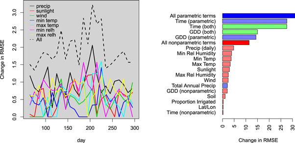
Figure 2. Variable importance measures, for time-varying variables (left) and time-invariant variables and whole sets of time-varying variables (right). Red (blue) [green] bars indicate variables that enter nonparametrically (parametrically) [both].
Download figure:
Standard image High-resolution imageThe parametric portion of the model is more important than the nonparametric part of the model (figure 2, right)—mostly through the incorporation of parametric time trends, but also through GDD. The nonparametric component of the model—taken as a whole—is less important than the parametric representation of GDD, though nonetheless responsible for the improvement in predictive skill over the baseline OLS regression. However, the predictive power of the time-varying temperature variables lends support to the findings of Ortiz-Bobea (2013), who notes that there is room for improvement in the additive separability approximation implicit in the baseline parametric specification. Soil variables, proportion of land irrigated, and geographic coordinates have low importance values. It is possible that these variables would be more important in a model trained over a larger, less homogeneous area—allowing them to moderate and localize the effects of daily weather variables. The centrality of time trends to predictive skill explains the poor performance of the fully-nonparametric neural net.
4.3. Projections
Projections for the periods 2040–2069 and 2070–2099, for both RCPs and all climate models, are reported in figure 3. Plotted confidence intervals are derived by averaging the pointwise standard errors of a smoothing spline applied to the underlying time series of projected yields, and as such reflect projected interannual variability. These projections make no assumptions about technological change, inasmuch as the value of the time trend is fixed at the year 2016 for the purpose of prediction. As such, projections only reflect change in response to weather, assuming 2016s technology and response to weather. Nor do we model adaptation or carbon fertilization. Omission of these factors is likely to bias statistical projections downwards, to the degree that these factors will increase expected yields, though we note that recent research raises uncertainty about the magnitude or existence of the CO2 fertilization effect (Obermeier et al 2018).

Figure 3. Yield projections, averaged over the study region, by climate model. Line segment length reflects 95% confidence intervals for mean projections, based on projected interannual yield variability. Confidence intervals reflecting uncertainty in estimated average projections of yield given weather presented in figure B.2. Dotted line reflects (detrended) historical average yields.
Download figure:
Standard image High-resolution imageWhile there is little difference between the models in scenarios in which yields decline less, the SNN projects substantially less-severe impacts in scenarios where yields decline the most across all models, including most of the models in 2070–99 under RCP8.5. Notably, the bagged OLS specification is nearly always less pessimistic than the standard OLS model. It is likely that the pessimism of OLS relative to bagged OLS derives from a relatively small number of severe years in the historical period affecting model estimates by serving as outliers, in a manner which is diluted by the bootstrap aggregation process.
Figure 4 plots—for each model and scenario—the difference between average SNN and OLS projections, against a suite of variables summarizing the climate projections. The relative optimism of the SNN is strongly associated with the change in the proportion of the year above 30°C, as well as change to mean max and minimum temperature—which are themselves highly correlated (table B.1). Other variables are less correlated with the SNN-OLS difference, suggesting that the major difference between the two models is their representation of the effect of extreme heat.
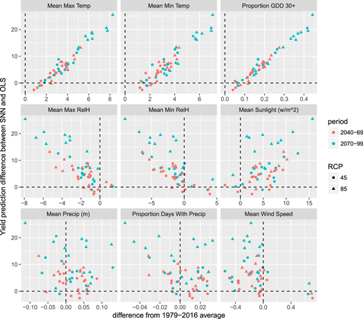
Figure 4. Difference between SNN and OLS projections, plotted against changes between GCMs/scenarios/time periods and 1979–2016 climate.
Download figure:
Standard image High-resolution imageThe spatial distribution of these projections for the Canadian Earth System Model—which is roughly in the middle of projected severity of yield impact, out of our suite of models—is presented in figure 5. While OLS specifications are generally more pessimistic, they project increases in the northernmost regions of our study area. SNN projections do not share this feature, though they are less pessimistic overall. This feature is replicated to varying degrees in all but the most-severe scenarios in other models (see stacks.iop.org/ERL/13/114003/mmedia, which provides corresponding maps for all models). Given that the OLS specification simply measures heat exposure and total precipitation, this suggests that changes besides just increasing heat are likely to inhibit yields.
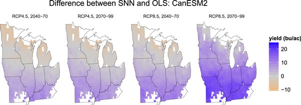
Figure 5. Spatial distribution of difference in yield projections between the semiparametric neural network, and the parametric model for a single member of our climate model ensemble (CanESM2). The OLS regression tends to be more optimistic than the SNN in the northern sections of the study region, and more pessimistic in the southern regions. See supplementary figures for output from other GCMs.
Download figure:
Standard image High-resolution image5. Discussion
On average, yield impacts projected by the neural net—in response to future weather scenarios simulated by global climate models—are somewhat less severe than those projected using parametric models. Nonetheless, these estimates are still among the more severe estimates for temperate-zone corn compared to the studies compiled for the IPCC 5th Assessment Report (Porter et al 2013). It is worth emphasizing that the difference in yield projections between the statistical approaches considered here is not as large as the difference in yield projections between climate models and emissions scenarios.
We find that the timing of heat and moisture are important to predicting corn yields, along with the simple accumulation of heat. This is seen both in the less-pessimistic projections in the south of our study area, and the lack of positive responses to increasing warmth in the north of our study area. As such, we find that GDDs are a useful but imperfect proxy for the role of heat in predicting crop yield. Indeed, work has indicated important roles for VPD and soil moisture (Roberts et al 2012, Lobell et al 2013, Anderson et al 2015, Urban et al 2015) in explaining and building upon the baseline parametric specification. The complexity of these underlying response mechanisms is an argument for the explicit use of GCMs in assessing climate change impacts on agriculture, which explicitly capture the co-evolution of multiple climate variables.
While deep learning has led to substantial breakthroughs in predictive applications and artificial intelligence, classical statistical methods will remain central to scientific applications that seek to elucidate mechanisms governing cause and effect. We describe a semiparametric approach that fuses the two and works better than either alone in terms of predictive performance. This approach is suitable for any prediction problem in which there is some—potentially imperfect—prior knowledge about the functions mapping inputs to outcomes, and longitudinal or other structure in the data.
Ultimately, we find that combining ML with domain-area knowledge from empirical studies improves predictive skill, while altering conclusions about climate change impacts to agriculture. There is substantial scope to refine and extend this work, along four major avenues: (1) better representations of domain-area knowledge in the parameterization of the parametric component of the model, (2) extension to wider geographic areas, which will require more-explicit treatment of differences in seasonality of production over space, (3) bringing the nonparametric (neural network) part of the model closer to the research frontier in ML and artificial intelligence, and (4) finding ways to integrate elements from deterministic crop models that have heretofore been challenging to model statistically, such as CO2 fertilization.
6. Methods
The panelNNET R package (See footnote 2) was used to train SNN used in this analysis. Key features of this package are described below.
6.1. Training Semiparametric Neural Networks
There no closed form solution for a parameter set that minimizes the loss function of a neural network; training is done by gradient descent. This is complicated by the fact that neural nets have many parameters—it is common to build and train networks with more parameters than data. As such, neural networks do not generally have unique solutions, and regularization is essential to arriving at a useful solution—one that predicts well out-of-sample. This section describes basic ways that this is accomplished in the context of semiparametric neural nets.
Our training algorithm seeks a parameter set that minimizes the L2-penalized loss function

where  and λ is a tunable hyperparameter, chosen to make the model predict well out-of-sample. Larger values of λ lead to inflexible fits, while values approaching zero will generally cause overfitting in large networks.
This loss is minimized through gradient descent by backpropagation—an iterative process of computing the gradient of the loss function with respect to the parameters, updating the parameters based on the gradient, recalculating the derived regressors, and repeating until some stopping criterion is met. Computing the gradients involves iterative application of the chain rule:
where '⊙' indicates the elementwise matrix product.
After computing gradients, parameters are updated by simply taking a step of size δ down the gradient:
A challenge in training neural networks is the prevalence of saddle points and plateaus on the loss surface. In response, a number of approaches have been developed to dynamically alter the rate at which each parameter is updated, in order to speed movement along plateaus and away from saddlepoints. We use RMSprop:
where g is the gradient ∂R/∂Γ. Where past gradients were low—perhaps because of a wide plateau in the loss surface—the step size is divided by a very small number, increasing it. See Ruder (2016) for an overview of gradient descent algorithms.
Rather than computing the gradients at each step with the full dataset, it is typically advantageous to do so with small randomized subsets of the data—a technique termed 'minibatch' gradient descent. One set of minibatches comprising the whole of the dataset is termed one 'epoch.' Doing so speeds computation, while introducing noise and thereby helping the optimizer to avoid small local minima in the loss surface.
Another technique used to improve the training of neural networks is 'dropout' (Srivastava et al 2014). This technique randomly drops some proportion of the parameters at each layer, during each iteration of the network, and updates are computed only for the weights that remain. Doing so prevents 'co-adaptation' of parameters in the network—development of strong correlations between derived variables that ultimately reduces their capacity to convey information to subsequent layers.
6.2. The 'OLS trick'
While gradient descent methods generally perform well, they are inexact. The top level of a neural network is a linear model however, in derived regressors in the typical context or in a mixture of derived regressors and parametric terms in our semiparametric context. Ordinary least squares provides a closed-form solution for the parameter vector that minimizes the unpenalized loss function, given a set of derived regressors, while ridge regression provides an equivalent solution for the penalized case.
We begin by noting that the loss function (equation (4)) can be recast as

as such, a given λ implies a 'budget' for deviation from zero within elements of  . After the mth iteration, the top level of the network is

Because gradient descent is inexact, the parameter sub-vector ![$[{\beta }^{m},{{\rm{\Gamma }}}^{m}]\equiv {{\rm{\Psi }}}^{m}$](https://content.cld.iop.org/journals/1748-9326/13/11/114003/revision2/erlaae159ieqn8.gif) does not satisfy
does not satisfy

where ![${\bf{W}}\equiv [X,V]$](https://content.cld.iop.org/journals/1748-9326/13/11/114003/revision2/erlaae159ieqn9.gif) , dm indicates the 'within' transformation for fixed-effects models, and
, dm indicates the 'within' transformation for fixed-effects models, and  is the penalty corresponding to the 'budget' that is 'left over' after accounting for the lower level parameters which generate V. We calculate the implicit
  for the top level of the neural network by minimizing
where
Replacing Ψm with  ensures that the sum of the squared parameters at the top level of the network remains unchanged, but that the (top level of the) penalized loss function reaches its minimum subject to that constraint. We term this the 'OLS trick,' and employ it to speed convergence of the overall network.
6.3. Yield modeling algorithm
A central challenge in training neural networks is choosing appropriate hyperparameters, such that the main parameters constitute a model that predicts well out-of-sample. This is further complicated by the fact that optimal hyperparameters—such as learning rate and batch size—can vary over the course of training. We thus employ combination bayesian hyperparameter optimization (BHO) and early stopping, and form an ensemble of models trained in this fashion—bootstrap aggregation—to further improve performance.
Bootstrap aggregating—or 'bagging'—(Breiman 1996) involves fitting a model to several bootstrap samples of the data, and forming a final prediction as the mean of the predictions of each of the models. Bagging improves performance because averaging reduces variance. Expected out-of-sample predictive performance for each model can be assessed by using the samples not selected into the bootstrap sample as a test set—termed the 'out of bag' sample. Out-of-sample performance for the bagged predictor can be assessed by averaging all out-of-bag predictions, and comparing them to observed outcomes.
BHO seeks to build a function relating test set performance to hyperparameters, and then select hyperparameters to optimize this function. We do so iteratively—beginning with random draws from a distribution of hyperparameters, we fit the model several times using these draws in order to create a joint distribution of hyperparameters and test-set performance. We use this joint distribution to fit a model

where Φ is a matrix of hyperparameters, with rows indexing hyperparameter combinations attempted. 'Improvement' is a vector of corresponding improvements to test-set errors, measured relative to the starting point of a training run. The model  is a random forest (Breiman 2001).
After several initial experiments, we use a numerical optimizer to find
and then fit the SNN with hyperparameters Φnew, generating a new test error and improvement. This is repeated many times, until test error ceases improving.
Early stopping involves assessing test-set performance every few iterations, and exiting gradient descent when test error ceases improving. There is therefore a 'ratcheting' effect—updates that do not improve test error are rejected, while updates that do improve test error serve as starting points for subsequent runs.
We combine these three techniques, performing BHO with early stopping within each bootstrap sample. Specifically, we begin the fitting procedure for each bootstrap sample by selecting a set of hyperparameters that is likely to generate a parameter set  that will overfit the data—driving in-sample error to near-zero (which typically implies a large out-of-sample error).
BHO commences from that starting point, using random draws over a distribution of the following hyperparameters:
- λ—L2 regularization. Drawn from a distribution between [2−8, 25].
- Parametric term penalty modifier. Drawn from a distribution between zero and one. This is a coefficient by which λ is multiplied when regularizing coefficients associated with parametric terms at the top level of the model. Values near zero correspond to an OLS regression in the parametric terms, and values of 1 correspond to a ridge regression. This term does not directly affect parameters relating top-level derived variables to the outcome.
- Starting learning rate—coefficient multiplying the gradient when performing updates. Drawn from a distribution between
![$[{10}^{-6},{10}^{-1}]$](data:image/png;base64,iVBORw0KGgoAAAANSUhEUgAAAAEAAAABCAQAAAC1HAwCAAAAC0lEQVR42mNkYAAAAAYAAjCB0C8AAAAASUVORK5CYII=) .
. - Gravity—after each iteration in which the loss decreases, multiply the learning rate by this factor. Drawn from a distribution between [1, 1.3].
- Learning rate slowing rate—after each iteration in which the loss increases, divide the learning rate by gravity, to the power of the learning rate slowing rate. Drawn from a distribution between [1.1, 3].
- Batchsize—the number of samples on which to perform one iteration. Drawn from a distribution between [10, 500].
- Dropout probability—the probability that a given node will be retained during one iteration. Dropout probability for input variables is equal to dropout probability for hidden units, to the power of 0.321, i.e. if Dropout probability for hidden units is 0.5, then the probability for input variables to be retained is 0.50.321 ≈ 0.8. Drawn from a distribution between [0.3, 1].
![$[{10}^{-6},{10}^{-1}]$](https://content.cld.iop.org/journals/1748-9326/13/11/114003/revision2/erlaae159ieqn15.gif)
Each draw from the hyperparameters is used to guide the training a model, updating  . On every 20th run, the 'OLS trick' is applied to optimize the top-level parameters, and then test set error is measured. Where test error reaches a new minimum, the associated parameter set
  is saved as the new starting point. Where test error fails to improve after 5 checks, training exits and is re-started with a new draw of Φ, after concatenating a new row to be used in training model (6). Given that the optimal set of hyperparameters can change over the course of training, only the most recent 100 rows of
 ![$[\mathrm{Improvement},{\rm{\Phi }}]$](https://content.cld.iop.org/journals/1748-9326/13/11/114003/revision2/erlaae159ieqn18.gif) are used to train model (6).
are used to train model (6).
Finally, we iterate between BHO and random hyperparameter search, in order to ensure that the hyperparameter space is extensively explored, while also focusing on hyperparameter values that are more likely to improve test-set performance. Specifically, a random draw of hyperparameters is performed every third run, followed by two runs using hyperparameters selected to maximize (6).
The above procedure is done for each of 96 bootstrap samples, yielding models that are tuned to optimally predict withheld samples of years. The final predictor is formed by averaging the predictions of each member of the 96-member model ensemble.
Code for conducting BHO—as well as code underpinning the rest of the analysis described here, is available at http://github.com/cranedroesch/ML_yield_climate_ERL.
Data availability
All data used in this study are publicly available. Gridded surface meteorological data are published by the Northwest Knowledge Consortium, and are available at http://thredds.northwestknowledge.net:8080/thredds/reacch_climate_MET_aggregated_catalog.html. Yield and irrigation data are available from the USDA's National Agricultural Statistical Service, and are available at https://nass.usda.gov/Quick_Stats/. CMIP5 runs, downscaled using MACA, are also available from the Northwest Knowledge consortium, at https://climate.northwestknowledge.net/MACA/data_portal.php. Soil data from SSURGO is publicly available at https://gdg.sc.egov.usda.gov/.
Code used to perform this analysis is available at https://github.com/cranedroesch/ML_yield_ERL.