

Abstract
To determine the remaining carbon budget, a new framework was introduced in the Intergovernmental Panel on Climate Change's Special Report on Global Warming of 1.5 °C (SR1.5). We refer to this as a 'segmented' framework because it considers the various components of the carbon budget derivation independently from one another. Whilst implementing this segmented framework, in SR1.5 the assumption was that there is a strictly linear relationship between cumulative CO2 emissions and CO2-induced warming i.e. the TCRE is constant and can be applied to a range of emissions scenarios. Here we test whether such an approach is able to replicate results from model simulations that take the climate system's internal feedbacks and non-linearities into account. Within our modelling framework, following the SR1.5's choices leads to smaller carbon budgets than using simulations with interacting climate components. For 1.5 °C and 2 °C warming targets, the differences are 50 GtCO2 (or 10%) and 260 GtCO2 (or 17%), respectively. However, by relaxing the assumption of strict linearity, we find that this difference can be reduced to around 0 GtCO2 for 1.5 °C of warming and 80 GtCO2 (or 5%) for 2.0 °C of warming (for middle of the range estimates of the carbon cycle and warming response to anthropogenic emissions). We propose an updated implementation of the segmented framework that allows for the consideration of non-linearities between cumulative CO2 emissions and CO2-induced warming.
Export citation and abstract BibTeX RIS

Original content from this work may be used under the terms of the Creative Commons Attribution 4.0 license. Any further distribution of this work must maintain attribution to the author(s) and the title of the work, journal citation and DOI.
1. Introduction
Carbon budgets relate cumulative emissions of carbon dioxide (CO2) to global-mean temperature change. The carbon budget concept gained widespread attention in 2009 (Allen et al 2009, Matthews et al 2009, Meinshausen et al 2009, Zickfeld et al 2009) and ever since a range of scientific literature has assessed and quantified it (recently, e.g. Millar et al (2017), Tokarska and Gillett (2018), Goodwin et al (2018)).
Though conceptually simple, the details of a carbon budget derivation are complex (Rogelj et al 2016). As a metric, the carbon budget combines multiple characteristics of the Earth system's response to anthropogenic emissions into a single number: how much CO2 can be released into the atmosphere without exceeding a given warming threshold. Accordingly, it is sensitive to a number of factors including estimates of the climate system's response to CO2 emissions (Raupach 2013, Collins et al 2013, Gillett et al 2013) and assumptions about the impact of non-CO2 climate forcers (Mengis et al 2018, Simmons and Matthews 2016). While carbon budgets are widely used, recent re-assessments have led to criticism of the concept, in particular for being subject to large uncertainties (Peters 2018).
The IPCC's Special Report on Global Warming of 1.5 °C (SR1.5) introduced a new framework to assess the relationship between warming and cumulative CO2 emissions (Rogelj et al 2018) that was later extended and formalised in Rogelj et al (2019). The new, 'segmented' framework (section 2) separately quantifies the contributions of different climate system components, considering historical warming, CO2-induced warming, warming due to non-CO2 climate drivers, the zero emissions commitment and the impact of otherwise unrepresented processes. These separate assessments are then combined to derive the overall relationship between cumulative CO2 emissions and warming.
The segmented framework has two clear advantages. Firstly, it ensures that assumptions about the importance of different components of the climate system are explicit. Secondly, the assessments of each component are assumed to be independent, hence they can be sourced from specialist research communities and multiple lines of evidence.
The framework's simplicity may also come with disadvantages. The climate system includes feedbacks and interactions between its components, which are explicitly not included in the segmented framework.
In the SR1.5's implementation of the framework, a strictly linear relationship between cumulative CO2 emissions and CO2-induced warming at the time of net zero CO2 emissions was assumed. However, the linear relationship between cumulative CO2 emissions and CO2-induced warming is a first-order approximation (MacDougall 2016). For Earth System Models (ESMs), small deviations from linearity can be seen in Gillett et al (2013). The linear approximation overestimates warming for most models, particularly BNU-ESM, CanESM2 and HadGEM2-ES (note that the y-axis in figure 2(c) of Gillett et al (2013) is relative: for cumulative emissions above 1,000 GtC, residuals as small as 0.1 are absolute deviations of 0.1 °C or more). For some Earth System Models of Intermediate Complexity (EMICs), the deviations from linearity are yet more pronounced (see e.g. MacDougall 2016). Given that errors of this size can change 1.5 °C remaining carbon budget estimates by 200 GtCO2 (∼20%) (Rogelj et al 2018), a linear approximation may not be sufficiently precise for estimating our rapidly dwindling remaining carbon budget. The assumption of strict linearity also implies that the transient climate response to emissions (TCRE) is independent of the rate of emissions. In contrast, previous studies detect a small dependence on the rate of CO2 emissions, particularly at low emissions rates (Krasting et al 2014).
Hence we also examine the results of implementing the segmented framework without the assumption of strict linearity. Our updated implementation allows for a non-linear relationship between cumulative CO2 emissions and CO2-induced warming whilst also providing a direct link to existing methods and metrics.
The study begins by discussing the theoretical background of the segmented framework. We then describe the methods used to quantify our key question i.e. the impact of implementing the segmented framework under the assumption of a strictly linear relationship between cumulative CO2 emissions and CO2-induced warming.
We find that the SR1.5's assumption of strict linearity between cumulative CO2 emissions and CO2-induced warming limits the ability to replicate model simulations which include climate feedbacks and interactions. However this discrepancy can be greatly reduced if the segmented framework is implemented without this assumption.
The paper is structured in the following way. Firstly, we calculate the remaining carbon budget from model simulations which include interactions between the climate system's components (figure 1). This provides a benchmark against which we can test the extent to which different implementations of the segmented framework approximate the non-linear interactions and feedbacks within the climate system. Secondly, we implement the segmented framework following the assumption of strict linearity between CO2 emissions and CO2-induced warming (figure 2) and compare it to our model simulations which include interactions between the climate system's components (figure 3). This is, to our knowledge, the first time the performance of implementations of the segmented framework has been investigated and quantified. Thirdly, we propose a new (weakly non-linear) parameterisation to capture the relationship between cumulative CO2 emissions and CO2-induced warming (figure 4). Fourthly, we demonstrate that implementing the segmented framework with our updated parameterisation results in better agreement with the results from model simulations which include interactions between the climate system's components (figure 5).

Figure 1. Calculating the remaining carbon budget from model simulations with interacting climate components. For each scenario assessed in SR1.5 we diagnose peak warming and compatible cumulative CO2 emissions (section 3.1). (a) Cumulative CO2 emissions; (b) Atmospheric CO2 concentrations; (c) Total, non-CO2 greenhouse gas (GHG) and aerosol radiative forcing; (d) Surface temperature rise; (e) Relationship between surface temperature rise and cumulative CO2 emissions, including a linear regression between peak warming and compatible cumulative CO2 emissions over all scenarios. CO2 emissions from permafrost feedbacks are included in all simulations but are not shown here (see instead Panel (l) of figure 2).
Download figure:
Standard image High-resolution image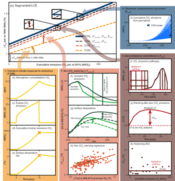
Figure 2. SR1.5-style remaining carbon budget assessment. The assessment uses the segmented framework, implemented with a linear conversion to cumulative CO2 emissions ('segmented-LCE'). (a) Combination of the independent assessments of the climate system's components; (b)-(e) Assessment of the TCRE using a 1pctCO2 experiment; (f)-(h) Assessment of the non-CO2 warming; (i)-(k) Assessment of the zero (CO2) emissions commitment; (l) Assessment of the contribution of processes not considered in the other components (so-called 'otherwise unrepresented processes'). All magnitudes are illustrative only.
Download figure:
Standard image High-resolution image
Figure 3. Relationship between cumulative CO2 emissions (rel. to 2011) and peak surface temperature (rel. to 2006-2015) calculated following the segmented-LCE implementation (red line) and model simulations with interacting climate components (blue dashed line). The grey dots represent the peak warming from each simulation, with one simulation being performed per SR1.5 scenario.
Download figure:
Standard image High-resolution image
Figure 4. Non-linearity in the relationship between CO2-induced warming and cumulative CO2 emissions. Panels (a) and (b) show the relationship on conventional, cumulative CO2 emissions–CO2-induced warming axes. Panels (c) and (d) show the residuals from the assumption of strict linearity, based on the TCRE derived from a 1pctCO2 experiment. Panel (a) shows warming relative to pre-industrial while panel (b) shows warming relative to 2006-2015. Given that the residuals calculated in panels (c) and (d) are derived from panels (a) and (b), respectively, the difference between panels (c) and (d) is due to the different reference periods. The assumption of strict linearity (which is part of the LCE implementation of the segmented framework) is only an approximation of the relationship between CO2-induced warming and cumulative CO2 emissions at the time CO2 emissions reach net zero.
Download figure:
Standard image High-resolution image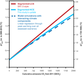
Figure 5. Updated implementation of the segmented framework. The segmented-NCE implementation represents the relationship between CO2-induced warming and cumulative CO2 emissions with a logarithmic fit to CO2-only experiments based on 1.5 °C and 2.0 °C scenarios. As a result, it agrees more closely with the results from model runs with interacting climate components than the segmented-LCE implementation with its assumption of strict linearity.
Download figure:
Standard image High-resolution image
We conclude that the segmented framework's independence assumptions do not introduce any significant error in and of themselves. However, the choices made whilst implementing the framework are important and can introduce unintended inconsistencies. In particular, the non-linearity in the relationship between cumulative CO2 emissions and CO2-induced warming alters remaining carbon budget estimates by around 10%. We recommend that implementations of the segmented framework consider our update in order to capture this effect.
2. Background
The SR1.5 approach can be captured by the following equation (Rogelj et al 2018), Rogelj et al 2019)
where  is the remaining carbon budget,
  is the peak temperature limit,
  is historical, human-induced warming,
  is the contribution of non-CO2 climate forcers to warming or cooling at the time when CO2 emissions reach net zero,
  is the zero emissions commitment (ZEC) i.e. the warming or cooling that emerges after CO2 emissions reach net zero, TCRE is the transient climate response to emissions and
  is a CO2-equivalent emissions term which represents the impact of processes or feedbacks which are not considered in the other components (we refer to these as 'emissions from otherwise unrepresented processes'). All terms are relative to a recent reference period except for
  , which is the temperature target relative to a pre-industrial reference period,
  , which is the warming between the pre-industrial and recent reference periods, and
  , which is the warming after CO2 emissions reach net zero.
Equation (1) can be written in a more general form as
where C is cumulative CO2 emissions at the time CO2 emissions reach net zero (relative to the reference period),  is CO2-induced warming from the reference period onwards at the time CO2 emissions reach net zero and f is a transformation which maps between
  and C. As long as f is a one-to-one mapping, a finite remaining carbon budget can be calculated for arbitrary temperature targets.
Equations (1) and (2) are examples of the 'segmented framework' because they assess the remaining carbon budget via the combination of a number of separate terms. The key assumption of the segmented framework is that each contributing term is independent, i.e. there are no temperature contributions arising from interactions between the different components e.g. there is no temperature contribution from CO2–non-CO2 feedbacks.
However, the total warming we have seen since industrialisation is the result of non-linear interactions and feedbacks, which are not included in the approximation defined in the segmented framework of equation (2). As discussed in section 1, this study is the first attempt to investigate and quantify the implications of using different implementations of the segmented framework. By using a single model throughout our study, we isolate the impact of methodological choices from individual process quantifications.
3. Methods
In this paper, we follow the same convention as SR1.5 and hence use the term 'remaining carbon budget' to refer to the cumulative amount of CO2 that can be released from a given point in time (e.g. 2018) without ever exceeding a peak warming level like e.g. 1.5 °C. It takes all anthropogenic forcers into account e.g. emissions of CO2, methane, nitrous oxides, and aerosols, multiple feedback processes and any warming which may emerge after CO2 emissions reach net zero.
This definition explicitly excludes overshoot and budgets calculated in this way are not temperature exceedance budgets (Rogelj et al 2016). Instead, the carbon budgets considered here are compatible with remaining below the given temperature target for all time, subject to non-CO2 forcers not causing further warming once CO2-induced warming peaks. This condition holds for all the SR1.5 scenarios (Huppmann et al 2019) used in this study. Accordingly, non-CO2 effects are included in the assessment, but the analysis budget do not precisely quantify limits on non-CO2 emissions.
For estimating the remaining carbon budget we use globally averaged surface air temperature as our metric and provide peak temperature estimates relative to the 1720–1800 reference period. We choose this reference period as a proxy for pre-industrial following the work of Hawkins et al (2017), which suggests that this period may be most appropriate because it had very weak anthropogenic radiative forcing and similar natural radiative forcing to today. We also assume the same historical warming of 1.02 °C between 1720–1800 and 2006–2015 in all our calculations. This 1.02 °C is comprised of 0.97 °C between 1850–1900 and 2006–2015 (as used in SR1.5, Allen et al (2018) plus 0.05 °C between 1720–1800 and 1850–1900 (Hawkins et al 2017).
To match the scenarios and reference period used in SR1.5 exactly, remaining carbon budgets are calculated from 2011 onwards, because the SR1.5 scenarios used throughout this study are harmonised such that all emissions are consistent up until 2010 and vary thereafter. This leads to a minor and negligible variation of the baseline period surface temperature average (2006-2015) for each scenario.
For all of our calculations, we use the Model for the Assessment of Greenhouse Gas Induced Climate Change, version 6 (MAGICC6, Meinshausen et al 2011). MAGICC6 is a key scenario assessment tool which is widely used in the IPCC assessment process (IPCC 2014a, IPCC 2014b) and can be run from Python using Pymagicc (Gieseke et al 2018). Its main components are an upwelling-diffusion ocean, a box-model of the carbon cycle, simplified gas cycles of non-CO2 species and a permafrost module which follows Schneider von Deimling et al (2012). We choose MAGICC6 because it incorporates all of the components required to quantify the extent to which the segmented remaining carbon budget assessment framework can approximate non-linear interactions and feedbacks within the climate system. It is also computationally efficient enough to perform the multiple experiments required by this study. MAGICC6's representation of the climate system is highly parameterised hence does not include explicit representations of all the interactions within the climate system, particularly at the regional level. Nonetheless, on a multi-centennial, global-scale, it has been shown to reproduce the temperature response, climate feedbacks and carbon cycle feedbacks from more complex models (Meinshausen et al 2011, Rogelj et al 2014), such as those from the Third Coupled Model Intercomparison Project (CMIP3, Meehl et al 2007), and Fifth Coupled Model Intercomparison Project (CMIP5, Taylor et al 2012).
To examine the sensitivity of our conclusions to the model calibration, we repeat the entire experiment for a range of plausible carbon cycle and ocean responses, described in Meinshausen et al (2011). Each carbon cycle response emulates a different carbon cycle model that participated in the C4MIP experiment (Friedlingstein et al 2006) while the ocean responses emulate different AOGCM models (Meehl et al 2007). We include the MIROC3.2(hires) ocean calibration in the figures but not in our reported ranges because this calibration's zero emissions commitment is a clear outlier.
3.1. Remaining carbon budget when simulating an interactive climate system
We firstly calculate the remaining carbon budget using model simulations which explicitly consider the interactions and feedbacks within the climate system. This calculation provides a benchmark, against which we can test implementations of the segmented framework.
We run MAGICC6 including all of the components considered by the SR1.5 framework i.e. all anthropogenic and natural forcings as well as its permafrost module (figure 1). MAGICC6's CO2 response component is run in an emissions-driven setup including temperature and fertilisation carbon cycle feedbacks while its non-CO2 component is run in a concentration-emissions hybrid mode. In the historical period MAGICC6 has prescribed atmospheric concentrations for non-CO2 greenhouse gases and prescribed optical thickness for aerosols. For the projection period, it is driven by anthropogenic emissions of greenhouse gases and aerosols.
We run each of the scenarios assessed in SR1.5 (Huppmann et al 2019) through this setup. We then derive cumulative CO2 emissions compatible with the peak warming in each scenario (Supplementary section S2). By performing a linear regression between peak warming and compatible cumulative CO2 emissions over all scenarios (using the statsmodels Python package (Seabold and Perktold 2010)), we can determine the remaining carbon budget for any temperature target (figure 1). When making such a calculation, it should be recognised that the results will likely only hold for ambitious mitigation scenarios i.e. scenarios which reach net zero CO2 emissions.
3.2. Implementing the segmented framework
When implementing the segmented framework, decisions must be made about how to quantify every component. In this study, we focus on the impact of differing decisions about the relationship between CO2-induced warming and cumulative CO2 emissions at the time CO2 emissions reach net zero. For all the other components, we use a consistent set of choices throughout the study. These follow the decisions made in SR1.5 as closely as possible and are described in Supplementary section S2. The combination of section 3 and Supplementary section S2 covers all the items on the reporting check-list proposed in Supplementary Text 3 of Rogelj et al (2019).
The first implementation of the segmented framework follows the SR1.5. We refer to this implementation as 'segmented-LCE' because its key assumption is that, for a given total allowable CO2-induced warming, there should be a 'linear conversion to cumulative CO2 emissions (LCE)' i.e. the relationship between CO2-induced warming and cumulative CO2 emissions at the time CO2 emissions reach net zero is linear.
In contrast, the second implementation uses a 'non-linear conversion to cumulative CO2 emissions (NCE)' hence we refer to it as 'segmented-NCE'. This is a novel implementation which allows the relationship between CO2-induced warming and cumulative CO2 emissions at the time of net zero CO2 emissions to be weakly non-linear whilst still providing a direct link to existing metrics of the climate response to CO2 emissions.
It should be noted that the two implementations presented here represent only two of a range of possible implementation choices, and that other choices are possible. Exploring the implications of other choices is an area for future study, beyond the scope of this paper.
The segmented-LCE implementation assumes a linear relationship between CO2-induced warming and cumulative CO2 emissions at the time CO2 emissions reach net zero,

where C is cumulative CO2 emissions at the time CO2 emissions reach net zero (relative to the reference period).
SR1.5's estimate of the TCRE was based on the range from AR5 (Collins et al 2013, Stocker et al 2013), which is itself based on multiple lines of evidence. The canonical way to derive the TCRE from Earth System Models (ESMs) is described in Gillett et al 2013) and their model based results (5%–95% TCRE range of 0.8 – 2.4 °C per TtC) informed the range used in SR1.5 (33-67% range of 0.8 – 2.5 °C per TtC).
In order to fit within our 'single model' methodology, we do not follow the SR1.5's assumed TCRE range exactly. We use the TCRE definition and methodology from Gillett et al (2013), first introduced by Matthews et al (2009) who define the TCRE of a model as the ratio of warming to cumulative CO2 emissions in a simulation with a prescribed 1% per year increase in CO2 (a '1pctCO2' simulation) at the time when CO2 reaches double its pre-industrial concentration. Cumulative CO2 emissions ( ) and warming (
 ) at the point in time when CO2 concentrations double are shown by the crosses in figures 2(d) and (e), respectively. In this study, our default setup has a TCRE of 1.74 °C per TtC and the TCRE ranges from 1.2 – 2.27 °C per TtC over the assessed MAGICC6 calibrations. These MAGICC6 calibrations emulate various ESMs which, as shown in Gillett et al (2013), show a range of slight deviations from a strictly linear relationship between CO2-induced and warming and cumulative CO2 emissions.
The segmented-NCE implementation examines the benefits of considering a non-linear relationship between CO2-induced warming and cumulative CO2 emissions at the time CO2 emissions reach net zero. The first step in this implementation is deciding on a specific form for the non-linear relationship between CO2-induced warming and cumulative CO2 emissions at the time CO2 emissions reach net zero. We motivate this form by considering the counteracting processes which lead to a nearly linear relationship between surface warming and cumulative CO2 emissions. The key balance is between the weakening of carbon sinks as cumulative anthropogenic CO2 emissions increase and the near logarithmic relationship between atmospheric CO2 concentrations and radiative forcing (Matthews et al 2009, MacDougall 2016). Following this, we use a logarithmic relationship (equation (4)). For completeness, we recognise that the balance between weakening carbon sinks and logarithmic CO2 radiative forcing only holds when atmospheric CO2 concentrations are changing. When concentrations are approximately constant, an approximately constant TCRE emerges because the increasing sensitivity of warming to radiative forcing (Ehlert et al 2017) largely balances the decrease in emissions required to keep concentrations constant (due to the weakening carbon sinks). Even though the exact functional form of these cancellations is uncertain, a logarithmic function is sufficient to examine the impact of deviations from linearity in the relationship between cumulative CO2 emissions and CO2-induced warming at the time CO2 emissions reach net zero.
Having chosen a logarithmic formulation, we seek a function which reduces to strict linearity under certain limits.
Here, as previously,  is CO2-induced warming from the reference period onwards at the time CO2 emissions reach net zero and C is cumulative CO2 emissions at the time CO2 emissions reach net zero (relative to the reference period).
  and
and  are, also as previously, defined as the warming and cumulative CO2 emissions, respectively, at the point in time when CO2 concentrations double in a 1pctCO2 experiment. The constants γ and α allow for pathway dependence and non-linearity in the relationship between CO2-induced warming and cumulative CO2 emissions.
To fit the constants α and γ in our framework, we run all the SR1.5 scenarios whose CO2 emissions reach net zero in a CO2-only setup (without the permafrost module to avoid double counting its contribution). We then fit equation (4) to the warming and cumulative CO2 emissions at the time CO2 emissions reach net zero from all the simulations (Supplementary figure S3).
The reason for this choice becomes more evident if we reconsider equation (2). Within equation (2), the conversion between CO2-induced warming and cumulative CO2 emissions need only apply at the time at which CO2 emissions reach net zero. This is a subtle, yet important, point. It means that the conversion between CO2-induced warming and cumulative CO2 emissions does not need to represent the transient relationship between CO2-induced warming and cumulative CO2 emissions over a range of CO2 emissions rates. Instead, it must be applicable to a range of cumulative CO2 emissions but only needs to apply at one CO2 emissions rate, zero. In addition, existing literature (Krasting et al 2014) suggests that the relationship between CO2-induced warming and cumulative CO2 emissions may be rate-dependent, particularly at low emissions rates. Hence care must be taken when applying the results from an experiment in which CO2 emissions do not reach net zero (e.g. the 1pctCO2 experiment) to analyses that do consider net zero scenarios. Our fitting methodology avoids any potential inconsistencies which might arise from assuming that the transient relationship between cumulative CO2 emissions and CO2-induced warming can be directly used to infer the relationship between cumulative CO2 emissions and CO2-induced warming at the time CO2 emissions reach net zero over a range of cumulative CO2 emissions.
We examine equation (4) more closely to explain the choice and effect of the constants in more detail. Under the limit  , equation (4) becomes (via a Taylor expansion)
With  , we recover the segmented-LCE implementation's linear relationship between cumulative CO2 emissions and CO2-induced warming (equation (3)). By further choosing γ = 1, we return to the simplest and most common assumption about the relationship between CO2-induced warming and cumulative CO2 emissions i.e.
  with
with  .
.
Thus, variations in γ scale the relationship between CO2-induced warming and cumulative CO2 emissions to account for departures from the results of the 1pctCO2 experiment.
In contrast, variations in α control how far equation (4) deviates from linearity. For finite values of α, equation (4) is non-linear. If α is positive then the relationship is sub-linear (physically this corresponds to the case where the saturation of CO2 radiative forcing dominates). On the other hand, negative α leads to a super-linear relationship (weakening of carbon sinks dominating). It is important to note that the warming at C = 0 and  are independent of the value of α. The curvature between these two points is controlled by α, however only variations in γ can lead to
  .
.
The smaller α becomes, the greater the deviation from linearity. For example, take  and
and  equal to 2.0 °C and 3 667 GtCO2, respectively i.e. a TCRE of 0.54 °C per TtCO2, equal to the 50th percentile estimate from Rogelj et al (2018). For α = 7334 GtCO2 (
 ), cumulative CO2 emissions compatible with a temperature target of 1.5 °C are approximately 40 GtCO2 bigger and cumulative CO2 emissions compatible with a temperature target of 2.0 °C are approximately 170 GtCO2 bigger than those inferred from a strictly linear relationship with equivalent TCRE (Supplementary section S3, particularly Supplementary table S1).
4. Results and Discussion
We find that the segmented-LCE implementation in our single-model experiment yields notably different results from the actual model simulations (figure 3). For a target peak temperature of 1.5 °C above pre-industrial (represented by the period 1720–1800, (Hawkins et al 2017), the difference in remaining carbon budget estimates is approximately 50 GtCO2 (10%). This difference is slightly larger than the recent emissions uncertainty in table 2 of SR1.5 (20 GtCO2). For a target peak temperature of 2.0 °C above pre-industrial the difference grows and the methods disagree by 260 GtCO2 (17%) (table 1). This difference is a similar size to the non-CO2 scenario variation and historical temperature uncertainties presented in table 2 of SR1.5 (250 GtCO2).
Table 1. Estimates of the remaining carbon budget from 2011 (all estimates have been rounded to the nearest 10 GtCO2). In square brackets we provide the maximum and minimum estimates over all model calibrations (except MIROC3.2(hires), see section 3). The carbon budget ranges marked with a * are those for which, for some MAGICC6 tunings, no scenarios stayed below this temperature target and hence the reported range is an extrapolation of results from the assessed scenarios. For convenience, we also show warming relative to 1850-1900 in parentheses. As this paper only includes results from one model, the absolute carbon budget estimates do not represent full uncertainty ranges.
| Approximate peak surface temperature rel. to 1720–1800 (rel. to 1850–1900 in parentheses) | Model simulations with interacting climate components | Segmented-LCE (linear conversion to cumulative CO2 emissions) | Segmented-NCE (non-linear conversion to cumulative CO2 emissions) | ||
|---|---|---|---|---|---|
| (°C) | Estimate (GtCO2) | Estimate (GtCO2) | Difference from model simulations (GtCO2) | Estimate (GtCO2) | Difference from model simulations (GtCO2) |
| 1.50 (1.45) | 510 (80, 1 190)* | 460 (280, 810) | −50 (−380, 200) | 510 (300, 1 120) | 0 (−180, 220) |
| 1.55 (1.50) | 610 (170, 1 330.0)* | 540 (350, 920) | −70 (−410, 180) | 600 (370, 1 270) | −10 (−170, 200) |
| 1.60 (1.55) | 710 (260, 1 480.0)* | 620 (410, 1 020) | −90 (−460, 160) | 690 (440, 1 430) | −20 (−170, 180) |
| 1.65 (1.60) | 800 (360, 1 630.0)* | 690 (480, 1 120) | −110 (−510, 150) | 770 (510, 1 590) | −30 (−160, 150) |
| 1.70 (1.65) | 900 (450, 1 770) | 770 (540, 1 230) | −130 (−540, 130) | 860 (580, 1 750) | −40 (−150, 130) |
| 1.75 (1.70) | 1000 (540, 1 920) | 850 (610, 1 330) | −150 (−590, 120) | 950 (650, 1 920) | −50 (−140, 110) |
| 1.80 (1.75) | 1100 (640, 2 070) | 920 (670, 1 430) | −180 (−640, 110) | 1040 (730, 2 090) | −60 (−140, 90) |
| 1.85 (1.80) | 1200 (730, 2 210) | 1000 (740, 1 530) | −200 (−680, 90) | 1130 (800, 2 260) | −70 (−130, 70) |
| 1.90 (1.85) | 1290 (820, 2 360) | 1080 (800, 1 640) | −210 (−720, 80) | 1230 (870, 2 440) | −60 (−120, 80) |
| 1.95 (1.90) | 1390 (910, 2 510) | 1150 (870, 1 740) | −240 (−770, 70) | 1320 (940, 2 620) | −70 (−120, 110) |
| 2.00 (1.95) | 1490 (990, 2 650) | 1230 (930, 1 840) | −260 (−810, 60) | 1410 (1010, 2 800) | −80 (−120, 150) |
| 2.05 (2.00) | 1590 (1080, 2 800) | 1310 (1000, 1 950) | −280 (−850, 40) | 1510 (1080, 2 990) | −80 (−130, 190) |
| 2.10 (2.05) | 1680 (1160, 2 950) | 1380 (1060, 2 060) | −300 (−900, 40) | 1600 (1150, 3 180) | −80 (−130, 230) |
| 2.15 (2.10) | 1780 (1250, 3 090) | 1460 (1130, 2 160) | −320 (−940, 20) | 1700 (1220, 3 380) | −80 (−130, 290) |
| 2.20 (2.15) | 1880 (1330, 3 240) | 1540 (1190, 2 270) | −340 (−990, 10) | 1800 (1300, 3 580) | −80 (−140, 340) |
| 2.25 (2.20) | 1980 (1420, 3 390) | 1620 (1260, 2 370) | −360 (−1030, 0) | 1890 (1370, 3 780) | −90 (−140, 390) |
| 2.30 (2.25) | 2070 (1500, 3 530) | 1690 (1320, 2 480) | −380 (−1070, −10) | 1990 (1440, 3 990) | −80 (−140, 460) |
| 2.35 (2.30) | 2170 (1590, 3 680) | 1770 (1390, 2 580) | −400 (−1120, −30) | 2090 (1510, 4 200) | −80 (−130, 520) |
| 2.40 (2.35) | 2270 (1680, 3 830) | 1850 (1450, 2 690) | −420 (−1160, −30) | 2190 (1590, 4 420) | −80 (−140, 590) |
| 2.45 (2.40) | 2370 (1760, 3 970) | 1920 (1520, 2 800) | −450 (−1200, −50) | 2290 (1660, 4 640) | −80 (−140, 670) |
| 2.50 (2.45) | 2470 (1850, 4 120) | 2000 (1580, 2 900) | −470 (−1250, −50) | 2390 (1730, 4 860) | −80 (−140, 740) |
| Root-mean square error | N/A | N/A | 290 (40, 850) | N/A | 70 (50, 330) |
Table 2. Breakdown of the differences between the segmented-LCE and segmented-NCE implementations of the segmented framework by component for selected peak warming targets ( ).
).  is historical warming,
  is the zero-emissions commitment,
  is warming due to non-CO2 climate drivers at the time when CO2 emissions reach net zero relative to the reference period,
  is warming due to CO2 emissions,
  is the implied TCRE, C is total cumulative CO2 emissions,
  is cumulative emissions from otherwise unrepresented processes in 2100 and
  is total cumulative anthropogenic CO2 emissions i.e. the remaining carbon budget. The driver of differences between the two frameworks is the relationship between cumulative CO2 emissions and CO2-induced warming, which is captured by the implied TCRE. Values in parentheses show min-max ranges over all model calibrations which were used in this study (except MIROC3.2(hires) which was labelled as an outlier). Accordingly, these ranges do not illustrate scenario related uncertainties. Additionally, as this study only includes results from one model the shown ranges do not represent the full uncertainty.
 (rel. to 1720–1800) (°C) (rel. to 1720–1800) (°C) |
Component | Segmented-LCE | Segmented-NCE |
|---|---|---|---|
| 1.5 |  (°C) (°C) |
1.02 | 1.02 |
 (°C) (°C) |
0.01 (0.01, 0.03) | 0.01 (0.01, 0.03) | |
 (°C) (°C) |
0.22 (0.19, 0.25) | 0.22 (0.19, 0.25) | |
 (°C) (°C) |
0.24 (0.21, 0.28) | 0.24 (0.21, 0.28) | |
| C (GtCO2) | 520 (400, 830) | 560 (400, 1130) | |
(Implied)  (°C / TtCO2) (°C / TtCO2) |
0.47 (0.33, 0.62) | 0.43 (0.25, 0.59) | |
 (GtCO2) (GtCO2) |
50 (20, 110) | 50 (20, 110) | |
 (GtCO2) (GtCO2) |
460 (280, 810) | 510 (300, 1120) | |
| 2.0 |  (°C) (°C) |
1.02 | 1.02 |
 (°C) (°C) |
0.01 (0.01, 0.03) | 0.01 (0.01, 0.03) | |
 (°C) (°C) |
0.36 (0.29, 0.4) | 0.36 (0.29, 0.4) | |
 (°C) (°C) |
0.61 (0.56, 0.68) | 0.61 (0.56, 0.68) | |
| C (GtCO2) | 1280 (1050, 1860) | 1470 (1090, 2820) | |
(Implied)  (°C / TtCO2) (°C / TtCO2) |
0.47 (0.33, 0.62) | 0.41 (0.22, 0.57) | |
 (GtCO2) (GtCO2) |
50 (20, 110) | 50 (20, 110) | |
 (GtCO2) (GtCO2) |
1230 (930, 1840) | 1410 (1010, 2800) |
Allowing for non-linearity in the relationship between cumulative CO2 emissions and CO2-induced warming, as in the segmented-NCE implementation, significantly reduces this difference (figure 5). The difference between remaining carbon budget estimates based on the segmented-NCE implementation and estimates based on model simulations with interacting climate components is around 0 GtCO2 for 1.5 °C of warming and only 80 GtCO2 (5%) for 2.0 °C of warming.
The non-zero y-intercept of the solid lines in figure 5 implies that, under the assumptions of the segmented framework, if we were to stop emitting immediately, we would still see a temperature rise of approximately 0.2 °C. This is because of the non-CO2 contribution, ZEC and emissions from otherwise unrepresented processes, all of which are assessed to be non-zero even if CO2 emissions cease immediately. However, given that the components of the segmented framework have not been assessed under such immediate cessation scenarios, it should also not be used to make conclusions about 'locked-in' warming. If the segmented framework were to be used to assess warming for such rapid emissions reductions then the assessment of these components should be reconsidered.
Compared to the segmented-LCE implementation, the segmented-NCE implementation better captures the relationship between cumulative CO2 emissions and CO2-induced warming. The improvement becomes particularly pronounced when we are interested in warming and cumulative emissions from a recent reference period, rather than pre-industrial (figures 4(a) and (b)).
There are two causes of this improved representation. The first is that, as previously discussed, the relationship between cumulative CO2 emissions and CO2-induced warming is weakly non-linear. This is the case in the explored MAGICC6 calibrations as well as the models they are emulating (see figure 2 of Gillett et al (2013) and figure 2(c) of MacDougall (2016)). This is reflected in the results of the 1pctCO2 experiment (figure 4, specifically the difference between the orange dashed line and the solid gray line in figure 4(c)). Fitting equation (4) to the transient relationship between warming and cumulative CO2 emissions from the 1pctCO2 experiment (with γ = 1 to ensure that our fit passes through the TCRE), we find α = 8094 GtCO2 (red dashed lines in figure 4). For our default setup, this results in  (given
  GtCO2, Supplementary table S3) and hence deviations from linearity of order 100 GtCO2 (Supplementary table S1).
The second reason for our improved representation of the relationship between cumulative CO2 emissions and CO2-induced warming is that we fit to the warming and cumulative CO2 emissions at the time CO2 emissions reach net zero from scenario based experiments. This change in fitting dataset allows us to capture the difference between two subtly different relationships: (1) the transient relationship between CO2 warming and cumulative CO2 emissions and (2) the relationship between CO2 warming and cumulative CO2 emissions at the time CO2 emissions reach net zero. This difference is highlighted in figure 4, specifically the difference between the red dashed line and the blue dashed line in figure 4(c). As discussed in section 3.2, this difference may arise because we focus on warming at the time of net zero CO2 emissions and the climate's response to CO2 emissions depends on the CO2 emissions rate itself (Krasting et al 2014). We find a fitted value of γ = 0.94 i.e. we must scale the results of the 1pctCO2 experiment down by 6% in order to match the results from 1.5 °C and 2.0 °C scenarios.
We find that there is a discrepancy between the peak warming—cumulative CO2 emissions relationship diagnosed from the segmented-LCE implementation and the relationship derived from the segmented-NCE implementation for all model calibrations (Supplementary figures S4 and S5). However, the discrepancy is not uniform, with both the linearity and scaling of results from the 1pctCO2 experiment varying amongst the different model calibrations (Supplementary table S3). We find a weak correlation where calibrations whose ocean heat uptake efficiency declines more (less) strongly in response to warming have more (less) linear responses i.e. larger (smaller) α. Although examining the physical drivers of non-linearity in detail is beyond the scope of this paper, at first consideration this appears to agree with our previous reasoning. A decline in ocean heat uptake efficiency will increase the sensitivity of warming to radiative forcing, leading to greater cancellation with the approximately logarithmic CO2 radiative forcing and hence a more linear response.
In most cases, we find that using the segmented-NCE implementation, rather than the segmented-LCE implementation, results in noticeably smaller deviations from the results of model simulations with interacting climate components (Supplementary figures S6 and S7). The exception is for peak temperature limits above 2.0 °C relative to pre-industrial. Given that our study focuses on ambitious mitigation scenarios, we have low confidence that either of the segmented implementations really represents the dynamics of the system at higher warming targets where feedbacks become more important. In the interests of scope, we leave further exploration for future study.
Given the improved performance of the segmented-NCE implementation across a wide range of carbon cycle and ocean responses, we feel that there is a clear need to allow for a non-linear relationship between cumulative CO2 emissions and CO2-induced warming within remaining carbon budget assessment. Under the segmented-LCE implementation it is not possible to consider a non-linear relationship and hence its effect might be missed.
Given the range of possible implementations of the segmented framework, we suggest a small adjustment to the reporting suggested by Rogelj et al (2019). We suggest reporting remaining carbon budget assessments in the style of table 2, where the implied TCRE can itself vary with the peak warming target. This provides greater flexibility for remaining carbon budget assessment studies without reducing the ability to compare their conclusions. In contrast, we do not recommend attempting to summarise results within a single equation because this may not always be possible and can quickly obscure the contributions of the different climate components (Supplementary section S4).
At this point the strengths of the segmented framework are clear. In particular, it facilitates comparison of differences between remaining carbon budget estimates (e.g. table 2 makes clear that the only difference between the segmented-LCE implementation and the segmented-NCE implementation is the treatment of CO2). On the other hand, our linear regression based on model simulations with interacting climate components alone simply results in the relationship  °C / TtCO2 ×C + 0.22 °C (R-squared = 0.98, Supplementary table S2). From this, no information about the breakdown of contributions from each climatic component can be inferred, hindering easy diagnosis of differences from other estimates.
5. Limitations
The results presented here come with a number of limitations that call for future research beyond this study. To start with, we have analysed implementations of the segmented framework in only one way. While our analysis is able to identify one key area for improvement, other approaches may identify other weaknesses, for example those that may currently be hidden because of compensating errors.
Secondly, determining α and γ using exactly the same methodology as this study cannot practically be done with ESMs because of the large number of simulations required. The segmented framework allows problems like this to be overcome because it combines multiple lines of evidence. This is most obvious in the inclusion of otherwise unrepresented processes, which ensures that the processes which are currently not assessed by ESMs are nonetheless considered. We feel that the segmented-NCE implementation follows exactly the same logic. The starting point could still be strict linearity ( , γ = 1), based on the TCRE from ESMs. This could be extended with estimates of α from ESMs' existing 1pctCO2 simulations. Then other lines of evidence, such as well-calibrated emulators or observations (although disentangling estimates of the different components e.g. the contribution of CO2 separate from non-CO2 factors would certainly be a challenge), can further inform the magnitude of the non-linearity and scenario dependence in the relationship between CO2-induced warming and cumulative CO2 emissions at the time CO2 emissions reach net zero. Equation (4) can then be used to combine multiple lines of evidence, utilising their respective strengths and ensuring that the impact of non-linearity and scenario dependence in the relationship between CO2-induced warming and cumulative CO2 emissions is included in remaining carbon budget assessment.
Thirdly, we have not considered how uncertainty in the overall remaining carbon budget can be quantified. As acknowledged in SR1.5 (Rogelj et al 2018), the segmented framework provides no way to formally combine all the relevant uncertainties into an overall uncertainty. This is because the components and their uncertainties are assessed and combined independently. In contrast, model simulations with interacting climate components could be extended to quantify uncertainty by using a probabilistic parameter set of the kind developed by Meinshausen et al (2009). By sampling a range of plausible climate responses, a probability density function for the carbon budget as a function of peak warming could be determined. We do not attempt such an assessment here as there are no formally derived, up-to-date distributions available and developing one is beyond the scope of this paper. Nonetheless, in the area of uncertainties, model simulations with interacting climate components offer a more obvious way forward than the segmented framework.
Fourthly, non-CO2 assessment and related uncertainties have not been discussed in any detail. Problems are immediately evident in the low R-squared values seen in the regression between non-CO2 warming and warming at the time of net zero CO2 emissions (Supplementary section S2 and Supplementary table S2). Reconsidering how the non-CO2 contribution is assessed within the segmented framework is an obvious area for further examination.
Finally, it is still not clear how land-use change CO2 emissions should be included. As Simmons and Matthews (2016) note, there is little research into whether the climate response to land-use change CO2 emissions might differ from the climate response to fossil CO2 emissions (as one directly changes the size of the global land carbon pool whilst the other does not). The lack of a clear protocol about whether diagnosis experiments should include land-use change emissions or not is a problem for clarity, consistency and comparability.
6. Conclusions
We have found that the non-linearity and pathway dependence of the relationship between CO2-induced warming and cumulative CO2 emissions at the time of net zero CO2 emissions may have a non-negligible impact on remaining carbon budget estimates. As a result, we have presented an updated implementation of the segmented remaining carbon budget assessment framework. This update allows researchers to assess the impact of non-linearity and pathway dependence. The impact, which we estimate is approximately 10% of the budget (50 GtCO2 for a 1.5 °C target and 200 GtCO2 for a 2.0 °C target), is larger than the uncertainty associated with recent emissions (±20 GtCO2) and slightly smaller than the uncertainty associated with the TCRE distribution (±200 GtCO2), historical warming (±250 GtCO2) and non-CO2 scenario variation (±250 GtCO2) reported in table 2 of SR1.5 (Rogelj et al 2018). The importance of these effects depends on the dynamics of the climate system hence is subject to some uncertainty. Our update allows this uncertainty to be fully explored.
The non-linearity and pathway dependence of the relationship between peak warming and cumulative CO2 emissions also presents a definitional and communication challenge. At the moment, the TCRE refers both to a single point from the 1pctCO2 experiment (Matthews et al 2009, Gillett et al 2013) and the 'transient surface temperature change per unit cumulative CO2 emissions' (Matthews 2018) i.e. some measure of the gradient of the transient relationship between CO2-induced surface temperature change and cumulative CO2 emissions. We have found that confusing these two meanings can lead to a difference in remaining carbon budget estimates. In addition, our study and existing research (MacDougall 2016, Gillett et al 2013) suggest that the second concept is only approximately constant and hence may not be as useful as the first, which is constant by definition. Addressing these differing definitions would help avoid confusion and facilitate clearer communication within the scientific community and beyond.
The remaining carbon budget for different warming thresholds will remain a key question as we assess the action required to mitigate further anthropogenic climate change. The segmented framework provides an explicit, transparent, intuitive way to combine independent assessments of the different processes which affect the remaining carbon budget. The use of such a framework, in particular for reporting results, makes the assumptions underlying remaining carbon budget estimates explicit and clear. Nonetheless, the implementation choices made when using such a framework must be carefully considered. The implementation we have presented here allows for greater flexibility in the representation of the relationship between cumulative CO2 emissions and CO2-induced warming at the time CO2 emissions reach net zero, hence better reproduces the results from analyses which explicitly consider the feedbacks and interactions within the climate system at this critical point in time.
Acknowledgment
We could not have produced this manuscript without the feedback of Sonya Fiddes, Matthias Mengel and David Karoly.
ZN and MM would also like to thank all the participants at the International Workshop on the Remaining Carbon Budget, organised with the support of the Global Carbon Project, the CRESCENDO project, Stanford University, the University of Melbourne, and Simon Fraser University, for the insightful discussions, in particular Joeri Rogelj and Damon Matthews.
We would also like to thank two anonymous reviewers for their careful, detailed and insightful reviews. The manuscript was greatly improved thanks to their efforts and feedback.
Funding
ZN benefited from support provided by the ARC Centre of Excellence for Climate Extremes (CE170 100 023).
Author Contributions
ZN, RG, AN and MM designed the study. ZN, RG, and JL performed the study. ZN and MM designed and produced all the figures. ZN wrote the first draft of the manuscript. All authors contributed to the editing and revisions of the manuscript.
Competing Interests
The authors declare no competing interests.
Data and Materials Availability
The data that support the findings of this study are openly available at https://doi.org/10.5281/zenodo.3726578 and at https://gitlab.com/znicholls/remaining-carbon-budget-frameworks-2020. Pymagicc v2.0.0-beta, which includes MAGICC6, is archived at https://doi.org/10.528 1/zenodo.3386 579.