


Abstract
The impact of winter atmospheric blocking over the Ural Mountains region (UB) coincident with different phases of the North Atlantic Oscillation (NAO) on the sea ice variability over the Barents and Kara Seas (BKS) in winter is investigated. It is found that the UB in conjunction with the positive phase of the NAO (NAO+) leads to the strongest sea ice decline. During this phase composites and trajectory analyses reveal an efficient moisture pathway to the BKS from the mid-latitude North Atlantic near the Gulf Stream Extension region where water vapor is abundant due to high sea surface temperatures. The NAO+-UB combination is an optimal circulation pattern that significantly increases the BKS water vapor that plays a major role in the BKS warming and sea ice reduction, while the increased sensible and latent heat fluxes play secondary roles. By contrast, much fewer dramatic impacts on the BKS are observed when the UB coincides with the neutral or negative phases of the NAO.
Our results present new insights into the complex processes involved with Arctic sea ice reduction and warming. The mechanisms highlighted here potentially offer a perspective into the mechanisms behind Arctic multi-decadal climate variability.
Export citation and abstract BibTeX RIS

Original content from this work may be used under the terms of the Creative Commons Attribution 3.0 licence.
Any further distribution of this work must maintain attribution to the author(s) and the title of the work, journal citation and DOI.
1. Introduction
In recent decades, accelerated Arctic warming and dramatic sea ice decline have been detected (Comiso 2006, Screen and Simmonds 2010, Walsh 2014, Simmonds 2015). This warming has been referred to as the Arctic amplification (AA) because the Arctic has warmed at about twice the global rate over the past half century (Serreze et al 2007, Budikova 2009, Screen and Simmonds 2013, Walsh 2014). While significant progress on identifying the cause of the Arctic warming has been made in the past few years (Screen and Simmonds 2010, Walsh 2014), the relative importance of the myriad of potential physical mechanisms responsible for Arctic warming or AA is still much debated. There is evidence to indicate a two-way interaction between the Arctic warming and mid-latitude weather patterns. In particular Arctic warming may affect middle latitude weather patterns by weakening the west-to-east tropospheric winds (Newson 1973, Murray and Simmonds 1995, Budikova 2009, Overland and Wang 2010, Overland et al 2011, Francis and Vavrus 2012, 2015), while the Arctic region may be affected by variations in middle latitude circulation patterns (Fang and Wallace 1994, Deser et al 2000, Sorteberg and Kvingedal 2006, Frankignoul et al 2014, Park et al 2015). The understanding of these couplings is made all the more difficult because we are dealing with a complicated nonlinear system (Semenov and Latif 2015, Overland et al 2016).
The recent investigations of Luo et al (2016a) and Gong and Luo (2017) have demonstrated that atmospheric blocking over the Ural Mountains of western Russia can amplify Arctic warming and sea ice decline over the Barents and Kara Seas (BKS). This finding is of importance partly because the BKS is an important region of the Arctic for influencing the midlatitudes (Luo et al 2016a, Overland 2016, Yang et al 2016). In addition, Luo et al (2016a) showed by a regression analysis that the atmospheric response to BKS ice decline has a large-scale circulation pattern resembling Ural blocking (UB), superimposed on the positive phase of the North Atlantic Oscillation (NAO+), and that the UB lags the NAO+ by about 4–7 days (Luo et al 2016b). However, whether the combined UB and NAO+ pattern is an optimum circulation that leads to the sea ice decline over the BKS or, conversely, whether the Arctic sea ice decline leads to such a circulation pattern is not clear. In particular, one might ask how the UB with a different phase of the NAO affects the sea ice variability over the BKS.
In this paper, we explore the relationships between UB, phases of the NAO, and BKS sea ice in winter, and propose a new viewpoint that the UB with NAO+ is a circulation pattern which strongly facilitates sea ice decline over the BKS through enhanced moisture intrusion, increases in the downward infrared radiation and warming over the BKS. Our analysis will make use of synoptic analyses to reveal the source of this excess moisture.
2. Data and method
We use daily winter (from December to February, DJF) data from the ERA-interim (ERAI) dataset on a 1° × 1° grid (Dee et al 2011) from December 1979 to February 2016 (1979–2015 hereafter), which includes sea ice concentration (SIC), 500 hPa geopotential height (Z500), surface air temperature (SAT), downward infrared radiation (IR), vertically integrated moisture flux convergence and total column water vapor (TCWV) and sea surface temperature (SST). Here, we use the ERAI SIC data partly because it is internally consistent with the ERAI meteorological fields and is time continuous. We also point out that it is in very close agreement with the satellite SIC data of the National Snow and Ice Data Center (NSIDC) (Park et al 2015).
The daily NAO index is obtained by projecting the daily 500 hPa geopotential height poleward of 20°N onto the loading pattern of the rotated empirical orthogonal functions for the NAO, which is taken from the NOAA /Climate Prediction Center (www.cpc.noaa.gov/products/precip/CWlink/pna/nao.shtml). The daily data has also been deseasonalized and linearly detrended.
To identify blocking events in the Ural region around 60°E (Diao et al 2006), we used the one-dimensional (1D) blocking index of Tibaldi and Molteni (1990, TM hereafter) based on the meridional gradient values of 500 hPa geopotential height Z500:  and
and  for given three latitudes ϕN = 80°N+Δ, ϕ0 = 60°N + Δ and ϕS = 40° N + Δ at a given longitude (λ); and Δ = −5°, 0°, 5° were used here. A blocking event is defined to have taken place in a given region if both GHGS > 0 and (2) GHGN < −10 gpm deg−1 latitude as a TM criterion, with a 5° × 5° longitude-latitude covering area, are satisfied for at least one choice of Δ and persist at least three consecutive days. The blocking is regarded as the UB if it occurs in the region (40°–80°E). Because the TM index is required to satisfy the above conditions for at least three consecutive days, the duration of a UB is at least 3 days and has a typical timescale of two weeks (10–20 d) (Luo et al 2016a). Although the days of a blocking event that satisfies the TM criterion is not identical to its duration (Diao et al 2006), we may refer the TM index-identified days to as the TM duration of a blocking event.
A NAO+ event is defined to have taken place if the daily NAO index has values in excess of 0.5 standard deviations (STDs) above its mean and persists for at least three consecutive days. A NAO− event is defined in an analogous manner with values less than 0.5 STDs below its mean. All other NAO events are referred to as neutral NAO events (NAO°). The life cycle of a NAO+ event is defined to start when the daily NAO index from its first positive anomaly, continues to its peak (which will be ≥ 0.5 STD), and then returns to its first negative anomaly. The persistence time of this life cycle is defined to be the period of the NAO event. Here, we define the day that the GHGS is largest as the lag 0 day. Thus, the UB event is defined to be 'related' to an NAO event if the peak of the GHGS occurs within the life cycle of that NAO event.
For a composite field we use a two-sided student t-test to test its statistical significance when the number of the samples is large enough to fit a normal distribution. Moreover, the Monte-Carlo testing method is used to test the statistical significance of the difference of the domain-averaged time series between two kinds of events by performing 10 000 random experiments.
In our analysis we use an efficient and accurate two-dimensional Lagrangian trajectory tracking method (de Vries and Döös 2001) applied to the vertically integrated water vapor as explained below. The scheme was originally designed for oceanic application (Blanke and Raynaud 1997), but has been applied successfully to tracking atmospheric moisture (e.g. Hua et al 2017).
3. Analyses and results
Over the period 1979–2015 we have identified 54 winter UB events, of which 26 are related to NAO+ events, 8 to NAO− events, and 20 to NAO° events with mean durations of 7.61, 7.30 and 7.85 d, respectively. There are 77 NAO+ events and 34 NAO− events without a UB. Thus, the downstream blocking such as the UB is modulated by the phase of the NAO (Luo et al 2007) and is associated with the North Atlantic jet (Luo et al 2016b). Luo et al (2016b) also found that most of UB events are associated with the NAO+ and the UB lags the NAO+ by 4–7 d. Below, we perform composite analyses in terms of these UB and NAO events to examine why the UB-induced warming and BKS sea ice change depend on the phase of the NAO and whether the NAO without UB leads to the BKS sea ice decline.
Before exploring the ways in which UB-induced warming depends on the phase of the NAO, it is informative to show the spatial structures of time-mean 500 hPa geopotential height and SAT anomalies averaged over a mature period from lag −5 to 5 days of each UB event (lag 0 denotes the day of the maximum GHGS in the daily TM index and is referred to as the maximum TM index day) in figures 1 (a) and (c) for the three cases of UBs with NAO+, NAO− and NAO°, respectively. The BKS warming is greatest when the UB occurs together with the NAO+ (figure 1 (a)), even though the UB strength is slightly less for NAO+ (contour lines in figure 1(a)) than for both the NAO− (figure 1(b)) and NAO° (figure 1(c)). However, the BKS warming is weakest when the UB occurs together with the NAO− (figure 1(b)) but, as opposed to the two other cases, there is significant warming over northeast North America and Greenland. We also see that the BKS warming is less for the UB with NAO° (figure 1(c)) than for the UB with NAO+, and there is little evidence of warming in the NAO− case. In figure 1(d), the negative (positive) lags indicate that the maximum TM index lags (leads) the UB. Thus, this figure clearly shows that the UB starts at about lag −10 days and the maximum amplitude of the UB with NAO+ lags the maximum TM index by about 1 d, whereas the UB with NAO− (NAO°) leads the maximum TM index by about 1 day. In the composite daily field, the UB lags the NAO+ by about 4 days (not shown). It is also found that although the UB with NAO° has a greater duration and a slightly larger amplitude than those of the UB with NAO+ (figure 1(d)) and the UB with NAO− has the almost same amplitude as that with NAO+, the UB-NAO+-related warming is strongest in the three blocking types. These results make clear that the BKS temperature response to UB strongly depends on the concurrent phase of the NAO. Below we explore in detail the physical reasons for this and, in particular, examine the anomalous moisture transports into the BKS in the three phases and the consequences of these for downward IR, sensible and latent heat flux anomalies. The calculation of the shortwave radiation is not presented because the shortwave radiation almost vanishes in winter (Serreze et al 2007). We will then investigate the implications of these processes for BKS SAT and sea ice.

Figure 1 Time-mean (a), (b), (c)) 500-hPa geopotential height and surface air temperature (SAT) (plotted from north of 20°N) anomalies averaged over the mature period from lag −5 to +5 days for Ural blocking (UB) events associated with (a) NAO+, (b) NAO− and (c) NAO° events; and (d) time series of the area-averaged composite daily geopotential height (HGT) anomalies over the region (50°–70°E, 60°−70°N) as the blocking amplitudes for UB events with NAO+ (blue line), NAO− (red line) and NAO° (neutral NAO) (yellow line). Lag 0 denotes the maximum GHGS day of the daily TM index and the green box denotes the BKS region. In following figures, lag 0 and the green box have the same meanings. In panels (a)–(c), only regions above the 95% confidence level for a two-sided Student's t-test are shaded. The gray shading denotes the difference of the HGT between the NAO+ and NAO− has a 95% confidence level for a Monte-Carlo test. Negative (positive) lags indicate that the maximum TM index lags (leads) the other variable.
Download figure:
Standard image High-resolution imageThe time-mean SIC anomalies averaged from lag −5 to 5 days are shown in figures 2 (a) and (c) for UBs with NAO+, NAO− and NAO°. We can see that for the UB with NAO+ the SIC anomaly is negative over the BKS and weakly positive over the Labrador Sea (figure 2(a)). But a reversed SIC anomaly pattern with a prominent sea ice decline (rise) over the Labrador Sea (BKS) is seen for the UB with NAO− (figure 2(b)). For the UB with NAO°, it seems that the sea ice decline is found mainly over the BKS (figure 2(c)). Thus, the sea ice variability over the Labrador Sea is likely directly related to the phase of the NAO, consistent with previous findings (Deser et al 2000, Strong et al 2009, Frankignoul et al 2014). However, as noted below, while the NAO+ has no effect on the BKS sea ice when the UB is absent, the NAO− has an effect onto the BKS sea ice and leads to an increase of the SIC in the BKS. Thus, the above result suggests that the UBs with different phases of the NAO can lead to different variations of the sea ice between the BKS and Labrador Sea. This is likely related to the different distributions of the moisture and associated downward IR for the UBs with different phases of the NAO.

Figure 2 Time-mean (a), (b), (c)) sea ice concentration (SIC) anomalies (plotted from north of 60°N) averaged over the mature period from lag −5 to +5 days for Ural blocking (UB) events associated with (a) NAO+, (b) NAO− and (c) NAO° events; and ((d), (e)) time series of the area-averaged (d) SAT and (e) SIC anomalies over the Barents and Kara Seas (BKS, 30°–80°E, 65°–80°N) for UB events with NAO+ (blue line), NAO− (red line) and NAO° (yellow line) events. In panels ((a), (c)), only regions above the 95% confidence level for a two-sided student t-test are shaded. The time interval between two vertical solid lines denotes the life cycle of the composite UB identified by the TM index from lag −10 to 10 d, whereas the interval between two vertical dashed lines represents the time average range of the mature period for the UB. In panel days (e), the gray shading denotes that the difference of the SAT (SIC) between the NAO+ and NAO− has a 95% confidence level for a Monte-Carlo test.
Download figure:
Standard image High-resolution imageFigure 2(d) shows that during the time interval from lag −20 to −10 days the SAT anomaly averaged over the BKS (taken here to be the box 30°–80°E, 65°–80°N) is positive and slightly larger for the UB with NAO− and NAO° than that with NAO+. A statistical significance test shows that their difference is not significant. After lag −10 day, the BKS warming or positive SAT anomaly tends to strengthen (weakens) as the UB intensifies (decays) for all phases of the NAO. For the UB with NAO+ and NAO° the SAT (figure 2(d)) shows an in-phase variation with the UB amplitude (figure 1(d)) except for a 1 day delay of the SAT for the UB with NAO−. Thus, it is concluded that the enhanced BKS warming is attributed to the intensified UB. However, the UB-NAO+-related BKS warming (blue line in figure 2(d)) is more intense and persistent than those with the NAO− and NAO°, although the amplitude (duration) of the UB with NAO+ is not largest (longest) (figure 1 (d)). This motivates us to infer that over the BKS the stronger warming is related to more water vapor import for the UB with NAO+ than those with NAO− and NAO°. As we will see below, the water vapor variability over the BKS is closely related to the UB with different phases of the NAO (figure 2 (f)).
Turning to the sea ice (figure 2(e)), the decline is strongest for the UB with the NAO+ (blue line) because the BKS warming is strongest (blue line in figure 2(d)), and the sea ice reaches its decline peak at lag +5. Thus, the sea ice decline (figure 2(e)) lags the UB peak (figure 1 (d)) by about 4 days for the UB with NAO+ because the UB amplitude reaches its peak at lag 1 day. This result also holds for the other two types of blocking. Although the decline of the UB-induced BKS ice is weaker for the NAO° (yellow line in figure 2 (e)), it is much stronger than that for the NAO− (red line in figure 2(e)). Our results show, similar to those for SAT, that the BKS sea ice response depends on the UB on a two-week (10–20 days) timescale and also critically on the phase of the NAO.
To investigate why the BKS warming is different for the three UB-NAO combinations, in figure 3 we show the time-mean fields of composite daily downward IR, TCWV, evaporation and vertically integrated moisture flux convergence anomalies averaged from lag −5 to 5 days for the UBs with NAO+, NAO− and NAO° events. It is found that for the UB with NAO+ the downward IR is strongest in the three types of blocking (figure 3(a)), less strong for the UB with NAO° (figure 3(c)), and only marginally positive for the NAO− case (figure 3(b)). As pointed out in previous studies (e.g. Kapsch et al 2013, Woods et al 2013, Woods and Caballero 2016), the amount of water vapor is crucial for the strength of downward IR. Figures 3(d) and (f)) show that the spatial distribution of the TCWV anomalies are highly consistent with those of downward IR. Accordingly, for the UB with NAO+ the TCWV in the BKS region is largest (figure 3(d)), followed by that of the UB with NAO° case (figure 3 (f)), and with the UB-NAO− combination (figure 3(e)) exhibiting only a very modest increase. Boisvert and Stroeve (2015) and Burt et al (2016) noted that a moistening of the Arctic atmosphere is associated, in part, with increased evaporation from the newly ice-free regions. However, Park et al (2015) also indicated that the evaporation is unimportant for the warming in the BKS. Instead the increased water vapor from midlatitude is most important for the warming (Woods et al 2013, Park et al 2015, Woods and Caballero 2016). While the evaporation over the BKS is greater for the UB with NAO+ (figure 3(g)) than the other two types of blocking (figures 3(h) and (i)), further analysis below shows that the role of the latent heat flux related to the evaporation in the BKS warming is secondary. Thus, in this paper we will focus on examining where the BKS water vapor comes mainly from, rather than making a detailed comparison of the contributions from the moisture intrusion and evaporation. Below, we demonstrate that the flux of moisture from midlatitudes, particularly in the UB –NAO+ combination, is a key component over moisture variability over the BKS.
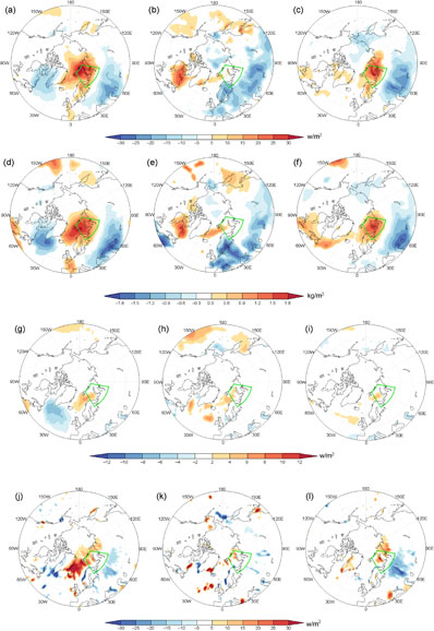
Figure 3 Time-mean (a), (b), (c)) downward IR, (d), (e), (f)) total column water vapor and (g), (h), (i)) evaporation multiplied by 28.5 (1 mm day−1 = 28.5 W m−2) and (j), (k), (l)) moisture flux convergence anomalies (plotted from north of 40°N) averaged from lag −5 to 5 days around lag 0 day for the UB with the NAO+ (left; (a), (d), (g), (j)), NAO− (middle; (b), (e), (h), (k)) and NAO° (right; (c), (f), (i), (l)). Only regions above the 95% confidence level for a two-sided Student's t-test are shaded in panels (a)–(l).
Download figure:
Standard image High-resolution imageThe reasons for the very large amounts of precipitable water over the BKS for the UB with NAO+ case can be explained, in part, in terms of the time-mean fields of the composite daily moisture flux convergence anomalies averaged from lag −5 to 5 days in figure 3(j). It is interesting to see that a strong positive moisture flux convergence anomaly appears on the upstream side (from the east of Greenland to the Norwegian Sea) of the BKS for the UB with NAO+ (figure 3(j)). This implies that the moisture intrusion into the BKS is enhanced through the Norwegian Sea (figure 3(d)). This can be confirmed by calculating the BKS-averaged moisture flux convergence anomaly time series (figure 4 below). The high DJF-mean BKS moisture flux convergence corresponds to less sea ice extent in the BKS (not shown), and vice versa. We also see in figures 3(k) and (l) that the moisture flux convergence over the region upstream of the BKS is weak for two cases of the UB with NAO− (figure 3(k)) and NAO° (figure 3(l)), especially for UB with NAO− (figure 3(k)). Thus, the increased water vapor is smaller over the BKS for the UB with NAO−. Although the moisture flux convergence anomaly is weak for the UB with NAO°, the water vapor has larger values over the BKS compared with those for the NAO−. This implies that for the UB with NAO° the increase in moisture over the BKS also comes from the UB-induced moisture transport from midlatitudes. Thus, it appears that for the UB with NAO+ the moisture intrusion to the BKS contributes more to the increase of the BKS water vapor than do other sources. In closing we comment that the time-mean fields show that the downward IR is in correspondence with the TCWV and moisture flux convergence, it is difficult to use these time-mean fields to nail down the causal relationship between the UB and downward IR or water vapor.
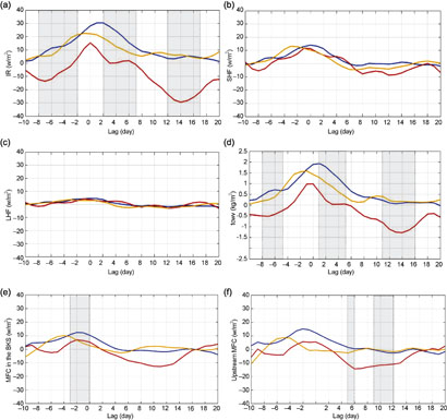
Figure 4 Time series of composite daily (a) downward IR, (b) sensible heat flux (SHF), (c) latent heat flux (LHF) and (d) total column water vapor (TCWV) anomalies averaged over the BKS and (e), (f) composite daily vertically integrated moisture flux convergence (MFC) (multiplied by the latent heat of vaporization L = 2.26 × 10⁶ m2s−2) anomalies averaged in the BKS and upstream BKS region (0°–30°E, 65°–80°N), defined as the MFC in the BKS (e) and upstream MFC (f) respectively, for the UB with NAO+ (blue line), NAO− (red line) and NAO° (yellow line) events. The gray shading denotes that the difference of the downward IR or TCWV or MFC between the NAO+ and NAO− has a 95% confidence level for a Monte-Carlo test.
Download figure:
Standard image High-resolution imageTo cast further light on the relationships revealed in figure 3 and the importance of water vapor over the BKS, it is insightful to show the time evolution of the composite daily TCWV, downward IR, sensible heat flux (SHF), latent heat flux (LHF) and moisture flux convergence (MFC) anomalies averaged over the BKS in figures 4(a) and (e) and the upstream MFC anomaly averaged over the region (00–30°E, 65°–80°N) in figure 4(f) for the three UB-NAO combinations. It is seen that the variations of the downward IR, water vapor, SHF and LHF, and especially the first two, tend to be in phase with the growth and decay of the UB. In particular, the structures of the time series of TCWV (figure 3(d)) and downward IR (figure 3(a)) anomalies show a striking degree of similarity. The TCWV (figure 4(d)) has positive correlations of 0.51, 0.53, and 0.51 with the downward IR (figure 4(a)) for the UBs with NAO+, NAO− and NAO°, respectively (all statistically significant at the 95% confidence level for the student t-test). It is also found that while the SHF (figure 4(b)) is obviously larger than the LHF (figure 4(c)) for the UB-NAO+ combination, it is secondary compared to the role of the intensified downward IR (figure 4(a)) related to increased BKS water vapor (figure 4(d)). Such increased BKS water vapor is related to the intensified moisture flux convergence in the Norwegian Sea (figure 4(f)) and in the BKS region (figure 4(e)) due to the presence of the UB. In figures 4(e) and (f), the fact that the differences in the moisture flux convergence between the NAO+ and NAO− are less significant in some time intervals may be due to noisier fields of the moisture flux convergence. Albeit so, the above results reveal that large increases in water vapor and downward IR over the BKS require that the UB and NAO+ must be combined.
To distinguish the different roles of the UB and NAO and compare with the above results, we show the time-mean composite daily Z500, SAT, TCWV and SIC anomalies averaged from lag −5 to 5 days in figures 5(a) and (f) for the NAO+ and NAO− without UB. For the NAO+ (figure 5 (a)) a warming (cooling) is found over Eurasia (Greenland), while there are cold anomalies over north Eurasia and North America and a warm anomaly over Greenland for the NAO− (figure 5(b)) (Hurrell et al 2003). As further shown by figures 5(c) and (d), in the BKS region there is less water vapor for the NAO+ (figure 5(c)) and a negative water vapor anomaly for the NAO− that is statistically significant (blue shading in figure 5(d)) when the UB is absent, although the largest negative TCWV anomaly is located in the southwest side of the BKS. Especially for the NAO+, the moisture cannot enter the BKS region, instead it can intrude into mid-latitude Eurasia (figure 5(c)) when the UB disappears. As a result, more sea ice (statistically significant at the 95% level), can be seen over the BKS for the NAO+ (figure 5(e)) and NAO− (figure 5(f)) due to reduced downward IR related to decreased water vapor, while the BKS sea ice increase is stronger for the NAO− than for the NAO+. This can also be seen from the BKS-averaged SIC time series as shown in figure 5(g). These results show that the NAO− and even the NAO+ are unable to result in sea ice decline over the BKS if the UB is not present, thus indicating that the combined UB and NAO+ patterns are much more important for the sea ice decline over the BKS (figure 2(e)) than either of the UB and NAO+ alone.
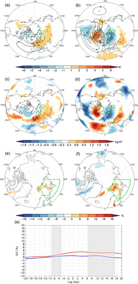
Figure 5 (a), (b) Time-mean 500-hPa geopotential height (contour) and SAT (color), (c), (d) total column water vapor (TCWV) (plotted from north of 20°N) and (e), (f) SIC (plotted from north of 60°N) anomalies averaged from lag −5 to 5 days of (a) NAO+ (77 cases) and (b) NAO− (34 cases) events without concurrent blocking and (g) the corresponding time series of composite daily SIC anomaly averaged over the BKS for the NAO+ (blue) and NAO− (red) events during 1979–2015. Lag 0 denotes the peak day of the NAO. Only regions above the 95% confidence level for a two-sided student t-test are shaded in panels (a), (f). In panel (g), the gray shading denotes that the difference of the SIC between the NAO+ and NAO− has a 95% confidence level for a Monte-Carlo test.
Download figure:
Standard image High-resolution imageAn insightful and novel way to understand the important synoptic physics behind these associations and the import of moisture into the Arctic is to diagnose the source regions of that moisture (Simmonds et al 1999). We undertake this in the next subsection using a parcel trajectory approach. To reveal the source regions for this water vapor we use the version of the two-dimensional Lagrangian trajectory tracking method of de Vries and Döös (2001) to determine the origin region of vertically-integrated water vapor intruding into the BKS for our cases of UB with the different phases of the NAO. This tracking algorithm is applied in an inverse (or 'back trajectory') manner, and hence identifies the origin points of atmospheric parcels arriving some days later at a specific point (in our case, locations within the BKS) (Hua et al 2017).
Figure 6 shows the trajectories of moisture intruding into the BKS for the three categories of UB events in terms of the two dimensional moisture-weighted horizontal velocity. The moisture trajectories in the plots are traced in the time-inverse sequence from lag 0 to lag −10 d. The starting points of the back trajectories are in the BKS where the grid points in the BKS are marked by the red box. For convenience, 49 spaced grid points in the region (longitude range from 30.5 to 79.5 and latitude range from 65.5 to 79.5) in which the value of every 10 longitude grid point interval for each one latitude point are outputted when the land points have been excluded are used to represent the BKS region. That is to say, there are 49 trajectories for each 10 day moisture tracing. The color of the trajectory indicates the column precipitable water at the starting point (i.e. at a grid point in the BKS) and, in particular, a red trajectory indicates that the air at that point in the BKS has high moisture content. There are many such red trajectory lines located in the midlatitude North Atlantic for the UB-NAO+ combination (figure 6(a)). This is because in the NAO+ more eastward migrating cyclones are found in the North Atlantic midlatitudes, and these carry more heat and moisture than their counterparts to the north. These systems are then deflected northward on the east side of the North Atlantic and this northward deflection is enhanced as the UB intensifies, and more water vapor is directed into the BKS. The increased water vapor is accompanied by a large flux of intensified synoptic cyclones into the BKS due to the modulation of the NAO+ (Simmonds et al 2008). Hence one can see that circulations associated with UB and NAO+ act cooperatively to moisten and warm the air over the BKS because more water vapor comes from the North Atlantic midlatitudes near the Gulf Stream Extension (GSE) for the NAO+ (figure 6(d)) than for the NAO− (figure 6(e)). By contrast for UB with the NAO− the origin points are further to the north (and hence cooler and drier) (figure 6(b)) because there are fewer cyclones in the North Atlantic under the modulation of NAO− (Simmonds et al 2008). The water vapor coming from the mid-latitude North Atlantic is less evident (figure 6(b)) because the North Atlantic cyclone belt or storm track is weakened due to its splitting into two branches that move poleward and equatorward around the upstream side of the Greenland anticyclone as the NAO− occurs (Luo et al 2007, Simmonds et al 2008). Thus, for this case the water vapor does not come from the North Atlantic due to reduced North Atlantic cyclone activity. For the UB with NAO°, part of water vapor over the BKS comes from the midlatitude North Atlantic (figure 6(c)) because the Greenland anticyclone is very weak, although it is less so than that for the UB with the NAO+. This can also be clearly seen from figure 6(e). The above results clearly demonstrate from a synoptic point of view that there is a strong coupling between the BKS ice decline or warming and the UB-NAO+ circulation pattern. In other words, the combined UB and NAO+ patterns results in a cooperative circulation pattern conducive to strong decline of BKS ice through strong BKS warming due to strong downward IR associated with increased water vapor.

Figure 6 10 day Lagragian trajectories of moisture for the three categories of the UB with (a) NAO+; (b) NAO− and (c) NAO°; and (d), (e) the trajectories of moisture with a magnitude equal to or greater than 8 mm day−1 for the UB with (d) NAO+ and (e) NAO°. For the same condition as in panels (d), (e), no trajectory can be seen for the UB with the NAO−. Each moisture trajectory in the plot is traced in reverse chronological order to the 10th day (lag −10 days) before lag 0 of the UB event, and originates from the BKS that is marked by red box. The color of the trajectory represents the magnitude of the vertical integral of water vapor at the starting point in the BKS.
Download figure:
Standard image High-resolution imageWe commented above that many UB-NAO+ trajectories come from the warmer and moister midlatitudes. An interesting additional, and reinforcing, aspect of this is apparent when we show the DJF-mean SST, TCWV and evaporation anomalies for 12 NAO+ and 11 NAO− winters selected according to the ±0.5 STDs of the normalized detrended DJF-mean NAO index during 1979–2015 (figure 7). Here, a NAO+ (NAO−) winter is defined if the detrended DJF-mean NAO index reaches +0.5 (−0.5) STD or more. It is seen that the NAO+ winter has large SST anomalies over the midlatitude North Atlantic near the GSE (figure 7(a)). As noted by Czaja and Frankignoul (2002), Deser et al (2010) and Gastineau and Frankignoul (2015) the NAO has an imprint on the SST in the North Atlantic midlatitudes on interannual and decadal timescales and the NAO+ can correspond to high SST near the GSE region due to the wind stress forcing (Czaja and Frankignoul 2002). An interesting result we find here is that the high SST anomaly can intrude into the BKS for the NAO+ winter (figure 7(a)) likely through an oceanic heat advection (Ärthun et al 2012) and the wind-forced positive Atlantic water temperature anomalies over the Nordic Seas and Barents Sea (Schlichtholz and Houssais 2011) probably because of the southwesterlies in the eastern North Atlantic associated with the NAO+. This is not apparent in the NAO− winter (figure 7(b)). The water vapor amount over the BKS in the NAO+ winter (figure 7(c)) exceeds that of the NAO− winter (figure 7(d)). But an evaporation anomaly is almost invisible over the BKS for the NAO+ (figure 7(e)) and NAO− (figure 7(f)) winters, even though the BKS SST is warmer. This indicates that during the NAO+ winter the increases in moisture over the BKS originate predominantly from the moisture intrusion from mid-latitudes, rather than from the evaporation. Also note that the region of large positive SST anomalies over the western North Atlantic near the GSE in NAO+ winters exhibits strong positive anomalies of TCWV (figure 7(c)) and evaporation (figure 7(e)) as these are related to the high SST (Stephens 1990), while the more modest SST anomalies in the NAO− corresponds to negative anomalies of TCWV (figure 7(d)) and evaporation (figure 7(f)). It follows that during the NAO+ winter the mid-latitude North Atlantic south of the GSE, in association with the very strong mean winds experienced in this region (Simmonds and Keay 2002), can provide a ready source of water vapor. This process serves to reinforce the efficient UB -NAO+ transport mechanisms discussed above.
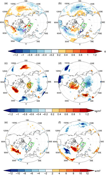
Figure 7 Composite DJF-mean (a), (b) SST, (c), (d) TCWV and (e), (f) evaporation anomalies multiplied by 28.5 (1 mm d−1 = 28.5 W m−2) for 12 NAO+ (a), (c), (e)) and 11 NAO− (b), (d), (f)) winters during 1979–2015, in which the green box denotes the BKS. In panels (a), (b), the area encompassed the purple line denotes the region above the 95% confidence level for a two-sided t-test. Only regions above the 95% confidence level for a two-sided Student's t-test are shaded in panels (c), (f).
Download figure:
Standard image High-resolution imageWe point out that, in accord with the above results, a number of studies have highlighted the Gulf Stream region as an important influence on variability over the BKS. For example, Sato et al (2014) made use the wave-activity flux approach to identify a stationary Rossby wave teleconnection pattern due to heating (positive SST anomaly) which originated in the Gulf Stream region and had anomalies over the Barents Sea and Eurasia, while Simmonds and Govekar (2014) came to a similar conclusion using the very different approach of Rossby wave source identification.
4. Conclusion and discussions
In this paper, we have examined the combined impact of Ural blocking (UB) and different phases of the NAO on the BKS temperature and ice variability to provide an explanation for why the combination of UB and NAO+ is a most favorable circulation pattern for the BKS warming or sea ice decline. The analysis here reveals that with this combination there is more water vapor over the BKS, with the opposite occurring during UB-NAO− events. More moisture intrusion into the BKS is seen to result in enhanced downward IR and, in turn, stronger warming, while the sensible and latent heat fluxes play only a secondary role for the BKS warming.
A key finding is that the UB together with the NAO+ is the most conducive combination to moisture intrusion into the BKS via the relay associated with the NAO+-UB. Our Lagrangian trajectory analysis reveals that more moisture is transported from the midlatitude North Atlantic during the NAO+ phase because of greater North Atlantic cyclone activity (Simmonds et al 2008) and also because of the very large values of the TCWV near the GSE, the latter being associated with strong positive SST anomalies in that region (figure 7(a)). We have explained that when a NAO+ pattern occurs, the moist air originating from the upstream side of the midlatitude North Atlantic near the GSE migrates eastward (figure 5(c)) because the mid-latitude North Atlantic westerly wind is intensified. The moist air cannot continue its eastward movement once a UB appears, but instead deflects northward in the northeast Atlantic and over the European continent, and then enters the BKS region (figure 3 (d)). This can be clearly seen from figure 6(d). We refer this process to as the NAO+-UB relay mechanism of moisture intrusion because the UB lags the NAO+ when they are combined, as described in figure 8 in the form of a schematic diagram. In this figure, the eastward movement of cyclones or air parcels in the North Atlantic due to the NAO+ and their northward movement in the upstream side of the European continent owing to the UB combine to result in a strong moisture flux convergence in the upstream region of the BKS near the Norwegian Sea. This process transports more water vapor to the BKS and in turn results in a strong increase in downward IR. For the UB with the NAO− the intrusion of moisture into the BKS is much less because of the suppressive role of the Greenland anticyclone of the NAO− upstream. Our result also reveals that for the UB with NAO+ the increase in moisture over the BKS comes mainly from the moisture intrusion through the UB-NAO+ relay rather than from the evaporation. Thus, the above result indicates that the phase of the NAO controls the origin regions of UB-related moisture intrusion over the BKS (figure 7(c)).

Figure 8 Schematic diagram of the enhanced transport of moisture from the water vapor pool in the mid-latitude North Atlantic near the GSE to the BKS through the relay of the NAO+ and UB patterns. The solid red box denotes a water vapor pool over the mid-latitude North Atlantic, the arrow denotes the flow direction and 'H' ('L') represents the anticyclonic (cyclonic) circulation. The large blue dot box denotes a region including Europe and some parts of Asia.
Download figure:
Standard image High-resolution image
Our analysis has focused on the effects of the conjunction of UB events and various phases of the NAO. An interesting issue that arises from our investigation relates to the potential causes of multi-decadal variability in Arctic sea ice and temperature (Polyakov et al 2003, Kinnard et al 2011). It is known that the NAO and North Atlantic midlatitude SST are influenced by the Atlantic Multidecadal Oscillation (Chylek et al 2009, Olafsdottir et al 2013, Gastineau and Frankignoul 2015). This connection raises a very strong possibility of explaining multidecadal sea ice variations via the approach we have taken here. We are now exploring this very important area of research.
The authors acknowledge the support from the National Science Foundation of China (Grant numbers: 41430533 and 41375067). Simmonds was supported by Australian Research Council grant DP160101997.