

Abstract
In order to assess future sea level rise and its societal impacts, we need to study climate change pathways combined with different scenarios of socioeconomic development. Here, we present sea level rise (SLR) projections for the Shared Socioeconomic Pathway (SSP) storylines and different year-2100 radiative forcing targets (FTs). Future SLR is estimated with a comprehensive SLR emulator that accounts for Antarctic rapid discharge from hydrofracturing and ice cliff instability. Across all baseline scenario realizations (no dedicated climate mitigation), we find 2100 median SLR relative to 1986–2005 of 89 cm (likely range: 57–130 cm) for SSP1, 105 cm (73–150 cm) for SSP2, 105 cm (75–147 cm) for SSP3, 93 cm (63–133 cm) for SSP4, and 132 cm (95–189 cm) for SSP5. The 2100 sea level responses for combined SSP-FT scenarios are dominated by the mitigation targets and yield median estimates of 52 cm (34–75 cm) for FT 2.6 Wm−2, 62 cm (40–96 cm) for FT 3.4 Wm−2, 75 cm (47–113 cm) for FT 4.5 Wm−2, and 91 cm (61–132 cm) for FT 6.0 Wm−2. Average 2081–2100 annual SLR rates are 5 mm yr−1 and 19 mm yr−1 for FT 2.6 Wm−2 and the baseline scenarios, respectively. Our model setup allows linking scenario-specific emission and socioeconomic indicators to projected SLR. We find that 2100 median SSP SLR projections could be limited to around 50 cm if 2050 cumulative CO2 emissions since pre-industrial stay below 850 GtC, with a global coal phase-out nearly completed by that time. For SSP mitigation scenarios, a 2050 carbon price of 100 US$2005 tCO2−1 would correspond to a median 2100 SLR of around 65 cm. Our results confirm that rapid and early emission reductions are essential for limiting 2100 SLR.
Export citation and abstract BibTeX RIS

Original content from this work may be used under the terms of the Creative Commons Attribution 3.0 licence.
Any further distribution of this work must maintain attribution to the author(s) and the title of the work, journal citation and DOI.
Introduction
Future sea level rise (SLR) threatens coastal regions around the globe, putting at risk their populations, ecosystems, infrastructure, as well as important other economic and environmental assets (Nicholls 2011, Hallegatte et al 2013, Hinkel et al 2014, Wong et al 2014, Muis et al 2017). As such, the assessment of future SLR impacts poses challenges to many research disciplines, from estimating the geophysical SLR response to climate perturbations and emission pathways on different timescales to assessing regional vulnerabilities as well as adaptation options for communities at risk. With the Shared Socioeconomic Pathways (SSPs), the climate research community has been provided with a new framework that can better address the complex challenges of SLR assessments. The SSP framework combines societal storylines with physical radiative forcing pathways, following up on the initial work of the Representative Concentration Pathways (RCPs) (Moss et al 2010, Van Vuuren et al 2011). The SSP framework will also be the basis for the Scenario Model Intercomparison Project (ScenarioMIP) (O'Neill et al 2016) of Phase 6 of the Coupled Model Intercomparison Project (CMIP6) (Eyring et al 2016).
Five SSPs have been designed to comprehensively capture varying levels of socioeconomic challenges to mitigation and adaptation (O'Neill et al 2017): SSP1 sketches a sustainable pathway, with low challenges to mitigation and adaptation; SSP2 describes the 'middle of the road' trajectory with medium challenges to mitigation and adaptation; SSP3 reflects a future world of regional rivalry with high challenges to both mitigation and adaptation; SSP4 represents a future marked by inequality, with low challenges to mitigation and high challenges to adaptation; and the SSP5 trajectory is dominated by ongoing fossil-fuel development and high energy demand, with high challenges to mitigation and low challenges to adaptation. For each SSP, climate policy effectiveness and adoption is also varied as defined by so-called shared climate policy assumptions (SPAs) (Riahi et al 2017). Under SSPs with low mitigation challenges (SSP1, SSP4), an early adoption of stringent climate policies is assumed. Climate policy adoption is projected to be less effective in the near term in SSP2 and SSP5, while SSP3 is the most pessimistic scenario with regards to climate policy. SSP realizations without any dedicated climate mitigation policies form the so-called SSP baseline scenarios. Depending on the individual SSP characteristics and specific SPAs, mitigation pathways for the energy, industry and land-use sectors are derived to reach the radiative forcing targets (FTs) 6.0 Wm−2, 4.5 Wm−2, 3.4 Wm−2, and 2.6 Wm−2 (Riahi et al 2017). All but the FT 3.4 target have corresponding RCPs (Meinshausen et al 2011a, van Vuuren et al 2011). The SSP5 baseline scenarios can be used as analogues to RCP8.5 realizations, as they show comparable emission pathways and 2100 radiative forcing (Kriegler et al 2017). The current set of SSP scenarios provides several pathways that yield median 2100 GMT increases of 2 °C or less relative to pre-industrial times, mainly under FT 2.6 (Kriegler et al 2014, Riahi et al 2015, Kriegler et al 2017). The set does not provide median pathways that comply with the objective to limit warming to 1.5 °C in the long-term. This more ambitious temperature target was included in the Paris Agreement as an aspirational goal, which could significantly reduce climate change impacts (Schleussner et al 2016). It has been suggested that meeting the 1.5 °C objective would require 2100 radiative forcing values to be closer to 2.0 Wm−2 (Rogelj et al 2015).
Generally, future SLR is a powerful indicator to visualize climate change impacts on a global scale (Steinacher et al 2013). Recent progress in process understanding on Antarctic ice sheet dynamics suggests that SLR projections may have to be corrected upwards (DeConto and Pollard 2016). Additional rapid discharge from the Antarctic ice sheet through hydrofracturing and ice cliff failure could cause significantly more SLR by the end of the 21st century than presented in the Fifth Assessment (AR5) of the IPCC (Church et al 2013). Studies that have included these additional Antarctic discharge processes project 2100 central values under RCP8.5 that are up to one meter higher than the AR5 estimates (Bars et al 2017, Bakker et al 2017a, Wong et al 2017a). Here, we present global mean SLR projections that account for the additional rapid discharge contribution from Antarctica using a new physically-motivated emulator. As such, this study provides markedly higher SLR projections than IPCC AR5. We focus on median and 'likely' 66% model ranges associated with the 2100 SSP SLR projections. We do not assess SLR outcomes for the low probability tails of the projected distributions nor do we attempt to incorporate deep uncertainties in our estimates (Bakker et al 2017b).
The SSP-FT framework allows us to not only analyze future SLR under a wide variety of societal developments but to also clearly distinguish between SLR projections for the non-mitigation baseline scenarios and scenario sets with varying levels of climate mitigation efforts. With the study at hand, we highlight SSP scenario-specific SLR characteristics and assess the role of selected underlying emission and socioeconomic indicators for global mean SLR in 2100.
Methods
SSP details are available via the public SSP database (https://tntcat.iiasa.ac.at/SspDb/) hosted by the International Institute for Applied Systems Analysis (IIASA). Global and regional projections are provided for greenhouse gas (GHG) emissions, energy mix, climate and land cover, demographic and socioeconomic parameters like population growth, gross domestic product (GDP), and consumption. The five SSPs have all or in part been implemented by the IMAGE, MESSAGE, AIM, GCAM, REMIND, and WITCH Integrated Assessment Model (IAM) groups (Bosetti et al 2006, Calvin et al 2017, Fricko et al 2017, Fujimori et al 2017, Kriegler et al 2017, Van Vuuren et al 2017). The SSP scenarios are defined until the year 2100. So-called marker scenarios have been proposed as the main representatives of the underlying respective socioeconomic storylines. These marker scenarios are derived by one IAM for each SSP. The non-marker scenarios are complementary realizations of each SSP storyline by the remaining IAMs. For both marker and non-marker realizations, individual SSPs are provided for the baseline, FT 2.6, FT 3.4, FT 4.5, and FT 6.0 cases described in the introduction. The resulting 105 quantified SSP scenarios are available from the SSP database and were used to force our climate and sea level model. By also using the non-marker scenarios for each SSP, we are able to cover parts of the IAM structural uncertainties underlying the individual pathways. For consistency, all SSP GHG emissions have been harmonized to 2010 RCP8.5 emission levels. Post-2100 extension pathways, as provided for the RCPs by Meinshausen et al (2011a), have not been defined yet. Please see the legend of figures 3 or 4 for the full list of SSP scenarios.
In order to translate the full suite of SSP GHG emission data into a global climate and sea level signal, we apply the recently developed comprehensive sea level emulator by Nauels et al (2017), which is directly coupled to the simple climate carbon-cycle model MAGICC version 6 (Meinshausen et al 2011b). The sea level emulator is part of a group of simplified approaches that resolve the main sea level components (Kopp et al 2014, Mengel et al 2016, Wong et al 2017b). It is calibrated with IPCC AR5 consistent process-based SLR projections and provides global mean SLR estimates based on all major climate-driven contributions including thermal expansion, global glacier mass changes, and the surface mass balance and solid ice discharge of the Greenland and Antarctic ice sheets, as well as the non-climate-driven land water storage contribution. We have updated the Antarctic ice sheet (AIS) solid ice discharge (SID) component of the MAGICC sea level model to cover higher Antarctic sensitivity through hydrofracturing and subsequent ice cliff instability that substantially increases future SLR projections (DeConto and Pollard 2016). We present an AIS SID parameterization with a slow discharge term that depends quadratically on the global mean temperature deviation from a reference temperature and a fast discharge term that can be triggered by passing a threshold temperature. The parameterization is calibrated against AIS discharge projections provided by DeConto and Pollard (2016) that run from the year 1950–2500. The four free parameters are optimized by together minimizing the residual sum of squares under three RCP scenarios for which calibration data was available (RCP8.5, RCP4.5, RCP2.6). Please see the supplementary information available at stacks.iop.org/ERL/12/114002/mmedia for more details on the parameterization and calibration. Our main results incorporate SLR contributions based on the revised AIS SID parametrization, while the IPCC AR5 consistent SLR analysis using the original Nauels et al (2017) design is provided in the supplementary information for comparison. SLR projections are presented relative to 1986–2005 levels throughout the manuscript.
For the projections, we have generated a probabilistic ensemble of 600 runs for every scenario with historically constrained parameter sets applying a Metropolis–Hastings Markov chain Monte Carlo approach (Meinshausen et al 2009). The parameter ensemble also reflects the IPCC AR5 equilibrium climate sensitivity estimates (Rogelj et al 2012, Rogelj et al 2014). The probabilistic modeling framework consistently covers model and climate related uncertainties. For our projections, we follow the IPCC guidelines by adopting a likely range that reflects the 66%–100% probability of an outcome (Mastrandrea et al 2011).
In order to facilitate the interpretation of the SSP SLR projections and to allow for a direct comparison to the RCP scenarios, we have also pooled the scenarios according to their FTs. Like this, we can clearly separate the effects of different climate mitigation levels from the effects of socioeconomic uncertainty in the non-mitigation baseline scenarios. Additionally, we have grouped the 2100 median SLR estimates of each SSP scenario according to individually defined categories for the SSP indicators shown in figures 3 and 4. The category ranges are chosen based on the scenario distribution for the individual SSP indicator. This visual aid is introduced to allow for a more nuanced analysis of the SLR implications of the selected SSP emission and socioeconomic indicators. We use boxplots with 90% range whiskers, the standard first and third quartiles (50% range) as boxes and the corresponding medians for the grouping of the individual 2100 SSP SLR medians.

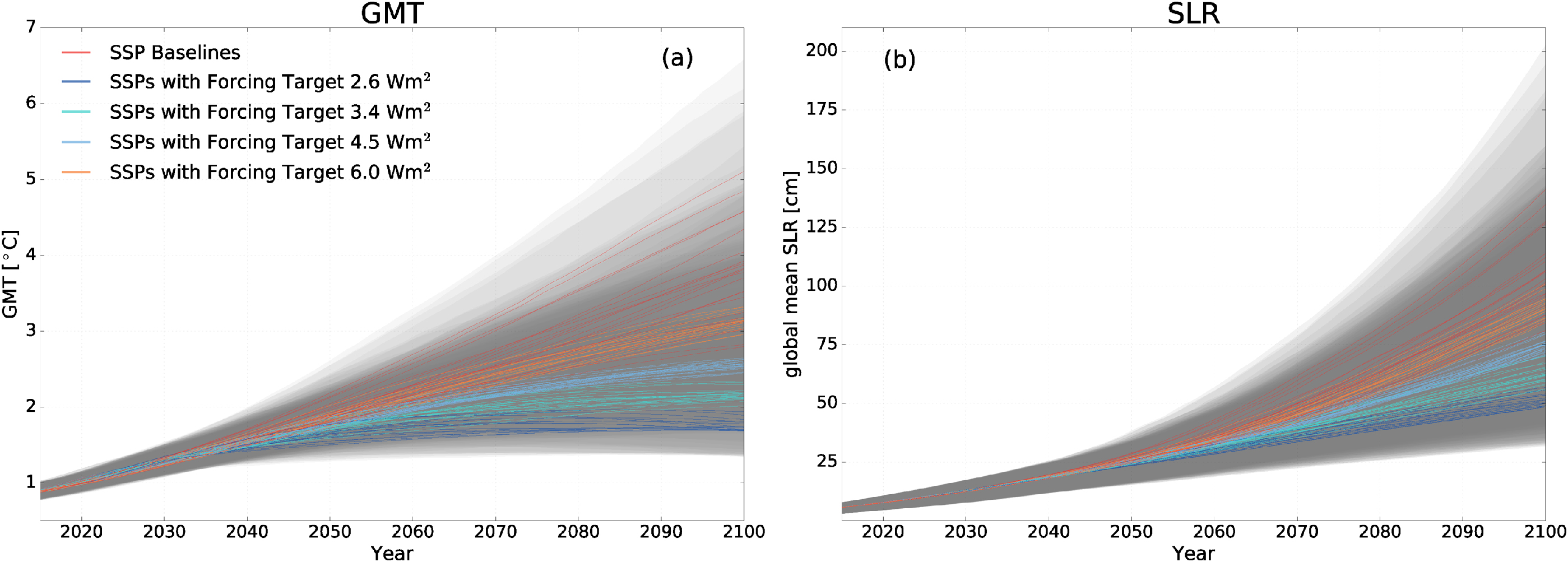
Figure 1. Probabilistic MAGICC global mean temperature (GMT) (a) and global mean sea level rise (SLR) projections (b) with medians and corresponding gray shaded 66% ranges for each member of the SSP scenario ensemble, color coded by specific 2100 radiative forcing targets. Baseline scenario medians are shown in red. GMT anomalies in °C are provided relative to 1850, global mean SLR is given in centimeters relative to the 1986–2005 mean.
Download figure:
Standard image High-resolution image
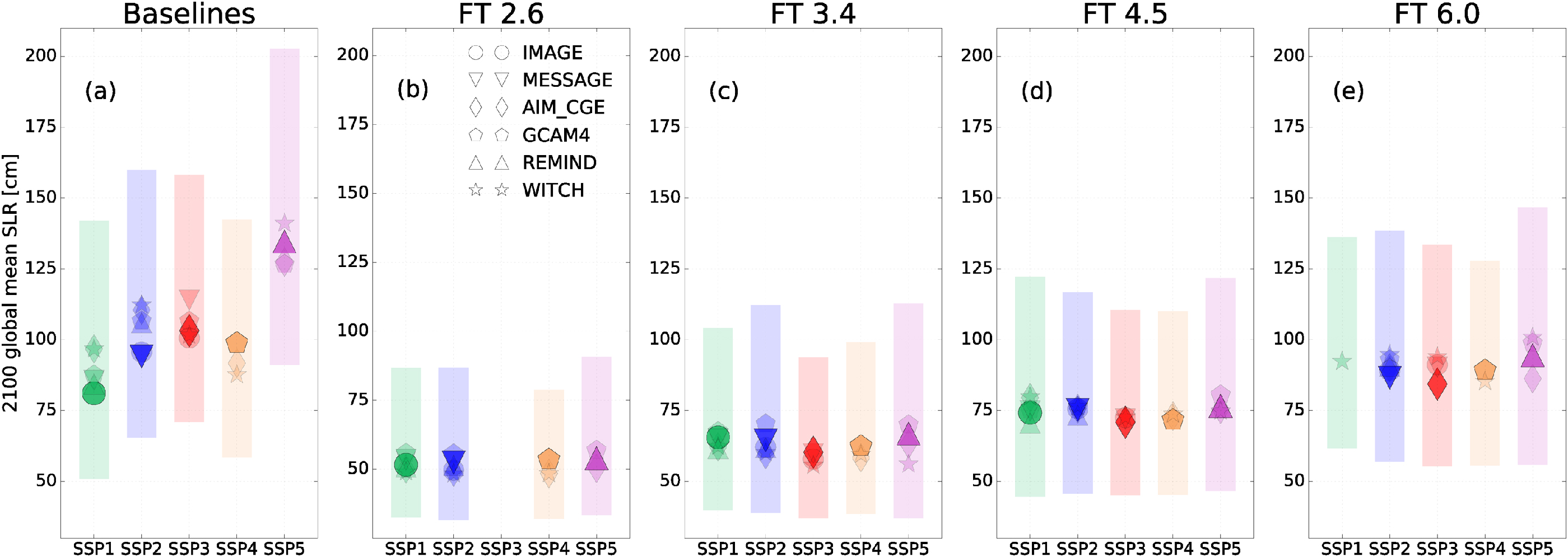
Figure 2. Probabilistic 2100 global mean SLR projections for SSP marker scenarios, showing medians and minimum/maximum 66% ranges for the individual pathways pooled by their radiative forcing targets (FTs) and the SSP baseline scenarios. Please note that there are no FT 2.6 realizations available for SSP3, and only one model reaches 6 Wm−2 of forcing in 2100 under SSP1 assumptions. Global mean SLR is provided in centimeters relative to the 1986–2005 mean.
Download figure:
Standard image High-resolution imageTable 1. Median estimates and corresponding 66% ranges for global mean SLR projections for quantified SSP scenarios towards the end of the 21st century relative to 1986–2005. The SSPs are pooled according to their radiative forcing targets (FTs) and the baseline scenarios without any climate mitigation policies. Absolute SLR estimates are provided in centimeters, the annual rates are given in millimeters per year.
| SSP SLR | FT 2.6 | FT 3.4 | FT 4.5 | FT 6.0 | Baselines |
|---|---|---|---|---|---|
| 2100 [cm rel. to 1986–2005] | 51.5 [34.1–75.3] | 61.8 [40.2–96.4] | 74.7 [46.5–113.1] | 91.4 [60.8–131.7] | 103.3 [69.7–150.8] |
| 2081–2100 [cm rel. to 1986–2005] | 46.9 [31.2–67.4] | 54.7 [35.9–82.1] | 63.6 [40.5–94.4] | 75.8 [49.5–107.8] | 84.0 [56.2–120.9] |
| 2081–2100 avg. rate [mm yr−1] | 4.7 [3.0–8.1] | 7.2 [4.3–14.0] | 10.9 [5.8–18.3] | 15.2 [10.7–23.1] | 18.5 [13.1–28.7] |
Table 2. 2081–2100 global mean SLR projections for the main sea level components in centimeters relative to 1986–2005, median estimates and corresponding 66% ranges. SMB = surface mass balance. SID = solid ice discharge. The Antarctic SID contribution is based on results from DeConto and Pollard (2016). The quantified SSP scenarios are pooled according to their radiative forcing targets (FTs) and the baseline scenarios without any climate mitigation policies.
| Sea level component | FT 2.6 | FT 3.4 | FT 4.5 | FT 6.0 | Baselines |
|---|---|---|---|---|---|
| Thermal expansion | 18.2 [11.0–25.9] | 20.6 [12.6–28.8] | 22.7 [14.1–31.3] | 25.4 [15.9–34.6] | 27.3 [17.1–37.7] |
| Glaciers | 11.5 [9.5–13.8] | 12.3 [10.2–14.5] | 12.9 [10.7–15.1] | 13.5 [11.3–15.7] | 14.0 [11.7–16.3] |
| Greenland SMB | 2.2 [1.1–3.5] | 2.5 [1.3–4.1] | 2.9 [1.6–4.6] | 3.3 [1.9–5.4] | 3.8 [2.2–6.4] |
| Greenland SID | 3.1 [2.7–3.6] | 3.2 [2.8–3.8] | 3.4 [2.9–4.1] | 3.6 [3.0–4.4] | 3.8 [3.1–4.8] |
| Antarctic SMB | −1.8 [−2.3 to −1.4] | −2.0 [−2.6 to −1.5] | −2.2 [−2.8 to −1.7] | −2.4 [−3.2 to −1.8] | −2.6 [−3.6 to −1.9] |
| Antarctic SID | 6.2 [−1.7–23.5] | 11.1 [−1.0–32.9] | 17.7 [0.5–43.2] | 25.2 [5.2–53.6] | 30.4 [9.2–62.6] |
| Land water storage | 5.7 [4.9–6.5] | 5.7 [4.9–6.5] | 5.7 [4.9–6.5] | 5.7 [4.9–6.5] | 5.7 [4.9–6.5] |
| Total | 46.9 [31.2–67.4] | 54.7 [35.9–82.1] | 63.6 [40.5–94.4] | 75.8 [49.5–107.8] | 84.0 [56.2–120.9] |
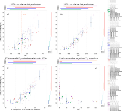
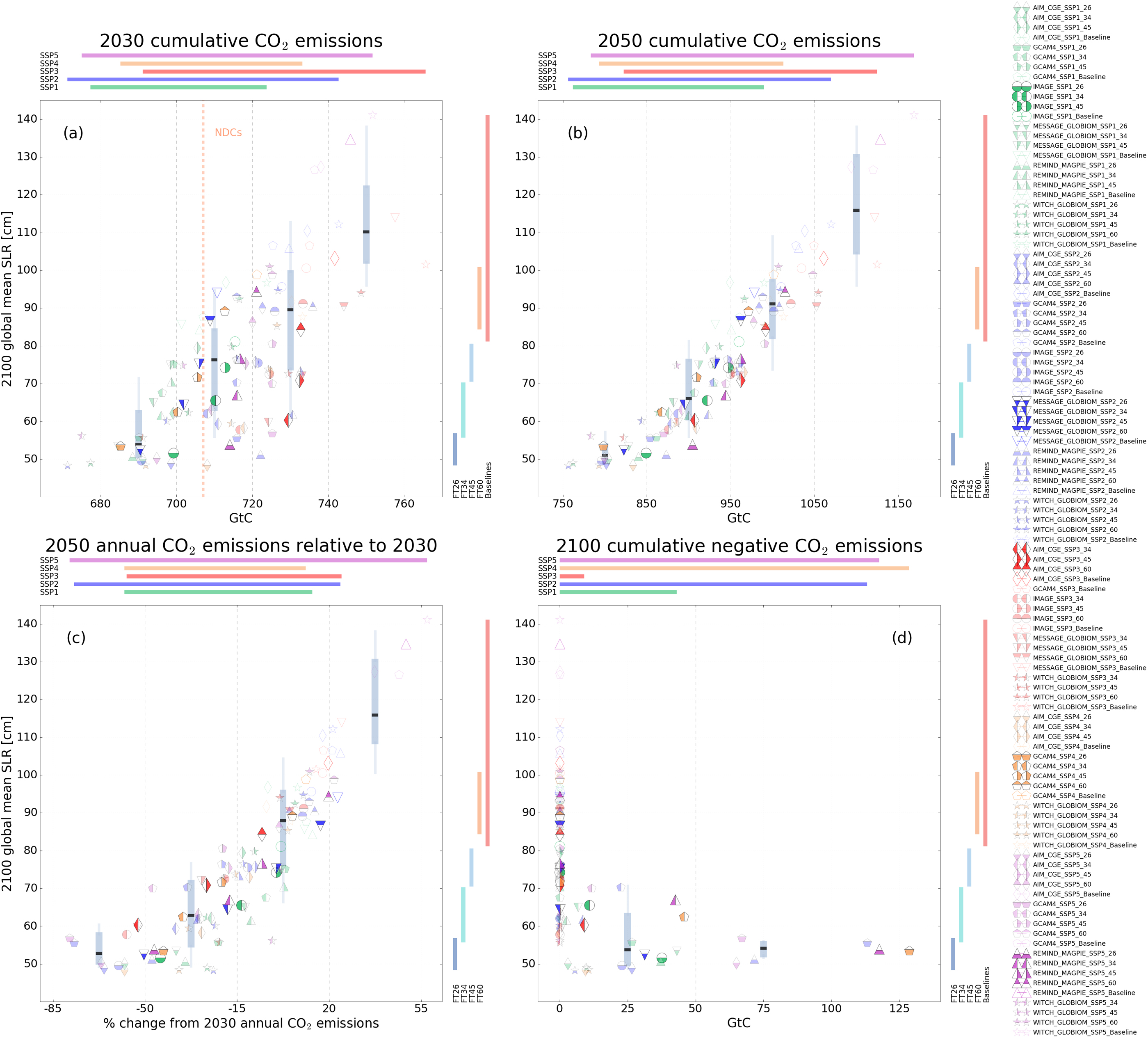
Figure 3. Emission metrics plotted against 2100 global mean SLR medians relative to 1986–2005 for every available SSP scenario. Cumulative CO2 emissions for 2030 and 2050 in GtC in panels (a) and (b), the relative change in annual CO2 emissions from 2030–2050 in panel (c) and 2100 cumulative net negative CO2 emissions in panel (d). All CO2 emissions are shown relative to pre-industrial levels. The SSP scenarios are listed with colors indicating the SSP category and symbols referencing the specific FT. The highlighted SSPs represent the marker scenarios for each SSP category. SSP and FT bars on the sides of the panels show corresponding min/max ranges. Vertical boxplots with 90% range whiskers, 50% range boxes and black medians subsume SLR trajectories falling under the individual emission metric categories. Dashed vertical gray lines indicate the category bounds in each panel. The level of cumulative CO2 emissions currently resulting from the Nationally Determined Contributions (NDCs) (UNFCCC 2016) is shown as dashed orange line in panel (a).
Download figure:
Standard image High-resolution imageResults
We show the resulting projections of global mean temperature and global mean SLR for all SSP scenarios in figure 1. SLR varies strongly between non-mitigation baseline scenarios because the varying socioeconomic assumptions for the SSPs result in different emission and temperature outcomes (figure 2(a)). Median estimates for 2100 SLR across all SSP realizations range from 89 cm (likely range: 57–130 cm) for SSP1, 105 cm (73–150 cm) for SSP2, 105 cm (75–147 cm) for SSP3, 93 cm (63–133 cm) for SSP4, 132 cm (95–189 cm) for SSP5.
Year-2100 SLR does not only depend on the end-of-century FT, but also on the pathway towards achieving this target. Nevertheless, SSP-FT SLR projections are dominated by the different FTs, with the SLR responses converging for each FT category, as opposed to the socioeconomic uncertainty driving the variation across the baseline scenarios (compare figures 2(b)–(e). 2100 median SLR is projected to be 52 cm (likely range: 34–75 cm ) for the most ambitious climate mitigation efforts framed under FT 2.6, 62 cm (40–96 cm) under FT 3.4, 75 cm (47–113 cm) under FT 4.5, and 91 cm (61–132 cm) under FT 6.0. The highest individual likely SLR estimate for a scenario under a specific SSP-FT combination is 202 cm (WITCH SSP5 baseline), the respective lowest likely projection yields around 32 cm (WITCH SSP2 FT 2.6) in 2100 (see figure 2). Average 2081–2100 SLR rates range from 5 mm yr−1 for FT 2.6 to 19 mm yr−1 for the baseline scenarios (see table 1 for more details). The 2081–2100 median SLR contributions per sea level component are listed in table 2.
With the quantitative socioeconomic information of the SSPs, SLR can be linked to specific socioeconomic metrics. We here analyze 2100 global mean SLR medians for every SSP scenario in relation to four different CO2 emission metrics, which reflect salient characteristics of the SSP emission trajectories (see figure 3): cumulative CO2 emissions since pre-industrial times until 2030 and 2050, decarbonization rates between 2030 and 2050, and cumulative net negative emissions until 2100.
Cumulative CO2 emissions until 2030 appear to relate linearly to global mean SLR in 2100, but with a large spread (figure 3(a)). The relation is more distinct for 2050 cumulative CO2 emissions (figure 3(b)). Already in 2030, limiting median SLR to below 90 cm is inconsistent with high emission pathways that have cumulative CO2 emissions above around 740 GtC. To put current mitigation pledges into perspective, we show the 2030 cumulative CO2 emissions that would result from the Nationally Determined Contributions (NDCs), which capture national post-2020 mitigation pledges under the Paris Agreement (figure 3(a), dashed orange line). Globally aggregated, they currently amount to 708 GtC since pre-industrial times until 2030 (UNFCCC 2016). Our analysis indicates that cumulative CO2 emissions until 2050 of less than 850 GtC relative to pre-industrial levels would limit 2100 median SLR to around 51 cm (90% range: 49–56 cm). In order to meet these SLR estimates, the remaining budget for the 2030–2050 period would be 142 GtC based on current NDCs. SLR increases rapidly for cumulative emission budgets exceeding this level. Figure 3(c) illustrates the relevance of rapid decarbonization between 2030 and 2050, with all pathways that show reductions of more than 50% in 2050 relative to 2030 pointing to median 2100 SLR of around 60 cm or less. If average annual CO2 emissions are still to increase over the period 2030–2050 by 20% or more relative to 2030 levels, we estimate median 2100 SLR responses of around 115 cm (100–138 cm).
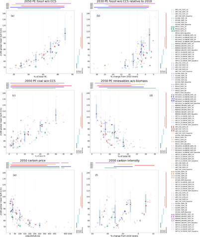
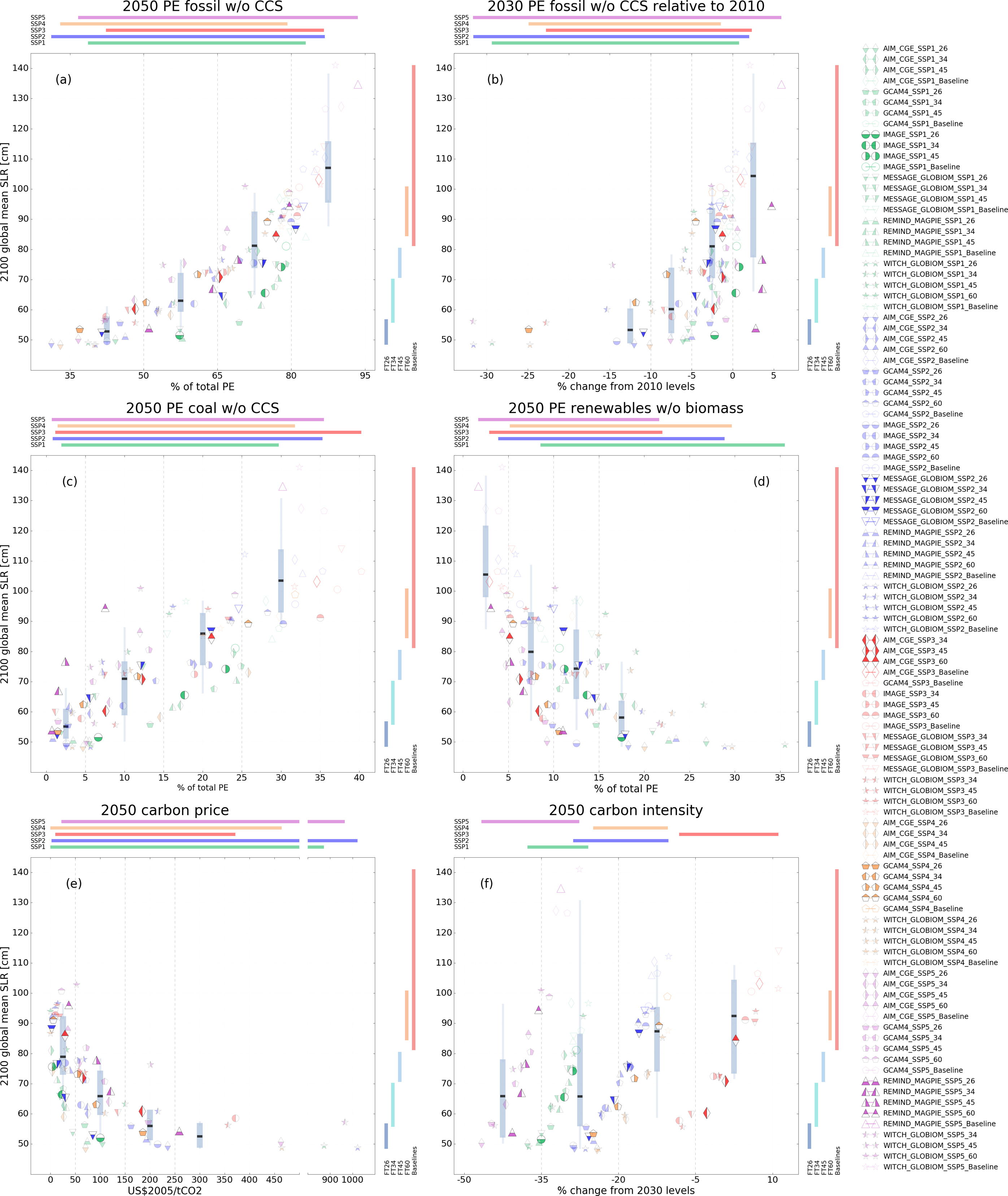
Figure 4. Selected SSP indicators plotted against 2100 global mean SLR medians relative to 1986–2005 for every available SSP scenario. The fractions of 2050 primary energy (PE) from non-CCS fossil fuels and 2050 PE from non-biomass renewable energy of 2050 total PE in panels (a) and (c), their relative changes between 2010 and 2030 as percentage from 2010 levels in panels (b) and (d); 2050 carbon price (US$2005 tCO2−1) in panel (e), percentage change of 2050 carbon intensity relative to 2030 levels in panel (f). PE is expressed using the direct energy equivalence method. The SSP scenarios are listed with colors indicating the SSP category and symbols referencing the specific FT. The highlighted pathways represent the marker scenarios for each SSP category. SSP and FT bars on the sides of the panels show corresponding min/max ranges. Vertical boxplots with 90% range whiskers, 50% range boxes and black medians subsume SLR trajectories falling under the individual SSP indicator categories. Dashed vertical gray lines indicate the category bounds in each panel.
Download figure:
Standard image High-resolution image
Figure 5. 21st century global mean SLR projections with median and shaded 66% model ranges under SSP5 baseline as well as FT 2.6 scenarios for IPCC AR5 consistent projections (dashed line) and revised SLR modeling results based on AIS contributions suggested by DeConto and Pollard (2016) (solid line). IPCC AR5 consistent SLR likely ranges for the RCPs are based on Nauels et al (2017). Global mean SLR is provided in centimeters relative to the 1986–2005 mean.
Download figure:
Standard image High-resolution image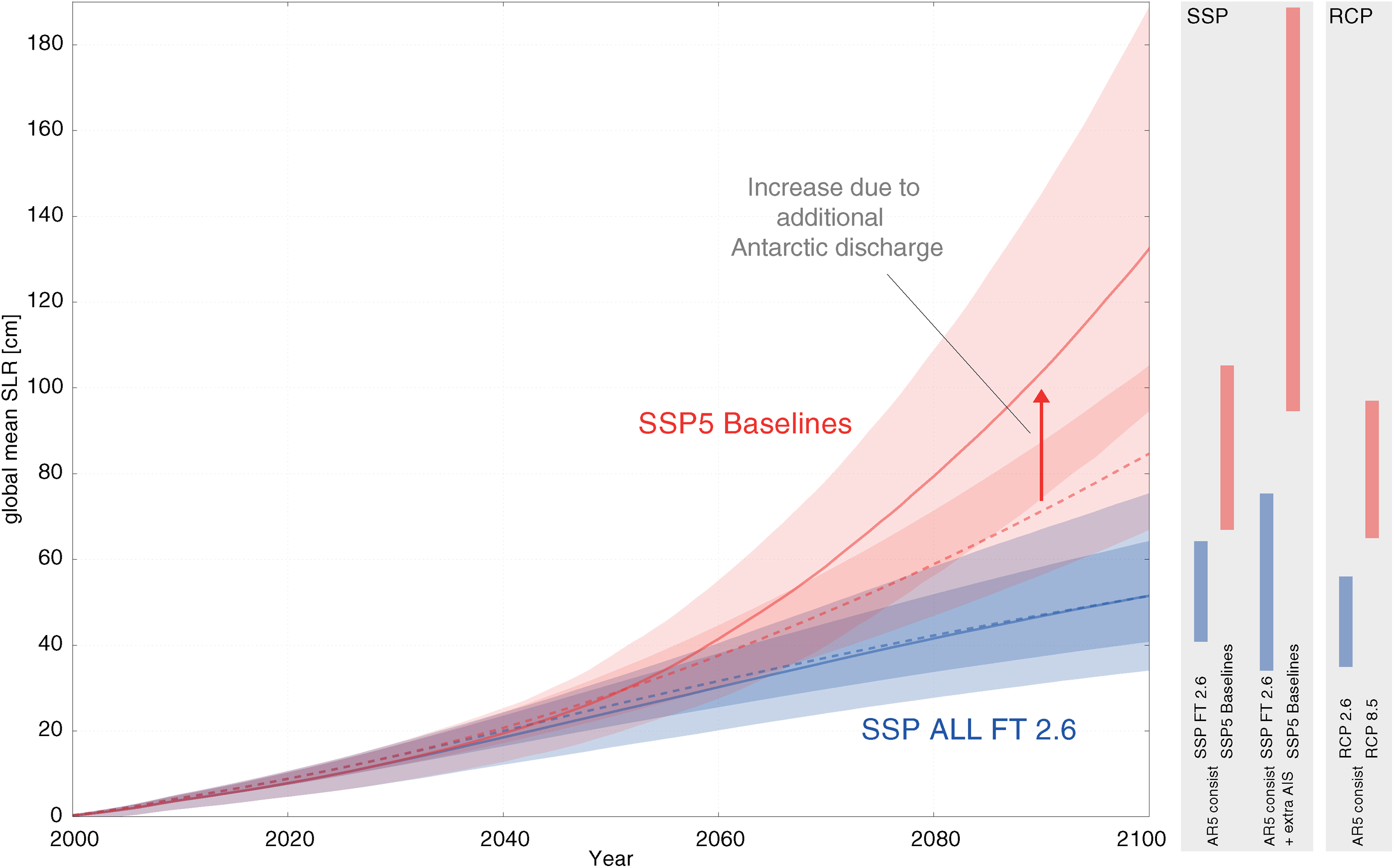
We project minimum 2100 median SLR of just above 55 cm for SSP mitigation pathways without any net negative emissions until 2100 (figure 3(d)). The SSP scenarios that show cumulative net negative emissions of up to 50 GtC throughout the second half of the 21st century show median 2100 SLR estimates of around 54 cm (49−70 cm). Under all FT 2.6 scenarios, sizable cumulative net negative emissions ranging from around 3 GtC–128 GtC are realized between 2050 and 2100, keeping the 2100 median SLR between 50 cm and 55 cm relative to 1986–2005. It is important to note that these correlations do not imply causality, but only reflect how SSP scenario characteristics project onto future SLR estimates.
Selected SSP energy and economic indicators which illustrate the transformation in the global energy system are plotted against corresponding 2100 median SLR responses in figure 4. We choose four indicators that reflect future decarbonization and early climate mitigation efforts: the fraction of primary energy (PE) from fossil fuels without carbon capture and storage (CCS) in 2050 (panel (a)), the respective relative changes between 2010 and 2030 (panel (b)), the 2050 fraction of PE from coal without CCS (panel (c)), and the 2050 fraction of PE from renewable sources without biomass (panel (d)). When PE from fossil fuels without CCS is reduced to less than 50% of total PE in 2050, the available SSP scenarios show 2100 median SLR of around 53 cm (49−61 cm). Similar median SLR estimates of 53 cm (49–63 cm) and 55 cm (49−68 cm) are linked to a 2010–2030 non-CCS fossil PE reduction rate of at least 10% and a 2050 non-CCS coal PE share of less than 5%, respectively. Under the SSP scenarios, realizing more than 15% of 2050 PE from non-biomass renewables (solar, wind, hydroelectric, geothermal energy, computed with the direct energy equivalence accounting method) would lead to 2100 median SLR estimates of around 58 cm (49−76 cm). An early reduction in the fossil-fuel share of PE correlates positively with limiting 2100 SLR (figure 4, panel (b)). Nonetheless, the overall picture for early decarbonization efforts is not fully conclusive. Fossil-fuel growth and low renewable implementation trajectories, like REMIND SSP5 FT 2.6, can still achieve 2100 median SLR of around 54 cm relative to 1986–2005 due to extreme reduction rates post 2030 (Kriegler et al 2017).
Besides the four decarbonization indicators, we also look at carbon prices and their relationship to SLR. The carbon price for achieving a specific FT varies widely (Clarke et al 2014). This high variability is also reflected in recent research on potential 1.5 °C pathways (Rogelj et al 2015), which suggests a 2050 carbon price of at least 100 US$2005 tCO2−1. Most of the SSP mitigation scenarios, however, have a 2050 carbon price of less than 100 US$2005 tCO2−1, with an unclear impact of carbon price level on 2100 SLR (figure 4, panel (e)). For the FT 2.6 pathways, 2050 carbon prices assumptions range from around 40 US$2005 tCO2−1 to more than 1000 US$2005 tCO2−1, yielding an overall minimum median 2100 SLR of around 49 cm. A 2050 carbon price of 100 US$2005 tCO2−1 would correspond to an overall 2100 median SLR of around 65 cm based on the SSP scenarios.
Finally, we also show how SLR varies with changes in the carbon intensity of GDP (figure 4, panel (f)). Every SSP follows a distinct GDP trajectory that dominates over the FT related dynamics in most scenarios. Interpretation of this metric is additionally hampered by the fact that it can easily mask increasing use of energy as long as GDP grows at a faster rate. The high reduction rates in carbon intensity for SSP5 are predominantly caused by the highest GDP growth regime of all SSPs. As such, carbon intensity fails as a predictor for 2100 SLR projections.
All analyses presented in the figures and tables are also provided for IPCC AR5 consistent global mean SLR projections in the supplementary information, available at stacks.iop.org/ERL/12/114002/mmedia. In order to highlight the difference in the SLR projections for the AR5 consistent setup and the estimates including the revised Antarctic contribution based on (DeConto and Pollard 2016), we compare both setups for the non-mitigation SSP5 baseline scenarios, which are similar to RCP8.5, and the strongest mitigation efforts represented by FT 2.6 in figure 5. 2100 median SLR estimates for the SSP5 baseline scenarios are almost 50 cm higher for the projections including the additional Antarctic rapid dynamics compared to the IPCC AR5 consistent projections. The SSP FT 2.6 estimates practically do not change except for a wider 66% model range when the additional rapid dynamics are included. We have also included the 2100 RCP 2.6 and RCP 8.5 likely ranges for the IPCC AR5 consistent setup (Nauels et al 2017), showing overall slightly lower SLR likely ranges for RCP 2.6 compared to SSP FT 2.6 and for RCP 8.5 compared to the SSP5 baseline scenario.
Discussion
Compared to the previous RCP scenario generation, the SSP-FT framework allows to more directly relate future physical responses of the climate system to the underlying socioeconomic assumptions of the scenario trajectories. We apply a process-based probabilistic sea level emulator in conjunction with the widely-used simple climate carbon-cycle model MAGICC to provide a preview of global mean SLR projections associated with the full set of SSP scenarios.
The revised sea level estimates from Antarctica based on results from DeConto and Pollard (2016) alter total global mean SLR projections dramatically for high emission pathways (see figure 5). The extremely high SLR estimates for the non-mitigation baseline scenarios, in particular the SSP5 projections with highest individual 2100 likely ranges of around 200 cm (see figure 2(a)), highlight that ambitious climate policies are needed to avoid the most severe impacts from rising sea levels around the globe. As such, these higher estimates point to a growing risk of potentially catastrophic sea level rise by the end of the 21st century under unchecked climate change. However, the revised estimates also indicate that strong mitigation efforts could prevent the onset of the rapid dynamics that cause the additional sea level contribution from the Antarctic ice sheets (see figure 5).
The SSP5 baseline emission pathway is very similar to RCP8.5 (Kriegler et al 2017), which allows us to relate our corresponding SLR projections directly to other studies that provide 2100 RCP8.5 projections and account for the additional AIS discharge processes suggested by DeConto and Pollard (2016). Our 2100 median SSP5 baseline estimate of around 132 cm is lower than the suggested 150–184 cm 2100 RCP8.5 median range by Bars et al (2017) who use statistical methods to account for the additional AIS rapid discharge. Our median estimates are also below the corresponding 150 cm by Wong et al (2017a).
Our calibration results suggest threshold temperatures between 0 °C and 3.2 °C above 1850 levels for triggering an additional annual discharge rate, with 25 of the 29 calibrated parameter sets showing threshold temperatures between around 1.9 °C and 3.2 °C (see table S1). The latter values are similar to the threshold values of 1.9 °C−3.1 °C derived by Wong et al (2017a) for a similar parameterization. These estimates make a strong case for limiting warming in accordance with the climate targets of the Paris Agreement (holding warming well below 2.0 °C and pursuing to limit it to 1.5 °C above pre-industrial levels). Our global AIS SID parameterization does not incorporate regional ice sheet characteristics like e.g. Ritz et al (2015) (see the supplementary information for more details). Therefore, the presented temperature thresholds have to be interpreted and discussed in light of these limitations.
In order to inform the mitigation requirements to limit long-term SLR under the SSPs, we have selected several CO2 emission, energy and economic indicators to explore the specific SSP assumptions that result in the respective FT trajectories. The applied suite of metrics assists with translating the necessary efforts to limit global mean SLR projections into the actual processes that transform the energy system with some of its associated costs, like the carbon price. Even the highest carbon price or strongest available SSP climate mitigation pathway does not stabilize SLR by 2100 in our simulations. The long memory of the SLR components will cause continued SLR well beyond the 21st century. To allow for a more in-depth investigation of minimizing long-term SLR under the SSPs, trajectories consistent with a 1.5 °C climate target and more sophisticated post-2100 extensions are needed.
The SSP-FT analysis, as presented here, allows for a first linkage of mitigation efforts, SLR impacts and adaptation costs. Impact-relevant socioeconomic indicators, like future GDP and population growth as well as urbanization dynamics, differ widely between the different SSPs and so do the projected SLR impacts. Global analysis of SLR impacts under different FT and SSP scenarios has shown that key impact metrics, like affected people and coastal flood costs, depend equally as much on the SSPs as on different FTs (Hinkel et al 2014). It is worth noting, however, that these estimates are based on lower levels of 21st century global mean SLR than those presented here. Furthermore, research on global mean SLR has to be merged with projections on regional extreme sea level exposure to allow for a comprehensive assessment of SLR impacts (Muis et al 2017). Corresponding estimates critically depend on assumptions about future coastal adaptation, which in return also depend on regional development trajectories. Given the anticipated socioeconomic development in coastal regions, adaptation will need to reduce future physical flood probabilities below present values to maintain present flood risk (Hallegatte et al 2013).
To link global socioeconomic requirements under different SSP-FTs to coastal impacts, regional downscaling of the global mean SLR trajectories presented here is required as well as merging them with local coastal impact models (Hinkel and Klein 2009). This would allow for an integrated comparison of mitigation requirements with impact metrics that can inform decision making and risk assessments on a regional level.
Acknowledgments
We acknowledge the International Institute for Applied Systems Analysis (IIASA) which is hosting the SSP scenario database (https://tntcat.iiasa.ac.at/SspDb/). We would also like to thank R DeConto for providing the calibration data used in this study. M Meinshausen receives the Australian Research Council (ARC) Future Fellowship Grant FT130100809. M Mengel is supported by the AXA Research Fund. C-F Schleussner acknowledges support by the German Federal Ministry for the Environment, Nature Conservation and Nuclear Safety (16_II_148_Global_A_IMPACT). J Rogelj acknowledges support of the Oxford Martin School Visiting Fellowship Programme.
ORCID iDS
Alexander Nauels https://orcid.org/0000-0003-1378-3377
Joeri Rogelj https://orcid.org/0000-0003-2056-9061
Malte Meinshausen https://orcid.org/0000-0003-4048-3521
Carl-Friedrich Schleussner https://orcid.org/0000-0001-8471-848X)
Matthias Mengel https://orcid.org/0000-0001-6724-9685).