

Abstract
How the pattern of the Earth's surface warming will change under global warming represents a fundamental question for our understanding of the climate system with implications for regional projections. Despite the importance of this problem there have been few analyses of nonlinear local temperature change as a function of global warming. Individual climate models project nonlinearities, but drivers of nonlinear local change are poorly understood. Here, I present a framework for the identification and quantification of local nonlinearities using a time-slice analysis of a multi-model ensemble. Accelerated local warming is more likely over land than ocean per unit global warming. By examining changes across the model ensemble, I show that models that exhibit summertime drying over mid-latitude land regions, such as in central Europe, tend to also project locally accelerated warming relative to global warming, and vice versa. A case study illustrating some uses of this framework for nonlinearity identification and analysis is presented for north-eastern Australia. In this region, model nonlinear warming in summertime is strongly connected to changes in precipitation, incoming shortwave radiation, and evaporative fraction. In north-eastern Australia, model nonlinearity is also connected to projections for El Niño. Uncertainty in nonlinear local warming patterns contributes to the spread in regional climate projections, so attempts to constrain projections are explored. This study provides a framework for the identification of local temperature nonlinearities as a function of global warming and analysis of associated drivers under prescribed global warming levels.
Export citation and abstract BibTeX RIS

Original content from this work may be used under the terms of the Creative Commons Attribution 3.0 licence. Any further distribution of this work must maintain attribution to the author(s) and the title of the work, journal citation and DOI.
1. Introduction
As the world warms there are observed patterns of local warming, such as arctic amplification and increased warming over land than ocean (Braganza et al 2003, Drost and Karoly 2012). However, the pattern of warming may change in a warmer world, with some locations experiencing an accelerated or decelerated warming per unit change in global warming as illustrated using idealised examples in figure 1(a). Nonlinear local change could occur due to factors such as changes in non-greenhouse gas forcings (Good et al 2015, King et al 2018), movement in storm tracks (Arblaster and Meehl 2006, Knutti et al 2015) or shifting sea-ice boundaries. Previous studies have analysed the validity of assuming the pattern of warming will not change (through methods often referred to as 'pattern scaling' first proposed by Santer et al (1990)) and found that for single- or multi-model ensemble average changes the assumption of linearity largely holds (Frieler et al 2012, Tebaldi and Arblaster 2014, Seneviratne et al 2016, King et al 2018, Osborn et al 2018, Tebaldi and Knutti 2018). The efficacy of pattern scaling has been discussed in reports from the Intergovernmental Panel on Climate Change (e.g. IPCC fifth assessment report; Collins et al 2013) with the view that in general, under transient global warming, the use of pattern scaling for large-scale projections holds. However, individual models within an ensemble have considerable departures from linear warming that cannot be ruled out (King et al 2018). The factors determining why different models may produce varying degrees of nonlinear change have not been explored previously.
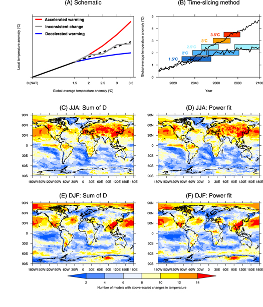
Figure 1. Schematics illustrating nonlinearity identification for local temperatures and time-sampling method for two projections of global mean temperature, and maps showing model agreement using different schemes for nonlinear change identification. (a) A schematic showing how consistent nonlinearities in local temperatures are identified for idealised examples where there is consistent nonlinear warming (red), consistent nonlinear cooling (blue) and inconsistent change (grey). (b) A schematic showing the time-samples taken from ACCESS1.3 RCP8.5 and RCP4.5 simulations to represent the model world at each global temperature increment. (c)–(f) Model agreement in sign of nonlinearity in (c), (d) boreal summer and (e), (f) in boreal winter, using the (c), (e) summed departures from linearity and (d), (f) power fit methodologies.
Download figure:
Standard image High-resolution imageIt is vital that we have a fuller understanding of whether local temperatures will scale linearly with global warming; an incorrect assumption of linearity in regional climate projections would result in a lack of preparedness for new local climates and associated extremes. If there are projected nonlinear warming patterns, it is important the processes causing these local accelerations or decelerations are well understood. A comprehensive analysis of the identification and processes behind nonlinear local temperature change using models in the fifth phase of the Coupled Model Intercomparison Project (CMIP5; Taylor et al 2012) has not been undertaken previously. Given these models are often used for climate projections (e.g. Collins et al 2013), or to drive regional climate models for local projections (e.g. Evans et al 2014), an analysis of nonlinear change in these models would be of great use.
The consequences of nonlinear local temperature change for associated changes in extremes are also under-explored. A cursory analysis of East Asian extreme high summer temperatures with and without pattern scaling at 2 °C global warming indicated assumption of a linear local response to global warming would result in divergent projections from those directly simulated by CMIP5 models (King et al 2018). Given that local temperature nonlinearities may be associated with changes in other atmospheric variables (King et al 2018) and that extreme events, such as heatwaves, are often associated with the confluence of multiple processes (Hauser et al 2016, Donat et al 2017) then one might expect that nonlinear temperature change and changes in associated processes, that likely differ between models, would strongly influence extremes projections.
In this study, methodologies for the estimation of nonlinear change were explored and a framework for quantifying nonlinear change was developed. Using a multi-model ensemble, the associations between nonlinear local temperature change and changes in other atmospheric variables were explored. Finally, a case study regional analysis of nonlinear change was conducted to illustrate the uses of the methodology proposed here for examining processes behind nonlinearity and consequences for extremes.
2. Data and methods
Here, I propose a method for analysing nonlinear temperature changes using time-slices of projections (figure 1(b); Schleussner et al 2016, James et al 2017, King et al 2017), under different greenhouse gas emissions scenarios, from 16 CMIP5 climate models. Surface air temperature data ('tas') from the CMIP5 models were used to generate estimates of a pre-industrial climate (the average global annual surface temperature in historicalNat simulations for 1901–2005) and the timeslices of 1.5 °C, 2 °C, 2.5 °C, 3 °C and 3.5 °C warmer worlds (all years within decades where the global-average decadal-average temperature is within 0.2 °C of the desired global warming level from RCP2.6, RCP4.5, RCP6.0 and RCP8.5 simulations for 2006–2100) following the method described in King et al (2017). This process was designed to generate ensembles which include model years that adequately sample the range of internal climate variability, for example, a proportionate set of El Niño and La Niña events, within each global warming level. This timeslice method was also used to examine local temperature nonlinearities at the Paris Agreement global warming limits previously (King et al 2018). The use of a timeslice method removes uncertainties associated with scenario choice and different model climate sensitivity values (Hawkins and Sutton 2009) allowing for analysis across models for a given level of global warming. All the models and experiments used in this analysis are listed in supplementary table S1, which is available online at stacks.iop.org/ERL/14/064005/mmedia. All model data were interpolated onto a common regular 2° grid.
2.1. Methods for estimating nonlinearity in local temperatures: the sum of departures
The nonlinearity in temperatures was calculated using two methods referred to here as (1) the sum of departures from linearity and (2) the power fit. The sum of departures from linearity is an extension of the methodology employed by King et al (2018). The linearity of the local temperature change was assessed by comparing the model-simulated local temperature at a given level of global warming with the linear extension of local warming from 0.5 °C less global warming. The local departure from linearity, D, for each level of global warming is defined as:
where TSimulated to x°C is the local median model-simulated temperature at a given level, x, of global warming. The multiple from the lower level of global warming (x/x − 0.5) was used to apply the local linear extension from the previous level of global warming above pre-industrial conditions in the model simulations. These departures from linearity were calculated for global warming worlds of 2 °C, 2.5 °C, 3 °C and 3.5 °C above pre-industrial levels. Dx was calculated in individual models and the model ensemble-median for seasonal-average temperatures. The sum of Dx, ΣDx, across the four global warming levels, was also computed at each gridbox in each individual model and in the multi-model ensemble median. The scaling departures were computed based on long reference periods with 0.5 °C extensions, so as to better estimate the forced response and reduce the effect of internal variability in the results (King et al 2018). The comparison between the scaled and simulated average local temperatures for a given level of global warming makes use of the forced response to the given global warming level and means that scaling downwards from a higher level of warming (Tebaldi and Knutti 2018) produces very similar results. King et al (2018) describes many sensitivity tests that were performed to ensure the robustness of this general method that is here applied to higher global warming levels. Further sensitivity tests were performed for this analysis and are described in the supplementary material.
The multi-model ensemble median signal-to-noise of nonlinearity was calculated to provide an indication of the magnitude and confidence in nonlinear temperature changes. The signal was simply defined as the multi-model ensemble median value of ΣDx while the noise was estimated as the standard deviation across the 16 individual climate models. This is the same definition as used by King et al (2018), but with a combination of values of Dx across the four global warming levels.
2.2. Methods for estimating nonlinearity in local temperatures: the power fit
The second method involves fitting a curve to the local temperatures as a function of global temperature and using the power to determine the nonlinearity in the local temperature response to global warming. The power fit takes the form:

where values of b are used to estimate the nonlinearity with b > 1 indicating an acceleration (similar to the red curve in figure 1(a)), and b < 1 indicating a deceleration in local warming (similar to the blue curve in figure 1(a)). The value of b was estimated after taking the natural logarithm such that the gradient of the linear fit is b.
The value of b was estimated using average local temperature values at each global warming level (1.5 °C, 2 °C, 2.5 °C, 3 °C and 3.5 °C above pre-industrial levels) for each of the 16 CMIP5 models. The level of agreement between models in whether b is greater than or less than one and the multi-model ensemble values of b at each gridbox were estimated.
Estimates of the nonlinearity in local temperatures produced using these two different methods were compared for multi-model ensemble median values and for model consistency in the sign of nonlinearity. All subsequent analysis is based only on the sum of departures method for quantifying nonlinear change.
2.3. Methodology for understanding nonlinear changes
Other data from the CMIP models and experiments were extracted for investigating changes associated with local nonlinearities in temperature change and possible causes of these nonlinearities. Model precipitation ('pr'), mean sea level pressure ('psl'), downwelling shortwave radiation at the surface ('rsds'), surface upward sensible heat flux ('hfss'), and surface upward latent heat flux ('hfls') data were extracted for each of the 16 models and experiments (table S1). The sensible and latent heat fluxes were used to derive the evaporative fraction which is defined simply as the latent heat flux divided by the sum of the latent and sensible heat fluxes. For all these variables, the local average seasonal change was computed between the 1.5 °C and 3.5 °C global warming levels.
The processes associated with nonlinearity in local temperatures were first investigated by calculating the Spearman rank correlation coefficient between the local nonlinearity in temperatures, i.e. the sum of Dx across the four global warming levels in each model, with the change in precipitation from 1.5 °C to 3.5 °C of global warming. This was computed for each season at each 2° gridbox. As there are 16 climate models that these correlations are calculated from, the required correlation coefficient for significance at the 5% level is  (under the assumption of model independence). An additional criterion aimed at minimizing the false discovery rate was also included based on ranked p-values of gridbox-based correlations (Wilks 2011, 2016) using the global test level, αglobal, of 0.1. Locations where the false discovery rate criterion is met are highlighted. Note that there is a great deal of debate around the use of statistical significance testing in atmospheric science (Nicholls 2001, Ambaum 2010). As a result, there is less focus placed here on individual correlations at gridbox level, but rather more emphasis on overall patterns and plausible mechanisms behind the statistical relationships. The statistical distributions of correlation coefficients over land and ocean areas were computed by area-weighting and aggregation of the gridbox correlations.
2.4. Case study analyses for a specific region: north-eastern Australia
To demonstrate the utility of this methodology for examining local climate changes, three regions for which the inverse relationship between model change in precipitation (ΔP) and nonlinear temperature response (ΣDx) is particularly strong were identified and further investigated. Land areas only in Western North America (120°W–105°W, 30°N–50°N), Eastern Europe (10°E–40°E, 40°N–60°N), and north-eastern Australia (135°E–155°E, 30°S–15°S) were investigated during their summer seasons (i.e. JJA for W North America and E Europe, DJF for NE Australia). The analysis in the main article focusses on north-eastern Australia only with analysis of the other two regions in supplementary material.
To investigate meteorological changes that may be associated with nonlinearity in temperatures, the model-average changes in precipitation (ΔP), mean sea level pressure (ΔMSLP), downwelling shortwave radiation at the surface (ΔRSDS), and evaporative fraction (ΔEF) were correlated at each gridbox with the model-average land-only area-average nonlinearity in temperature for each region (ΣDx) for north-eastern Australia, W North America and E Europe. Investigation of this range of dynamical and thermodynamical variables with analysis of locations beyond the specific areas of interest reveals the major differences in models associated with different nonlinear warming patterns.
The implications of model spread in nonlinear warming were investigated through examining climate projections for north-eastern Australia. The model-average area-average ΔP was plotted against the model-average area-average ΣDx. The implications of the strong inverse relationship identified between ΔP and ΣDx were examined through compositing the eight models where ΔP is greater than the model-ensemble median ΔP and the eight models where ΔP is less than the model-ensemble median ΔP and comparing projected changes in the 50th, 90th and 95th percentile summer-average temperatures. This allowed for analysis of whether the effect of different ΔP projections extends to nonlinear warming in extreme summer-average temperatures. Likelihood of exceedance of the observed record anomaly, derived from the Australian Water Availability Project (AWAP (Jones et al 2009)) gridded observational product, was computed for the two sub-ensembles at each level of global warming. The best estimate of exceedance probability was defined using the entire model sub-ensembles while the sampling uncertainty was estimated by bootstrap resampling 50% of the sub-ensemble models 10 000 times. The 90% confidence interval on the likelihood of exceedance in a given year was extracted from the ranked bootstrap values.
The north-eastern Australia region has high uncertainty in climate projections especially for model simulation of precipitation change and nonlinear temperature change. To ascertain whether the uncertainties may be constrained, two model evaluation tests were used for subsetting models to generate projections. Firstly, the observed inverse DJF P–T relationship (Nicholls 2004, King et al 2014a) over the period 1950–2005 (derived from AWAP (Jones et al 2009)) was compared with the model simulated P–T relationships in the historical runs over the same period. The eight models with inverse correlations (as measured by Spearman's rank correlation coefficients) of most similar magnitude to the observed inverse P–T relationship were selected as the best-performing models on this metric. The use of other periods of differing lengths and the regression coefficient instead of the correlation coefficient produced similar results.
This process was also repeated for sub-ensembles composed of the best-performing models in simulating the CP El Niño (Xu et al 2017). Only the seven models were selected here that also appear in table 1 of Xu et al (2017) (table S2).
As with the wet and dry model subsets, median and extreme temperature projections were analysed in these two sub-ensembles. The likelihood of exceeding the observed record at each level of global warming in each sub-ensemble was computed with the bootstrap resampling again used to estimate the 90% confidence interval.
3. Results
3.1. Global analysis
Firstly, a comparison of the two methods (the sum of departures from linearity and the power fit) to quantify nonlinearities in local temperature change was conducted. Figures 1(c)–(f) shows the level of model agreement in the sign of nonlinearity under global warming in boreal summer and winter for each method. There is a distinct seasonal cycle with model agreement towards locally accelerated warming in the northern hemisphere mid-latitudes in boreal summer, but not in winter. In addition, more models show locally accelerated warming in land regions than is simulated over the oceans. Remarkably, despite the very different statistical approaches in estimating local nonlinearities, there is strong similarity in the levels of model agreement on the sign of nonlinearity between the two methods. The pattern correlation between the levels of model agreement based on the two methods is 0.93 in both JJA and DJF. The similarity between the results of these two methods, both in model agreement and multi-model ensemble median nonlinearity (figure S5) suggests that these signals are robust and the choice of method for estimating nonlinear change does not have a large bearing on the results. All subsequent analysis is based on the sum of departures measure for nonlinearity only.
To understand the controls on nonlinear warming in the models it is useful to make comparisons between models within the CMIP5 ensemble and examine relationships with other variables (figures 2(a), (b)). Over continental land regions in summer there is a pattern of negative correlation between models, in nonlinear local temperature change (derived from the sum of departures method, ΣDx) and local change in precipitation from 1.5 °C to 3.5 °C global warming, ΔP, i.e. models which project more drying tend to project an acceleration in warming. The inverse relationship between precipitation and increased heat has been noted before, in Europe in boreal summer for example (Fischer et al 2007), but not in the context of nonlinear climate change. In western North America, central and eastern Europe, and north-eastern Australia, there are locally significant inverse relationships between ΣDx and ΔP in summer. In some locations within these three regions, the p-values associated with these correlations are small enough to also satisfy the relatively strict false discovery rate criterion. In winter, the relationship between nonlinearity in temperature and change in precipitation weakens over land and in some places, such as northern Europe, more precipitation is correlated with accelerated local warming. Over the ocean, there are more areas where the inter-model correlation between ΣDx and ΔP is positive, i.e. models with increasing precipitation in a location tend to exhibit accelerated warming at that same place. Due to the larger land area in the northern hemisphere, there is a higher proportion of overall land area where there is an inverse relationship between ΣDx and ΔP in boreal summer than in winter (figures 2(c), (d)).

Figure 2. Inter-model correlation maps of nonlinearity in local temperature and change in precipitation from 1.5 °C to 3.5 °C of global warming and histograms of their aggregates over land and ocean regions. (a) Boreal summer and (b) winter maps showing correlation coefficients between the nonlinearity in local temperature and the change in local precipitation from 1.5 °C to 3.5 °C global warming. Black stippling indicates significance at the 5% level with red circles indicating where the additional false discovery rate criterion (αFDR = 0.1) is also achieved. (c) Boreal summer and (d) winter histograms showing the percentage area of land (red) and ocean (blue) at each correlation coefficient. The dashed line marks zero and the dotted lines show where correlations become significant at the 5% level. The percentage area of land (red) and ocean (blue) for which these correlation coefficients are significant at the 5% level is shown.
Download figure:
Standard image High-resolution imageOver the oceans, accelerated local warming is associated with an increase in precipitation, in the absence of any substantial dynamically-forced change, due to the Clausius–Clapeyron relation. In a global sense, warming of the atmosphere increases precipitation at a sub-Clausius–Clapeyron rate (Allen and Ingram 2002, Held and Soden 2006). While it is of debate whether it is reasonable to connect the relationship between local temperature and precipitation change to global warming (e.g. Schroeer and Kirchengast 2018) the results here show that in most locations, or indeed an average location on the globe, the models with accelerated warming in local temperatures tend to have associated increasing local precipitation relative to other models. Using a methodological framework, such as this, where global temperature is constrained but local differences between models exist due to nonlinearities affords the potential for extending our understanding of the thermodynamic response of the hydrological cycle to climate change.
In contrast, over moisture-limited regions, such as mid-latitude land areas in summer, models with stronger precipitation reductions tend to be associated with accelerated local warming. A part of this effect could be due to circulation changes, although equivalent correlations between ΣDx and ΔMSLP (figure S6) show a very different relationship and no obvious similarity in the pattern of ΣDx–ΔP correlation. The concentrated pattern of inverse relationships over land and in summertime is suggestive of a land-surface feedback effect dominating over a circulation influence. There has been a body of research, especially focussed on European summer temperature extremes and land surface feedbacks, that suggests summer temperatures are amplified by preceding and concurrent soil moisture deficits (Seneviratne et al 2006, Fischer et al 2007, Vautard et al 2007, Lorenz et al 2010, Miralles et al 2014) and that this effect is due to drying soils resulting in reduced convection and increased sunshine intensity (e.g. Zampieri et al 2009). In central and eastern Europe, the relationship between ΣDx and ΔEF at each gridbox (figure S6) has a similarity with that of the ΣDx–ΔP relationship and indicates that in summertime, local accelerated warming occurs in models with a reduction in evaporative fraction (i.e. a reduction in latent heat flux relative to combined sensible and latent heat flux). Previous work has also suggested that as global temperature rises, the summertime climate of areas such as central and eastern Europe could become more semi-arid (Beck et al 2018) and therefore be subject to greater land-atmosphere coupling (e.g. Koster et al 2004, Seneviratne et al 2006). This analysis suggests that this shift towards a drier climate in central and eastern Europe results in an acceleration of average regional temperature rise relative to the rate of global temperature increase.
As previous analyses indicate that dry winter and spring conditions in Europe result in hotter summers or more intense summer heat extremes (Fischer et al 2007, Vautard et al 2007), a corollary in this context was investigated by plotting the local ΣDx–ΔP relationship for springtime precipitation and nonlinearity in summertime temperatures between models (figure S7). In this instance a strong relationship was not found for Europe and most other locations.
3.2. Case study regional analysis for north-eastern Australia
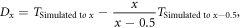
To examine the relationship between ΣDx and ΔP in more detail, north-eastern Australia, a region where the inverse relationship between ΣDx and ΔP is particularly strong and climate projections are highly uncertain (e.g. Collins et al 2013), was selected for further analysis. To explore the local meteorological drivers of nonlinear temperature change, associated changes in several relevant variables were examined (figure 3). The area-average nonlinearity in north-eastern Australia is strongly correlated with the level of local warming in the central Pacific (CP; figure 3(a)). Over north-eastern Australia, model accelerated warming is strongly connected to locally reduced precipitation (figure 3(b)), increased incoming shortwave radiation at the surface (figure 3(d)) and reduced evaporative fraction (figure 3(e)). There are also associations with the CP whereby model accelerated warming in north-eastern Australia summer temperatures is associated with increased rainfall, decreased mean sea level pressure and decreased incoming shortwave radiation at the surface over the CP. The correlations suggest models with a tendency towards more CP El Niño conditions in future, project accelerated warming in north-eastern Australia. Over other moisture-limited regions, including western North America and eastern Europe, accelerated local warming also tends to occur in models with locally reduced evaporative fraction and increased sunshine intensity (figure S8).
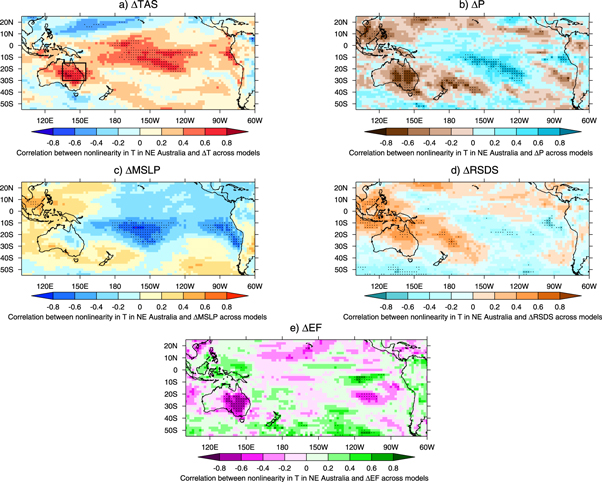
Figure 3. Regional modelled nonlinear temperature changes are strongly associated with changes to precipitation and other variables. Inter-model correlation coefficients between area-average summertime temperature nonlinearities in north-eastern Australia and the change in summertime (a) temperature, (b) precipitation, (c) mean sea level pressure, (d) downwelling shortwave radiation at the surface, and (e) evaporative fraction, respectively. Stippling indicates correlation coefficients are significant at the 5% level with red circles indicating where the additional false discovery rate criterion (αFDR = 0.1) is also achieved. Summertime is December–February in north-eastern Australia.
Download figure:
Standard image High-resolution imageThe implications of nonlinearities for model projections were explored further for north-eastern Australia. The ranges of projections for nonlinear temperature change and precipitation change in north-eastern Australia are large (figure 4(a)) and interconnected. This results in alternative projections for north-eastern Australia of drier and much hotter summers or wetter and warmer summers. Grouping model projections of only the wetter 50% of models and drier 50% of models illustrates this divergence in both the mean and hot extremes between these sub-ensembles (figure 4(d)). The dry models have 0.6 °C additional warming in the median above that simulated in the wet sub-ensemble between 1.5 °C and 3.5 °C global warming. There is also additional warming in the 90th and 95th percentile summer temperatures in the dry sub-ensemble of 0.41 °C and 0.51 °C respectively. Furthermore, the impact of these divergent projections can be seen through the differing probabilities of exceeding the observed record hot summer in each sub-ensemble (figure 4(g)). The effect of uncertain precipitation projections on the chance of summer temperatures exceeding the observed record is roughly equivalent to the effect of 0.5 °C of global warming.
Figure 4. The effect of nonlinear temperature projections on average and extreme summer temperatures. (a) Scatter between area-average change in precipitation and nonlinearity in temperature for NE Australia. Models with a wetting (drying) tendency relative to the multi-model median are marked in blue (brown). The correlation coefficient is shown. (b), (c) As (a) but with best-performing models for interannual P–T relationship and CP ENSO representation highlighted (black crosses) respectively. (d) The multi-model ensemble median (solid), 90th percentile (dashed) and 95th percentile (dotted) area-average summer temperatures at each increment of global warming are shown for the wetter 50% of models (blue) and the drier 50% of models (brown) for NE Australia. (e), (f) As (d) but with best-performing sub-ensembles for P–T relationship and CP ENSO relationship shown in black. (g) Projected probability of exceedance of the observed record hot summer in NE Australia in a given year under each global warming level in wetter (drier) 50% of models in blue (brown). Best estimates are shown as bars with 90% confidence intervals as black lines. (h), (i) As (g) but also for the best-performing sub-ensembles for P–T relationship and CP ENSO relationship shown in grey bars.
Download figure:
Standard image High-resolution image
Methods for constraining projections where model nonlinearities are associated with high uncertainty were explored. In moisture-limited regions, including continental Europe (Fischer et al 2007, Vogel et al 2018) and north-eastern Australia (Nicholls 2004, King et al 2014a), there is a strong inverse relationship between summertime precipitation and temperature indices. Indeed, in Europe this has been used to attempt to constrain model projections (Vogel et al 2018) and a similar approach is undertaken here, whereby the most accurate models for observed summer precipitation–temperature (P–T) relationships are selected (figure 4(b), supplementary table S2) and projections are produced. This approach tends to remove the models with the stronger nonlinearities in temperature projections (figure 4(b)). Using this sub-ensemble produces projections of average and extreme summer temperatures close to halfway between the wet and dry sub-ensembles (figures 4(e), (h)).
Given the importance of El Niño-Southern Oscillation (ENSO) to north-eastern Australian climate (Risbey et al 2009, Klingaman et al 2013, King et al 2014b, Perkins et al 2015) and the ENSO signature seen in the model nonlinearity correlation maps (figure 3), the ability of the models to capture CP El Niño characteristics was investigated as a potential constraint on model projections. Using a sub-ensemble of models found to be capable of capturing CP and canonical El Niño by Xu et al (2017) (figure 4(c)), there is a tendency for projected average and extreme temperatures to be nearer the wetter sub-ensemble.
Other ways of constraining the projections were investigated, including using the observed trend in north-eastern Australian rainfall since 1900 or 1950. This is difficult due to the high interannual variability in rainfall and small signal. Different historical simulations of the same model exhibit such variation in trends that it is not possible to use the observed trend as a constraint in this region.
4. Discussion and conclusions
This analysis demonstrates that nonlinearities in local temperature change can be quantified using composites of time-sliced model simulations at prescribed levels of global warming. A framework is provided for estimating nonlinear change, following a comparison of two different methods that produce similar results. Subsequently, the variation in model characteristics can be used to better understand the drivers of nonlinearities. A case study analysis shows that model nonlinearity has large consequences for local and regional climate projections of mean and extreme temperatures based on the example of north-eastern Australia. Methods for how constraints could be placed on model projections are also demonstrated here.
Previous research on nonlinearities in the climate system has largely focussed on single-model ensembles or the multi-model ensemble average. Through examining the range of nonlinearities in local temperature across a model ensemble where the level of global warming is constrained, the drivers of nonlinear change may be more easily determined. This approach leads to the finding that nonlinear local temperature projections and precipitation changes are intrinsically linked in many parts of the world suggesting that scaling approaches for climate projections may be less useful in locations where large precipitation changes are expected. The aggregation of areas under the range of ΣDx–ΔP relationships brings out the opposing relationships over land and sea regions of the world. In moisture-limited regions, like north-eastern Australia and eastern Europe, accelerated warming is associated with drying, reduced latent heat flux relative to sensible heat flux, and increased sunshine intensity. This effect is a consequence of the surface energy budget with large changes in water availability altering the partitioning of energy fluxes and resulting in larger nonlinearities. This result follows the findings of previous research demonstrating that individual hot summers in central Europe are associated with precipitation and soil moisture deficits (Fischer et al 2007, Lorenz et al 2010) and that climate change may strengthen land-atmosphere coupling in this region (Seneviratne et al 2006).
In north-eastern Australia, the effect of uncertainty in nonlinear temperature change on climate projections is large. Models which project summer drying in north-eastern Australia are also more likely to project accelerated average and extreme summer warming. In contrast, if the models that project increased summertime precipitation in this region are correct, then the local warming is more likely to be linear or even decelerated. Attempts at constrained model projections suggest that the drier future with accelerated warming is unlikely, but further study is needed.
A framework for identifying nonlinear local change and analysing drivers is proposed. The implications of nonlinear temperature change, and uncertainty in the nonlinearity, are large for regional climate projections and require further consideration and investigation.
Acknowledgments
I thank the editor and anonymous reviewers for their helpful and constructive feedback on this manuscript and I also thank Todd Lane for useful discussions. I acknowledge financial support from the Australian Research Council (grant DE180100638). I thank the NCI National Facility in Australia for providing computing support and access to the CMIP5 data. I acknowledge the World Climate Research Program's Working Group on Coupled Modelling, which is responsible for CMIP, and thank the climate modelling groups for producing and making available their model output.