

Abstract
This study investigates the future changes in dangerous extreme precipitation event in South America, using the multi-model ensemble simulations from the HAPPI experiments. The risks of dangerous extreme precipitation events occurrence, and changes in area and population exposure are quantified. Our results show that the likelihood of dangerous extreme precipitation increases in large parts of South America under future warming; changes in extreme precipitation are nonlinear with increasing global mean temperatures; and exposure plays a minor role compared to hazard. In all the models, limiting warming to 1.5 °C as opposed to 2 °C shows a general reduction in both area and population exposure to dangerous extreme precipitation throughout South America. The southeast region of South America exhibited the highest multi-model median percentage of avoided area exposure at 13.3%, while the southwest region shows the lowest percentage at 3.1%. Under all shared socioeconomic pathways, South America Monsoon region and southern South America region yielded the highest multi-model median percentage of avoided population exposure (>10%). The strong spatial heterogeneity in projected changes in all the models highlights the importance of considering location-specific information when designing adaptation measures and investing in disaster preparedness.
Export citation and abstract BibTeX RIS

Original content from this work may be used under the terms of the Creative Commons Attribution 3.0 licence. Any further distribution of this work must maintain attribution to the author(s) and the title of the work, journal citation and DOI.
1. Introduction
The Paris Agreement aims to limit global warming below 2 °C and to pursue efforts to limit it to 1.5 °C relative to preindustrial levels. Since then significant research efforts have been dedicated to investigating the different climatic impacts of the two warming levels, especially various aspects of changes in climatic extremes on both global and regional scales (e.g. Schleussner et al 2016, King and Karoly 2017, Kraaijenbrink et al 2017, Lehner et al 2017, Lewis et al 2017, Nangombe et al 2018, Otto et al 2018, Saeed et al 2018, Seneviratne et al 2018, Zhang et al 2018, Russo et al 2019). These studies are based on multiple climate modeling experiments different in nature: initial condition ensemble experiments such as the Half a Degree Additional warming, Prognosis and Projected Impacts project (HAPPI; Mitchell et al 2017) which are atmospheric-only simulations, the Coupled Model Intercomparison Project phase 5 (CMIP5) multi-model ensemble (e.g. Schleussner et al 2016, King and Karoly 2017, Perkins-Kirkpatrick and Gibson 2017), the Community Climate 10-member CESM1 ensemble (e.g. Sanderson et al 2017), and the 100-member Grand Ensemble with MPI-ESM (e.g Suarez-Gutierrez et al 2018). However, most studies have focused on the global scale, global North or Africa and Asia, but assessment of the influence of half a degree of global temperature changes and avoided risk and exposure by limiting to 1.5 °C warming is still missing for South America. Assessments of the associated risk and exposure that could be avoided by limiting warming to 1.5 °C compared to 2 °C, are of key importance for planning and development of national and local actions to cope with climate change, and also for raising awareness among government and policy makers in assessing climate change impacts, vulnerabilities, designing adaptation measures, and investing in disaster preparedness.
Extreme precipitation events often lead to intense flooding. Flooding over South America affects the population and several sectors of the society such as agriculture, forestry, ecosystems, water resources, human health, energy and transport, among others (Marengo and Espinoza 2016). Thus natural and socio-economic systems are particularly vulnerable to potential changes in the frequency and intensity of extreme precipitation events (Marengo et al 2018). There is increasing evidence that anthropogenic warming has contributed to an increase in the magnitude and frequency of climate extremes (Stocker et al 2018). The 5th assessment report of the IPCC (2013) shows that the frequency and intensity of heavy precipitation events have likely increased in some areas, and projects that heavy precipitation events over wet tropical regions will become more intense and frequent by the end of this century (Stocker et al2013). The nature of these changes is however not homogenous, rendering dedicated location-specific assessments necessary in order to design adaptation measures.
In this study, we investigate the future changes in extreme precipitation events in South America, by employing the multi-model ensemble simulations from the HAPPI experiments (Mitchell et al 2017). We focus on dangerous extreme precipitation, defined as once-in-100 year events, and present location-specific projected changes under 1.5 °C and 2 °C warming. We quantify the changing likelihood of extreme precipitation event occurrence, and the changes in area and population exposure to dangerous extreme precipitation at different warming levels, under different socioeconomic development scenarios of shared socioeconomic pathways, SSPs (Jones and O'Neill 2016), focusing on the avoided impacts by limiting warming level to 1.5 °C. Such impacts relevant information is fundamental for understanding future vulnerabilities and for developing adaptation strategies.
2. Data and methods
2.1. Model simulations
The HAPPI experiments are designed to represent a global temperature target and use large ensembles to allow for comparison of extremes and to feed into impact models (Mitchell et al 2017). Mitchell et al (2017) documented in detail the HAPPI experiments, performed using six atmosphere-only models. The Information of models used in this study, including the modeling institutions, model standard names, and pertinent references are presented in table 1. The simulations from HadRM3P (at a horizontal resolution of 50 km/0.44°) implemented over South America, are in the Tier 2 experiments planned for HAPPI (Mitchell et al 2017, table 1). By the time of this study, these simulations have finished, so we included the HadRM3P results in this analysis as well.
Table 1. Information of models used in this study, including the modeling institutions, model standard names, and pertinent references.
| Contributing modeling institution | Model name | References |
|---|---|---|
| ETH Zurich | ETH-CAM4: NCAR-DOE Community Atmosphere Model version 4 (CAM4) coupled to the Community Land Model version4 (CLM4)) | Neale et al (2013) |
| Canadian Centre for Climate Modeling and Analyses | CanAM4: the Canadian Fourth Generation Atmospheric Global Climate Model | von Salzen et al (2013) |
| Max Planck Institute for Meteorology, Hamburg, Germany | ECHAM6.3 (ECHAM6 in the following text and figures) | Tegen et al (2019) |
| National Institute for Environmental Studies, Tsukuba, Japan | MIROC5 | Shiogama et al (2013) |
| Norwegian Climate Center | NorESM: an updated version of the Norwegian Earth System model versions 1 | Bentsen et al (2013); |
| Iversen et al (2013) | ||
| University of Oxford | HadAM3P: the Met Office Hadley Centre Atmosphere-only model, generated through weather@home within climateprediction.net | Gordon et al (2000); |
| Massey et al (2015); | ||
| Guillod et al (2017); | ||
| University of Oxford | HadRM3P: the Met Office Hadley Centre regional model HadRM3P(or PRECIS), implemented over South America, generated through weather@home within climateprediction.net | Guillod et al (2017) |
For all models, we used three time-slice scenarios of experiments: a historical decade (2006–2015), a decade that is 1.5 °C warmer than pre-industrial conditions, and a decade that is 2.0 °C warmer than pre-industrial conditions. By the time of our analysis, HadRM3P, MIROC5, and ETH-CAM4 models have counterfactual (non-industrialized, HistNat hereafter) simulations available for the present decade, and the HistNat simulations from those three models are also included in our analysis. Throughout the analysis, we make the assumption that within each time-slice, the data is stationary, i.i.d., which is a reasonable assumption for these HAPPI model decade-long outputs, hence all the simulations from each scenario are combined into one dataset.
As noted by Mitchell et al (2017), the large ensemble sizes provided by the HAPPI experiments are uniquely suited to sampling distribution tails, where extreme weather events associated with the highest impacts and risks occur. Since the main aim of this paper is to address the change in extreme precipitation due to half a degree extra warming, we believe the HAPPI experiments are thus the most suitable tool for analysis. However, we note the coarser resolution of the HAPPI models represents a limitation, and the reader should therefore place greater confidence in the regional aggregated results presented hereafter, alongside the grid-scale results.
In this paper, we briefly assess models' skill at reproducing precipitation extremes (annual maximum 5 d running mean precipitation, Rx5d) in the historical decade, in comparison to 6 observational-based datasets, shown in the supplementary information (SI) is available online at stacks.iop.org/ERL/15/054005/mmedia. Since the corresponding sets of atmospheric-models (ETH-CAM4, CanAM4, ECHAM6, MIROC5 and NorESM1) are the atmospheric components of several of the CMIP5 coupled models, and have been assessed by previous studies. Sillmann et al (2013) examined the CMIP5 models' performance in simulating the annual maximum 5 d precipitation among many other ETCCDI indices, while Massey et al (2015) and Guillod et al (2017) evaluated the weather@home models' performance in simulating precipitation extremes. Marengo et al(2009), (and the references within) have assessed HadRM3P (PRECIS) in representing precipitation extremes, which shows that HadRM3P's representation of Rx5d (annual maximum 5 d running mean precipitation) trends are consistent with station observations in northern Argentina, Uruguay, parts of Paraguay, and over Chile, and that the simulated rainfall extreme trends in Northeastern Brazil, and in southern Brazil—northern Argentina are also detected in the observational studies on rainfall extremes by Rusticucci and Barrucand (2004) and Groissman et al (2005), respectively.
2.2. Extreme precipitation metric
The present study focuses on the annual maximum 5 d running mean precipitation (Rx5d, mm d−1), a frequently used index in flood risk assessments (Seneviratne et al 2012). In this study, dangerous extreme precipitation events are defined as those exceeding the 100 year return values of Rx5d from the historical baseline in each model, respectively, as many flood defenses are designed to withstand floods less severe than the 1 in 100 year event (Esteves 2013). Note that in our analysis, this index is computed as annual values, rather than distinguishing seasonal behaviors. South America spans both Northern and Southern Hemispheres, and the seasonality across the continent is non-uniform, such that the characteristics of precipitation extremes differentiated by season is certainly relevant, especially for process-oriented analysis. We chose the annual perspective because our focus here is on impact relevance, for which the annual statistics provide important information. Rx5d is calculated on each model's native grid, then remapped to the regional model HadRM3P grid for the rest of the analyses using conservative bi-linear interpolation.
The ensemble size of each model (at least 1000 simulated years for each scenario) provides large enough samples of extreme events, allowing us to empirically calculate probability distributions and eliminating the need to parametrize the tails of the distributions with extreme value statistics. The return period of any given return level is calculated as the inverse of the probability of exceedance of this return level per year, and the probability of exceedance is calculated as one minus the cumulative probability of the given return level. Upper and lower bound of the uncertainty estimates are defined as the 5th and 95th percentiles derived from 1000 bootstrap (Efron and Tibshirani 1986) samples with replacement. Throughout the analysis while calculating statistics of extreme precipitation changes, in each bootstrap sample for each model, 1000 simulation years are randomly drawn from each time slice. In a sample size of 1000, a 100 year event corresponds to the 99th percentile. The bootstrapped median is considered to be the best estimate. The risk ratio (RR) for dangerous extreme precipitation events are then considered, to assess the change in risks of such events occurring under 1.5 °C and a 2.0 °C warming. Again bootstrap resampling is used to get uncertainty bounds on RR.
2.3. Spatial aggregation
The grid-based analysis provides spatially explicit details, but is expected to be noisier due to a lower level of aggregation. Spatial aggregation could prove to be a useful method to provide a more coherent picture and to identify significant changes in precipitation indices (Fischer et al 2014). Therefore, we also perform analyses on seven South American regions as illustrated in figure 1: Northwest South America (NWS), Amazon (AMZ), South America Monsoon (SAM), Northeast Brazil (NEB), Southwest South America (SWS), Southeast South America (SES), and Southern South America (SSA) regions. These regions are defined to reflect major climatologically characteristic regions of the continent, and are proposed for IPCC AR6 reference regions (through personal communication with the lead authors). Analyses are also carried out for each country, given relevant policies are often made and implemented at country or state level. Note that only land grid boxes are considered in all the analyses, and analyses (except the return period plots for each region) are carried out on each grid point first and regional aggregation is carried out thereafter, weighted by grid box area.
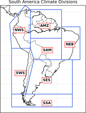
Figure 1. Spatial map showing different climate regions in South America proposed for IPCC AR6 reference regions: Northwest South America (NWS), Amazon (AMZ), South America Monsoon (SAM), Northeast Brazil (NEB), Southwest South America (SWS), Southeast South America (SES), and Southern South America (SSA).
Download figure:
Standard image High-resolution image2.4. Area and population of exposure
The area and population that experience Rx5d events exceeding the threshold for dangerous extreme precipitation (once-in-100 year events) are aggregated spatially to represent the total area and population exposed, weighted by grid box area. Fractional exposure is calculated with respect to the total area or total population within each of the regions defined in figure 1. Population exposures are estimated based on populations from the year 2000 (GPW2000) and those projected under different SSPs to represent possible future socio-economic development scenarios. Population distributions in the year 2000 are from the Gridded Population of the World, version3 (GPWv3, http://sedac.ciesin.columbia.edu/data/set/gpw-v3-population-count). Future population distributions under different SSPs by 2100 are from Jones and O'Neill (2016). The spatial distribution of GPW and different SSPs over South America are shown in figure S1.
3. Results
First we investigate the return times of dangerous extreme precipitation under different warming levels. Figure 2 shows the spatial distribution of the return time of Rx5d at different warming levels associated with the historical 100 year return levels. Red color denotes decreased return time, i.e. such events will happen more frequently in the future; gray color denotes increased return time, i.e. such events will happen less frequently in the future. For each model, the best estimate of the ensemble is shown. All models show dangerous extreme precipitation events have shorter return times, i.e. they happen more frequently with the additional 0.5 °C warming, especially in the NWS, SAM, and SES regions. The models disagree over Northern AMZ and NEB. For the Northern AMZ region, HadAM3P, HadRM3P, MIROC5 and CanAM4 show less frequent occurrence of dangerous extreme precipitation under both warming levels, whereas the other models show more frequent occurrence. For NEB region, HadAM3P, HadRM3P show less frequent occurrence of dangerous extreme precipitation over the northern part, and CanAM4 shows less frequent occurrence over the majority of NEB region, whereas the other models mostly show more frequent occurrence.
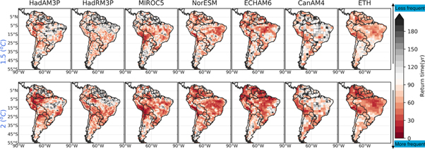
Figure 2. The return time of Rx5d at different warming levels associated with the historical 100 year return levels in 1.5 °C warming world (top row) and in 2 °C warming world (bottom row). Red color means decreased return time, i.e. such events will happen more frequently in the future; gray color means increased return time, i.e. such events will happen less frequently in the future. For each model, the best estimate of the ensemble is shown.
Download figure:
Standard image High-resolution imageFigure 3 shows the results for NEB region after aggregating spatially (results for the other regions are shown in figures S2–S7). The occurrence of the type of events with return level corresponding to the historical 100 year return period, is shown as the horizontal dashed black line in each panel; the 5th–95th percentile ranges of the estimated return time associated with the historical 100 year return levels at different warming levels are shown as the vertically shaded area. All models, with the exception of CanAM4, show shortened return time (with the numbers shown in table 2), i.e. more frequent occurrence of such dangerous extreme precipitation events from historical to 1.5 °C warming and from 1.5 °C to 2 °C warming. Out of these six models, five (HadAM3P, HadRM3P, NorESM, ECHAM6, and ETH-CAM4) show statistically significant shift from 1.5 °C and 2 °C warming, denoted by the non-overlapping shaded uncertainty range in figure 3. The CanAM4 model results present a nonlinear change from historical to 1.5 °C, and from 1.5 °C to 2 °C. Under 1.5 °C, the return time is significantly longer (the lower bound of the uncertainty range is longer than 100 years), whereas under 2 °C, the return time is significantly shorter (the upper bound of the uncertainty range is shorter than 100 years). Such nonlinear response to increasing global mean temperatures in CanAM4 suggests that, there are underlying dynamical changes in play that warrants further investigation. Interestingly, a previous study (Hawkins et al 2014) has also showed that several GCMs from CMIP display evidence of non-monotonic changes for precipitation over tropical South America, with some models suggesting an increase until 2100, followed by a decrease. Although this current paper uses the HAPPI simulations, which is a framework based on global temperature response rather than an emission scenario approach like the CMIP simulations, both modeling approaches show nonlinear change in precipitation over tropical South America. This region plays a disproportionately large role both in hosting biodiversity and affecting global earth system functions, including the global carbon balance, all of which may be affected by changes in precipitation. Therefore, it is of great importance to further investigate the underlying mechanisms and raise awareness of impact modelers, decision makers etc. Because nonlinear changes like this could lead to unexpected impacts in this biodiversity hotspot.
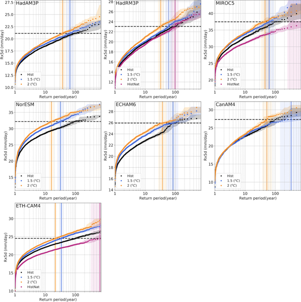
Figure 3. Return levels of Rx5d against their return period are shown, represented by the filled circles in black for historical (Hist), magenta for HistNat (shown for models with available simulations), blue for 1.5 °C warming and orange for 2 °C warmings. Uncertainties are estimated by bootstrap resampling. The shaded area represent the 5%–95% confidence intervals from bootstrapping. The horizontal dashed black lines represent the historical 100 year return levels of the Rx5d events. The vertical solid lines in magenta, blue and orange represent the return periods associated with the historical 100 year return levels under HistNat, 1.5 °C warming and 2 °C warming, respectively, and the shaded area represents the 5%–95% confidence intervals of return period from bootstrapping. The results for the Northeast Brazil (NEB) region are shown here, and the corresponding results for the other climate regions are shown in the supplementary information (figures S2–S7).
Download figure:
Standard image High-resolution imageTable 2. The return periods associated with the historical 100 year return levels of the Rx5d events under the HistNat, 1.5 °C warming and 2 °C warming scenarios in different models, and the numbers in the parenthesis are the 5th–95th percentile ranges corresponding to the vertically shaded area shown in figure 3—the results for Northeast Brazil (NEB) region are shown.
| HistNat | 1.5 °C | 2 °C | |
|---|---|---|---|
| HadAM3P | 65(50, 92) | 38(30, 47) | |
| HadRM3P | 97(72, 135) | 60(45, 78) | 33(26, 41) |
| MIROC5 | 1000 (333, 1000) | 63(43, 100) | 45(33, 67) |
| NorESM | 32(25, 42) | 16(13, 20) | |
| ECHAM6 | 83(53, 143) | 37(27, 50) | |
| CanAM4 | 333(143, 1000) | 53(37, 77) | |
| ETH-CAM4 | 642(321, 1605) | 34(30, 39) | 22(19, 24) |
In the HistNat (counterfactual) simulations, results suggest that without human influences, events like the historical 100 year event would have occurred much less frequently in the MIROC5 and ETH-CAM4 models (as seen from the lengthened return times shown in table 1), but there is no significant change in HadRM3P. Caution needs to be taken if these return time numbers were to be quoted to guide decision making on a regional level, because these climate regions have wide spatial coverages, and there are strong spatial heterogeneity (as seen in figure 2) within regions to take a one-fit-for-all approach.
To make it easier to discuss and summarize changes in likelihood, in figure 4, we present the RRs for the Rx5d events that exceed the historical 100 year return levels under 1.5 °C warming (shown in blue), and under 2 °C warming (shown in orange) for different climate regions, simulated by different models. The horizontal line in each panel denotes the RR of 1 line, and RR above one indicates increased risk, i.e. more frequent occurrence of dangerous extreme precipitation events. In each violin, all the grid points within a region are shown, and for each grid point, the best estimate is shown. Both sides of each violin are rotated kernel density estimates, with thickness indicating frequency/density of grid points, and a standard box plot is drawn inside each violin. Figure 4 echoes our point earlier that there is strong spatial heterogeneity (with RRs ranging from 0 to 10, and above in some cases) within each region, and often times the distribution of RR (denoted by the rotated kernel density estimates in the violin plots) presents a bimodal (e.g. NWS simulated by ECHAM6) or tri-modal (e.g. SSA simulated by CanAM4) shape. For most cases, over 50% of the region experiences increased likelihood of extreme precipitation under future warming. These violin plots highlights the fact that it could be misleading to just look at distributions from the standard box plots, because the peak density/frequency of RRs within a region does not necessarily coincide with the median or mean of the distribution, especially in regions where heterogeneous RRs are present (e.g. NWS region the HadAM3P model result under 2 °C warming and SWS region the ECHAM6 model results). The RRs for each country are shown in figure S8.
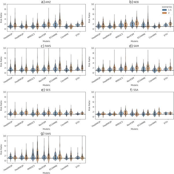
Figure 4. The risk ratios for the Rx5d events that exceed the historical 100 year return levels under 1.5 °C warming (shown in blue), and under 2 °C warming (shown in orange) are shown for different climate regions, simulated by different models. Both sides of each violin are rotated kernel density estimates, with thickness indicating frequency, and a standard box plot is drawn inside each violin. In each violin, all the grid points within a region are shown, and for each grid point, the best estimate is shown. The horizontal line in each panel denotes the RR = 1.
Download figure:
Standard image High-resolution imageTo summarize the avoided area of exposure to the increased risk of more frequent dangerous extreme precipitation events, simulated by all the models, figure 5 shows the avoided area of exposure (%) by limiting to 1.5 °C warming (compared with 2 °C warming) for the Rx5d events that exceed the historical 100 year return levels for different climate regions in panel (a), and different countries in panel (b). Circles and bars denote multi-model medians and ranges, respectively. Where more (less) than 4/7 of the models indicate avoided exposure by limiting to 1.5 °C warming are indicated by solid (open) circles. There is model agreement (>=5/7) in all regions and all countries (except Guyana and Suriname) that less area would be exposed to more frequent dangerous extreme precipitation events by limiting to 1.5 °C warming level, although the percentage of the avoided area of exposure varies. SES shows the highest multi-model median percentage (13.3%) of avoided exposure of all regions and SWS shows the lowest percentage (3.1%). Of all countries, Ecuador shows the highest multi-model median percentage (17%) of avoided exposure, whereas Guyana and Suriname show almost no change in the multi-model median result.
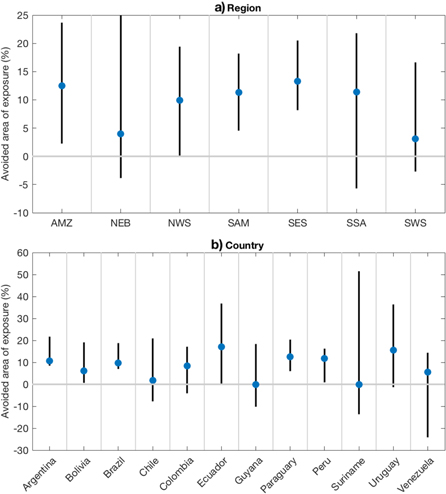
Figure 5. Avoided area of exposure (%) by limiting to 1.5 °C warming (compared with 2 °C warming) for the Rx5d events that exceed the historical 100 year return levels for (a) different climate regions, and (b) different countries. Circles and bars denote multi-model medians and ranges, respectively. Where more (less) than 4/7 of the models show avoided exposure by limiting to 1.5 °C warming are indicated by solid(open) circles.
Download figure:
Standard image High-resolution image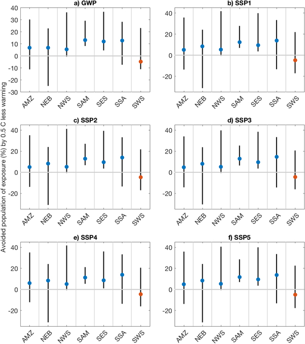
Figure 6. Avoided population of exposure (%) by limiting to 1.5 °C warming (compared with 2 °C warming) for the Rx5d events that exceed the historical 100 year return levels, for different climate regions under population distribution fixed at the year 2000 (Gridded Population of the World, GPW) in (a), and under different Shared Socioeconomic Pathways (SSPs) 1–5 in (b)–(f). Circles and bars denote multi-model medians and ranges, respectively. Where more (less) than 4/7 of the models show avoided exposure by limiting to 1.5 °C warming are indicated by solid(open) blue circles, and where more than 4/7 of the models show increased exposure by limiting to 1.5 °C warming are indicated by solid orange circles.
Download figure:
Standard image High-resolution image
Under all SSPs, in NWS, SAM and SES, the impact of limiting to 1.5 °C shows a definite decrease in exposure for those areas (figure 6). Furthermore, across all the regions, the multi-model median effect is a decrease in population exposure (an increase in avoided exposure) by limiting warming to 1.5 °C, apart from the mountainous SWS region where there is a small increased exposure. Although uncertainty ranges for SWS still show that a big proportion of the model spread is on the decreased exposure side. We find that the exposure avoided is very similar under different SSP scenarios (figure 6), indicating that in the case of extreme precipitation impacts, the change in hazard plays an important role in future risks compared with population changes. However, model representation of mountainous regions such as SWS may be poorly represented due to resolution constraints (Leung et al 2003a, 2003b), and climate models tend to have difficulties correctly representing precipitation correctly over regions with strong topographic gradient such as the Andes regions (e.g. Solman et al 2008). Therefore, the results over SWS warrant further investigation.
4. Summary and discussions
The overarching finding of this study is that the likelihood of dangerous extreme precipitation increases in large parts of South America under future warming, and that overall more warming leads to more extreme precipitation. What this study however particularly highlights is that (1) for most regions the increase is rather heterogeneous even within a climate region that has been chosen to represent a similar climate, (2) that the changes in likelihood as well as the spatial heterogeneity are relatively similar across models, and (3) that changes in extreme precipitation are nonlinear with increasing global mean temperatures.
All these findings are potentially highly valuable for local and regional decision making and our analysis underlines the need for spatially explicit information on the resolutions presented here, or higher, as crucial for designing adaptation strategies. There is good model agreement in terms of the future projected change of extreme precipitation due to increased global warming across many regions with the exception of northern AMZ and NEB . However, the fact that we see a different change in the likelihood of extreme precipitation between the pre-industrial simulations (−1° from the present) compared to the 2 °C scenarios (+1° from the present) indicates that the response to increased greenhouse gases emissions are nonlinear for each degree of additional warming. This in turn suggests that various feedback processes may be taking place or drivers other than greenhouse gases play an important role. Also the response within a single region can be complex such as in the AMZ region, where not only do models show less agreement, there is also stronger spatial variation within the region in terms of the direction of change in response to warming, with some models (NorESM, ECHAM6, and ETH) showing enhanced frequency of extreme precipitation throughout the region, while others showing mixed signals across the region. The spatially incoherent signal in the northern AMZ and NEB regions also suggests it is important to investigate the dynamical drivers behind the projected changes as seen here in future research.
The large model uncertainty shown in the projected changes in extreme precipitation over the northern AMZ and NEB is consistent with the findings of previous studies (e.g Knutti and Sedláček 2013, McSweeney and Jones 2013): despite strong model agreement for large-scale circulation change (e.g. weakening of the tropical circulation, and expansion of the Hadley cell), which are robust across CMIP3 and CMIP5 ensembles (Christensen et al 2013, Chadwick et al 2013, DiNezio et al 2013, Ma and Xie 2013, Chadwick et al 2014), climate model agreement for projected precipitation change is lower in the tropics, with model disagreement on even the sign of change over large areas. To understand uncertainty in tropical precipitation projections, Chadwick et al (2013) assessed the driving mechanisms behind tropical precipitation pattern changes in CMIP5 projections, and showed that the spatial patterns of the thermodynamic change due to increased atmospheric water vapor (i.e. wet-get-wetter) and the decreased convective flux due to the weakening tropical circulation cancel each other out to a large extent, which leave the spatial pattern of precipitation change to be dominated by shifts in the convection and convergence zones. For daily regional scale extreme precipitation, Pfahl et al (2017) found that dynamic contribution is key to the uncertainty in future projected changes of regional extreme precipitation. Of the CMIP5 models Chadwick et al (2013) used, four models have corresponding atmospheric-models (CanAM4, MIROC5, NorESM1, and HadAM3P) in the HAPPI simulations used in this study; while of the CMIP5 models used in Pfahl et al (2017), three have corresponding atmospheric-models (CanAM4, MIROC5, and NorESM1) in HAPPI. Although beyond the scope of this study, an interesting next step would be to assess the driving mechanisms behind the projected changes in extreme precipitation over the tropical South America in all the HAPPI models, to better understand model uncertainty in tropical precipitation projections.
We also find that the exposure avoided is very similar in different SSP scenarios (figure 6), indicating that in the case of dangerous extreme precipitation impacts, population changes play less of an important role, whereas the change in the hazard plays a more dominant role in future risks.
To conclude, limiting warming to 1.5 °C as opposed to 2 °C shows a general reduction in both area and population exposure to dangerous extreme precipitation throughout South America, with SES shows the highest multi-model median percentage of avoided area exposure at 13.3% and SWS region shows the lowest percentage at 3.1%. While under all SSPs, SAM and SSA regions show the highest multi-model median percentage of avoided population exposure (>10%). Within each climate region and country, the projected changes in risks of dangerous extreme precipitation occurring in all the models show strong spatial heterogeneity.
Risk is determined not only by climate and weather events (hazards), but also by the exposure and vulnerability to the hazards (Lavell et al 2012). Identifying vulnerable populations and factors that contribute to their vulnerability are crucial, because social vulnerability influences the ability to respond to, cope with, and recover from a natural disaster (Aksha et al 2019). However, social vulnerability is highly context-specific, and in contrast to exposure data not meaningfully assessed on a continental scale. Our results nevertheless underscore the importance of incorporating location-specific information about changing climate hazards when designing adaptation measures and investing in disaster preparedness.
Acknowledgments
This research is supported by the Nature Conservancy-Oxford Martin School Climate Partnership. This research used science gateway resources of the National Energy Research Scientific Computing Center, a DOE Office of Science User Facility supported by the Office of Science of the US Department of Energy under Contract No. DE-AC02-05CH11231. We would like to thank our colleagues at the Oxford eResearch Centre for their technical expertise and the available code provided in the CPDN-Git GitHub repositories. We would also like to thank the Met Office Hadley Centre PRECIS team for their technical and scientific support for the development and application of weather@Home. Finally, we would like to thank all of the volunteers who have donated their computing time to climateprediction.net and weather@home.
Data availability
The model data (from MIROC5, NorESM, ECHAM6, CanAM4, ETH) that support the findings of this study are openly available at https://portal.nersc.gov/c20c/data/. The rest of the modeled data that support the findings of this study are available from the corresponding author upon reasonable request. European Centre for Medium-Range Weather Forecasts' ERA5 and ERA-Interim data products are openly available from the Copernicus Climate Change Service (C3S) at https://cds.climate.copernicus.eu/. CPC, GPCC, and GPCP dataset are provided by the NOAA/OAR/ESRL PSD, Boulder, Colorado, USA, from their website at https://esrl.noaa.gov/psd/. CHIRPS dataset is obtained from the Climate Hazards Center, UC Santa Barbara, from their website at https://chc.ucsb.edu/data/chirps.