


Abstract
The Arctic is warming twice as fast as the rest of the planet, leading to rapid changes in species composition and plant functional trait variation. Landscape-level maps of vegetation composition and trait distributions are required to expand spatially-limited plot studies, overcome sampling biases associated with the most accessible research areas, and create baselines from which to monitor environmental change. Unmanned aerial vehicles (UAVs) have emerged as a low-cost method to generate high-resolution imagery and bridge the gap between fine-scale field studies and lower resolution satellite analyses. Here we used field spectroscopy data (400–2500 nm) and UAV multispectral imagery to test spectral methods of species identification and plant water and chemistry retrieval near Longyearbyen, Svalbard. Using the field spectroscopy data and Random Forest analysis, we were able to distinguish eight common High Arctic plant tundra species with 74% accuracy. Using partial least squares regression (PLSR), we were able to predict corresponding water, nitrogen, phosphorus and C:N values (r2 = 0.61–0.88, RMSEmean = 12%–64%). We developed analogous models using UAV imagery (five bands: Blue, Green, Red, Red Edge and Near-Infrared) and scaled up the results across a 450 m long nutrient gradient located underneath a seabird colony. At the UAV level, we were able to map three plant functional groups (mosses, graminoids and dwarf shrubs) at 72% accuracy and generate maps of plant chemistry. Our maps show a clear marine-derived fertility gradient, mediated by geomorphology. We used the UAV results to explore two methods of upscaling plant water content to the wider landscape using Sentinel-2A imagery. Our results are pertinent for high resolution, low-cost mapping of the Arctic.
Export citation and abstract BibTeX RIS

Original content from this work may be used under the terms of the Creative Commons Attribution 4.0 license. Any further distribution of this work must maintain attribution to the author(s) and the title of the work, journal citation and DOI.
1. Introduction
The Arctic is the fastest warming region on earth [1]. Air temperatures have risen at twice the global rate [2], driving changes to the structure and functioning of tundra ecosystems [3–7]. Increased temperatures lead to shifts in vegetation cover and composition and accelerate belowground nutrient cycling and mineralization rates, with potentially important effects on global climate [8–14].
Plant traits are a primary control on the distribution and functioning of plants and underpin vegetation–climate responses (e.g. [15–17]). Traits related to the uptake and allocation of resources, such as leaf mass per area, leaf water content, leaf nitrogen content (N) and leaf phosphorus content (P) can affect growth rates, plant longevity, primary productivity, decomposition rates and biogeochemical cycling [18–22]. Simultaneously, morphology-related traits, such as leaf area and plant height, can influence aboveground biomass, surface albedo and snow dynamics [14, 23, 24]. Establishing spatial environmental–trait relationships could provide a quantitative basis to forecast the effects of climate change in the Arctic [25, 26]. Yet observational plot-studies often fail to isolate environmental drivers or take place at a smaller scale than the community/landscape they represent. Hence, the biotic consequences of warming in the coldest environments remain poorly predicted [27].
When variations in vegetation characteristics affect spectral reflectance, these changes can be measured using optical remote sensing techniques. In comparison to traditional field-based methods, using remote sensing to generate vegetation data is less laborious, less invasive, more cost-effective and spatially continuous. Using multispectral satellite-based sensors, the distribution of Arctic vegetation has been well-established at broad scales through datasets such as the Circumpolar Arctic Vegetation Map (CAVM [28]), which classifies 16 Arctic vegetation types at 1 km resolution. Using coarse-resolution satellite imagery, widespread vegetation change at high latitudes has also been well-documented, including pan-Arctic 'greening' and 'browning' trends [29–32], with important implications for albedo, active layer depth, permafrost dynamics, carbon cycling and wildlife [10, 33–41]. However, vegetation cover in the Arctic is extremely heterogeneous, varying at very fine spatial scales ([42–44]), and observations do not always agree at the satellite and plot level [32, 45, 46]. Thus, while remote sensing offers enormous potential to generate large-scale vegetation data across the Arctic, such coarse spatial and spectral resolution is limited in its ability to capture the fine-scale dynamics of tundra plants or resolve the key drivers of observed vegetation trends [32, 47, 48].
In lower-latitude environments, high-resolution field spectroscopy (visible-near infrared (VNIR: 400–1100)) or visible-short-wave infrared (VSWIR: 400–2500 nm) is a well-established technique for gathering plant taxonomic and trait data with a high degree of accuracy [49–52]. Specific spectral reflectance and absorption features have been directly linked to concentrations of cellulose, lignin, chlorophyll, nutrients and water (see [53] for a comprehensive synthesis). These plant traits can be combined to create unique chemical 'fingerprints' to distinguish individual genera or species [54–57]. Compared to multispectral remote sensing, field spectroscopy provides numerous spectral bands that can capture fine-scale spectral differences and improve discrimination of vegetation features. Spectroscopy studies are rarely extended to the tundra however, likely due to the challenging logistics and the fact that field spectrometers are not designed to accommodate the small size of tundra plant leaves. Spectroscopy studies carried out in the Arctic have mainly focused on classifying tundra communities [58–62], vegetation cover fraction [63], biophysical plant traits, such as vegetation height and biomass [61, 64], and leaf chlorophyll content or 'greenness' [61, 65], but not individual species or plant chemical traits. Remote sensing of high-latitude vegetation would benefit from more spectroscopy studies, which can link plant characteristics to spectral features at specific wavelengths, as well as establish remote sensing baselines (i.e. if a vegetation characteristic cannot be determined using field spectroscopy, it is unlikely to be distinguished using coarser spatial and spectral resolution imagery).
By itself however, spectroscopy cannot generate the spatial and temporal data required to map and monitor biotic change in the Arctic. In order to bridge this 'scale-gap', unmanned aerial vehicles (UAVs) have emerged as platforms to upscale field data and provide nuance to satellite observations [47, 48, 66]. Due to the miniaturization of technology and decreasing costs, UAV-mounted sensors can facilitate the mapping and monitoring of vegetation at previously unachievable spatial, spectral and temporal resolutions. Using hyper and multispectral imagery, UAVs have been used to map plant communities [67, 68], individual species [69–71], plant traits [72–74] and plant health [69, 75–77]. While some UAV studies have applied structure-from-motion methods to analyse biophysical plant characteristics in the Arctic (e.g. [78, 79]), or applied spectral techniques to classify high latitude plant communities (e.g. [59, 67, 68, 80]), to the best of our knowledge, this is the first study to use field spectroscopy and UAVs to identify high Arctic plant species and map vegetation chemistry across the tundra.
In this study, we investigate the use of field spectroscopy for predicting species identity and retrieving plant water and chemistry concentrations across a range of common species at three sites found near Longyearbyen, Svalbard. Based on the demonstrated feasibility of generating plant taxonomic and trait data using field spectra, we develop analogous models using UAV five-band multispectral imagery. Additionally, we explore methods of upscaling our UAV results to the wider landscape using Sentinel-2A imagery. Specifically, we aim to:
- (a)develop predictive models of species identity and biochemical plant traits (water, nitrogen, phosphorus and C:N concentrations) using field spectroscopy,
- (b)develop predictive models of species identity and the same plant traits using UAV spectra,
- (c)apply the UAV models to UAV imagery to derive spatially continuous maps of plant species and their corresponding trait values,
- (d)explore two methods of upscaling the UAV models to the wider landscape using Sentinel-2A imagery.
2. Methods
2.1. Study sites
The data were collected at three High Arctic study sites around Longyearbyen on the Svalbard Archipelago, Norway (figure 1). The sites comprised two contrasting environmental gradients and an experimental warming site. The sites are characterized by a dry Arctic climate with a mean average temperature of −2.6 °C and an average maximum and minimum monthly temperature of 7.6 °C and −11.4 °C (2005–2018). Precipitation is around 190 mm per year (all data obtained from the National Center of Environmental Information [81]). In all cases, underlying soils were typical cryosols with a thin organic layer on top of inorganic sediments [82].

Figure 1. (a) Map of Svalbard archipelago. (b) Map of study sites near Longyearbyen, Svalbard. Basemaps are from the Norwegian Polar Institute. Coordinates in UTM Zone 33 N, WGS84 ellipsoid.
Download figure:
Standard image High-resolution image2.1.1. The Birdcliffs (78.14° N, 15.2° E)
Located near Bjørndalen, up the slope of Platåfjellet, the Birdcliffs is a 175 m high, 450 m long nutrient and elevation gradient, stretching from the base of a Little Auk (Alle alle) and Black-legged Kittiwake (Rissa tridactyla) colony to sea level at Isfjorden. The top of the gradient receives high nutrient input in the form of bird guano and other associated biological material [83]. The majority of the site is characterised by steep slopes and large alluvial fans made up of a mix unconsolidated material of various sizes. Vegetation is dominated by dry dwarf shrub tundra in topographically elevated areas, particularly Salix polaris and Dryas octopetala. Mosses and graminoids dominate in moist areas, especially around the edge of the alluvial fans and towards the flatter end of the gradient near the shore.
2.1.2. The control gradient (78.12° N, 15.4° E)
The Control Gradient is an 850 m long colluvial slope located up the north face of Lindholmhøgda, a spur at the mouth of the Adventdalen valley. The gradient runs from 200 m.a.s.l to a reservoir (Isdammen) at sea level. The area is characterised by dry dwarf shrub tundra that alternates with ridge communities of scarce vegetation. Habitats with thin winter snow cover are dominated by Dryas octopetala and Salix polaris (Dryas heath), while habitats of intermediate snow depth are dominated by Cassiope tetragona (Cassiope heath).
2.1.3. The international tundra experiment (78.18° N, 15.77° E)
The International Tundra Experiment (ITEX [84]) is an experimental warming site located in Endalen. Data were collected outside the warming chambers from three predominant habitats: an exposed and relatively dry Dryas heath with shallow snow cover in winter, a mesic Cassiope heath with intermediate winter snow depth and a moist snowbed community dominated by bryophytes, Salix polaris, Bistorta vivipara and graminoids.
2.2. UAV imagery acquisition
All fieldwork was conducted as part of the Plant Functional Trait Course 4 (https://plantfunctionaltraitscourses.w.uib.no/), from 16 July 2018 to 27 July 2018. See figure 2 for a diagrammatic representation of the data collection and analysis.
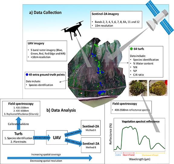
Figure 2. Diagrammatic representation of (a) the data collection and (b) the data analysis. Only the Birdcliffs site is shown here. Further turfs, ground-truth points and UAV imagery were collected at the Control Gradient and ITEX site.
Download figure:
Standard image High-resolution imageUAV imaging data were acquired from all three sites. The data were acquired using a 3DR Solo drone equipped with a MicaSense RedEdge-MX multispectral camera and MicaSense RedEdge Downwelling Light Sensor (DLS). The MicaSense RedEdge–MX camera captures surface reflectance at five narrow spectral bands: blue (475 nm), green (560 nm), red (668 nm), Red Edge (717 nm) and NIR (840 nm). The DLS points upwards and captures illumination conditions, which are embedded in the metadata of each image. The drone was flown at an altitude of 40–60 m, resulting in <10 cm resolution imagery. To map the entirety of the study sites, multiple overlapping flights were required, which were taken over the course of one day at each site. Radiometric calibration images were recorded using a MicaSense reflectance panel as the calibration target. Ground control points for georeferencing were taken using the Emlid Reach+ differential GNSS system (Emlid, Hong Kong).
The imagery was processed in Pix4Dmapper (v.4.3.31, Pix4D, Lausanne, Switzerland) using a standard structure-from-motion (SfM) workflow. For each site, images from all flights were processed in the same project to form a single orthomosaic. The GCPs were manually identified in the images and georeferenced using their field-collected RTK–GNSS coordinates. Across the three sites, this resulted in RMS errors of 0.10–0.14 m. Radiometric calibration was performed in Pix4D using the MicaSense reflectance target images and the metadata from the DLS.
2.3. Vegetation sampling
After the UAV imagery acquisition, 68 20 × 20 cm single-species turfs were collected from across the Birdcliffs and ITEX sites. The turfs were selected to represent the most common plant functional types identified across all sites: mosses, graminoids and dwarf shrubs (table 1, figure 2). High-accuracy GNSS coordinates were taken from the locations of the extracted turfs with an Emlid Reach+ differential GNSS system. Additional vegetation ground-truthing points were taken from all three sites (table 2, figure 2). The turfs were cut to a substrate depth of approximately 5 cm, sealed inside plastic bags and transported back to the University Centre in Svalbard (UNIS) for species identification and analysis.
Table 1. Information on turf samples, including site location, plant functional type, genus and species. Turfs measured 20 × 20 cm. Five independent spectrum readings were taken per turf.
| Turf samples | |||||
|---|---|---|---|---|---|
| Site | Plant functional type | Genus | Species | N. of turf samples | N. of Spectra |
| Birdcliffs | Moss | Aulacomnium | Palustre | 3 | 15 |
| Aulacomnium | Turgidum | 4 | 20 | ||
| Polytrichastrum | Alpinum | 2 | 10 | ||
| Polytrichum | Hyperboreum | 1 | 5 | ||
| Polytrichum | Strictum | 1 | 5 | ||
| Racomitrium | Canescens | 2 | 10 | ||
| Racomitrium | Lanuginosum | 2 | 10 | ||
| Birdcliffs | Graminoid | Alopecurus | Ovatus | 7 | 35 |
| Luzula | Confusa | 6 | 30 | ||
| Luzula | Nivalis | 1 | 5 | ||
| Birdcliffs | Dwarf shrub | Cassiope | Tetragona | 2 | 10 |
| Dryas | Octopetala | 5 | 25 | ||
| Salix | Polaris | 9 | 45 | ||
| ITEX | Moss | Identity not recorded | 5 | 25 | |
| ITEX | Graminoid | Identity not recorded | 1 | 5 | |
| ITEX | Dwarf shrub | Cassiope | Tetragona | 2 | 10 |
| Dwarf Shrub | Dryas | Octopetala | 3 | 15 | |
| Dwarf Shrub | Salix | Polaris | 3 | 15 | |
| Senesced Shrub | Cassiope | Tetragona | 6 | 30 | |
| Senesced Shrub | Dryas | Octopetala | 3 | 15 | |
| Total: 68 | Total: 340 | ||||
Table 2. Information on ground-truthing vegetation survey, including site, plant functional type and number of data points. GNSS locations were taken with an Emlid Reach+ differential GNSS.
| Ground-truthing vegetation survey | ||
|---|---|---|
| Site | Plant functional type | N. data points |
| Birdcliffs | Moss | 15 |
| Graminoid | 23 | |
| Dwarf Shrub | 24 | |
| Control Gradient | Moss | 9 |
| Graminoid | 0 | |
| Dwarf shrub | 9 | |
| ITEX | Moss | 6 |
| Graminoid | 1 | |
| Dwarf shrub | 30 | |
| Total: 117 | ||
Some shrub samples collected from the dry and mesic heaths at ITEX showed signs of tissue degradation, probably due to drought or frost damage [85]. These samples were included in the plant trait analyses, as part of a continuum of trait values, but excluded from the species classification analyses. Mapping plant health falls outside the scope of this study and only healthy shrub communities were observed over the UAV upscaling areas.
2.3.1. Field spectroscopy measurements
Field spectroscopy measurements of the turf samples (350–2500 nm) were taken at UNIS using an ASD Fieldspec Pro with fibre optic cable and contact probe (Analytical Spectral Devices, Boulder, CO, USA). Turfs were stored outside and reflectance measurements were taken within 24 h of turf cutting. Spectroscopy measurements were not taken 'in situ' at study sites, due to the non-portable set-up of the spectrometer. Turfs were selected to be as homogenous as possible. If multiple plant species were present across the turf, measurements were only taken from areas where the main species dominated. The contact probe was pushed firmly down onto the turf so all extraneous light was excluded from the measurement. Five measurements were taken at different locations across each turf. Each measurement consisted of 40 internally averaged reflectance readings to increase the signal-to-noise ratio. The spectrometer was optimised and calibrated for dark current and white light after every turf. For all statistical analyses, the spectral data were trimmed to the 400–2500 nm range. For some analyses, the five measurements were averaged to form one spectrum per turf.
2.3.2. Plant trait sampling
After the field spectroscopy measurements had been taken, three 5 × 5 cm vegetation samples were cut from each turf. For each sample, all vegetation above the substrate was harvested. The samples were weighed for fresh mass, dried at 60 °C for 48 h and re-weighed for dry mass. Vegetation water content was calculated as ((fresh mass − dry mass)/fresh mass) × 100.
Nutrient analysis of the dried samples was carried out at the University of Arizona. The protocol to obtain total phosphorus concentration involved using persulfate oxidation followed by the acid molybdate method (APHA, 1992), after which P concentration was determined via colorimetric analysis with a spectrophotometer (ThermoScientific Genesys20, United States). Carbon, nitrogen, and their stable isotope ratios were measured at the Department of Geosciences Environmental Isotope Laboratory on a continuous-flow gas-ratio mass spectrometer.
The three samples were averaged to form one trait value per turf. See table S1 (available online at stacks.iop.org/ERL/16/055006/mmedia) for average trait values.
2.4. Field spectroscopy analyses
2.4.1. Field spectroscopy-species analysis
The turf spectra were divided into eight vegetation classes (below) representing a mixture of families, genera and species. Some of the moss and graminoid species were combined into their families or genera to increase the class sample size and because they were assumed to be spectrally similar. Mosses were classified into Aulacomnium spp. (containing Aulacomnium palustre and Aulacomnium turgidum); Polytrichaceae spp. (containing Polytrichum hyperboreum, Polytrichastrum alpinum and Polytrichastrum strictum); and Racomitrium spp. (containing Racomitrium canescens and Racomitrium lanuginosum). The graminoids were classified into Alopecurus ovatus (a grass) and Luzula spp. (a rush, containing Luzula confusa and Luzula nivalis). The dwarf shrubs were separated into Cassiope tetragona, Dryas octopetala and Salix polaris.
To quantify similarity or differences between the spectra, agglomerative hierarchical cluster analysis was performed using the eight classes described above and one averaged spectrum per turf. Cluster analysis works by calculating the distance (difference) between each possible pair of spectra. The two spectra closest to each other are merged and the process repeats, with the number of clusters reduced by one each cycle. Spectral distances were calculated using Euclidean Distance in MATLAB (MathWorks, Natick, MA, USA).
The eight vegetation classes were predicted using five spectra per turf and Random Forest classification [86]. The five spectra per turf were used as independent samples, as the spectral curves were highly diverse due to the heterogeneous nature of the turfs. Random Forest is a machine learning classifier that grows as an ensemble of decision trees [87, 88]. It is useful for classifying hyperspectral data as it is robust against overfitting and can be used when the number of predictor variables (e.g. 2150 wavelength bands) is greater than the number of samples (e.g. 470 spectra). All the Random Forest analyses were carried out in MATLAB using the Treebagger function.
2.4.2. Field spectroscopy-trait analysis
Plant water, nitrogen, phosphorous and C:N values were predicted using one averaged spectrum per turf and partial least squares regression (PLSR [89]). The PLSR method is effective, as it uses the continuous spectrum as a single measurement, rather than carrying out a band-by-band analysis and reduces a large predictor matrix (2150 spectral bands) down to a few relatively uncorrelated factors (known as latent variables). For the trait predictions, we chose to use PLSR instead of Random Forest Regression because, unlike Random Forest Regression, PLSR is able to extrapolate beyond its calibration data. While Random Forest is a strong tool for classification, it cannot predict values outside of its training range, limiting its accuracy when scaling up continuous data over wider areas that may contain trait values outside the range of the sample data.
PLSR analyses were carried out using the PLSregress function in MATLAB. The PLSR models were validated using an unseen 30% of the dataset. Due to the random nature of the 70:30 split, 1000 PLSR iterations were made for each spectra-trait analysis. The PLSR equations resulting in robust models (r2 > the mean value of the 1000 iterations) were evaluated using r2 for the independent testing (val) dataset and RMSE as a percentage of the sample mean (as in [90, 91]).
All Random Forest and PLSR analyses were carried out using (a) the full hyperspectral range from 400 to 2500 nm, (b) just the VIS–NIR region from 400 to 1000 nm and (c) downscaled spectra to match the five bands represented by the MicaSense camera (blue, green, red, red edge and near-infrared). The three analyses were carried out in order to act as a baseline from which the effects of decreased spectral information and the effects of using an airborne camera could be accurately separated.
2.5. UAV spectral analysis
2.5.1. UAV spectra-species analysis
UAV spectra were extracted from the orthomosaic at all the points where the turfs and ground-truthed species coordinates were taken. The spectra were extracted using the 'extract' function in the Raster package [92] in R (v.3.6.0, R Core Team, 2019). First, an NDVI mask was applied to the imagery to mask out any pixels with an NDVI of <0.5. The threshold of 0.5 was chosen as it represents the lower limit of NDVI values measured for vegetation in the Arctic [93]. The UAV spectra were extracted using three methods: simple (only the pixel value the coordinate falls in is returned), bilinear (the returned value is interpolated from the values of the four nearest pixels) and buffer (the returned value is averaged from all the pixels that fall within a specified 3 × 3 pixel buffer area). Across all analyses, the buffer method demonstrated the most robust results, hence only the results from these analyses are shown.
Using the UAV spectra, Random Forest classification was used to predict three broad plant functional groups: mosses, graminoids and dwarf shrubs. These plant functional groups represented the finest classification of vegetation that could be achieved using the UAV data and the Random Forest method of prediction. The Random Forest model that demonstrated the best result on the training/validation data was scaled up and applied to each pixel of the Birdcliff imagery to generate a continuous ecosystem map of plant functional type. The models were only applied to the Birdcliff site, as this was where the majority of the turfs were collected. As such, we only had confidence in the model validation for the species and environmental conditions found at this site.
2.5.2. UAV spectra-trait analysis
Trait values were predicted using the same UAV spectra and PLSR method described above. The PLSR model that maximised the r2 and minimised the %RMSE was chosen and applied to each pixel of the UAV imagery to generate continuous maps of trait information. Trait values were also compared to an NDVI map generated from the UAV imagery to quantify the benefits of using a multispectral machine learning approach to trait prediction, compared to an NDVI-based prediction (figure S3).
2.6. Sentinel-2A scaling analysis
Sentinel-2A imagery was used to explore methods of upscaling the UAV maps to the wider region. Plant water content was chosen as an example trait, as water has a strong direct expression in spectra and the Birdcliff site was assumed to be a nutrient anomaly in the landscape.
The Sentinel image used in the analysis was a Level-2A cloud-free, atmospherically-corrected image taken on 30th July 2018, one week after the field-collection. Only vegetation pixels were included in the analysis, identified using the Sentinel-2 scene classification layer (SCL). Analyses were carried out in R (v.3.6.0, R Core Team, 2019) and Google Earth Engine (https://earthengine.google.org/).
Two methods of upscaling from UAV to satellite data were tested:
- (a)the UAV-generated map of plant water content (figure 8) was resampled to match Sentinel-2A resolution (10 m) and gridlines using bilinear interpolation. Lower-resolution Sentinel bands were also resampled to 10 m using bilinear interpolation. The resampled UAV water values were used as a calibration and validation dataset for the Sentinel imagery. Thus, each Sentinel pixel (n = 329) had a single water value as well as a reflectance value for each relevant Sentinel band (Band 2 (492 nm), 3 (560 nm), 4 (665 nm), 5 (704 nm), 6 (741 nm), 7 (783 nm), 8 (833 nm), 8A (865 nm), 11 (1614 nm) and 12 (2202 nm)). Using this dataset and the same PLSR method described above, model coefficients were generated for each Sentinel band and applied to each pixel of the Sentinel image.
- (b)the coefficients from the PLSR model used to create the UAV map of water content were applied to the Sentinel bands that best matched the MicaSense bands (Sentinel bands 2,3,4,5 and 8) for each pixel of the Sentinel image.
3. Results
3.1. Field spectroscopy identification of plant functional types and species
Average reflectance spectra for three plant functional types (moss, graminoids and dwarf shrubs) showed distinct spectral separability, especially in the NIR (750–1300 nm) and SWIR regions (1500–2500 nm, figure 3(a)). Moss displayed the lowest reflectance across the NIR–SWIR region, especially in the water absorption bands near 1450, 1940 and 2500 nm [53]. Within each plant functional type, unique spectral signatures were displayed by genera and species (figures 3(b)–(d)). Shrubs were more spectrally similar to each other, but showed some divergence in the NIR–SWIR. Intraspecific spectral variability was low across most of the mosses, while Alopecurus ovatus and Cassiope tetragona displayed the highest spectral variability, especially across the NIR.

Figure 3. Mean (±standard deviation) of turf spectral reflectance (400–2500 nm). Reflectance was measured using an ASD Fieldspec Pro with fibre optic cable and contact probe. (a) Spectra were grouped into three plant functional types; mosses, graminoids and dwarf shrubs. The MicaSense RedEdge-MX five spectral bands (blue, green, red, red edge and near–infrared) are shown in grey for comparison purposes. (b) Mosses were classified into Aulacomnium spp. (A. palustre and A turgidum), Polytrichaceae spp. (P. hyperboreum, P. alpinum and P. strictum), and Racomitrium spp. (R. canescens and R. lanuginosum). (c) Graminoids were classified into Alopecurus ovatus and Luzula spp. (L. confusa and L. nivalis). (d) Shrubs were separated into C. tetragona, D. octopetala and S. polaris.
Download figure:
Standard image High-resolution imageUsing cluster analysis to further quantify spectral separability, mosses emerged as a distinct spectral family (figure 4). All moss spectra clustered together, with some stratification of genera, especially Aulacomnium and Racomitrium. There was less guild clustering of graminoids and shrubs, however Salix polaris emerged as a tight cluster and most Dryas octopetala spectra clustered together. Despite some grouping of Luzula, the graminoids did not cluster together as a functional group. The majority of the spectral confusion was created by Alopecurus ovatus and Cassiope tetragona, whose high spectral variability meant they were commonly paired with other shrub and graminoid species.
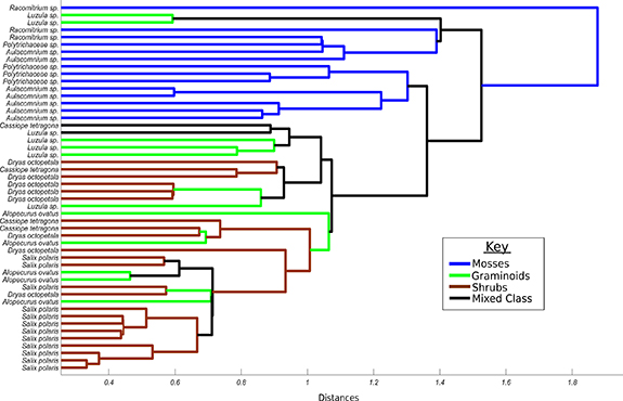
Figure 4. Results of spectral agglomerative hierarchical cluster analysis. One average spectrum per turf was used (n = 53). Spectra are labelled according to the eight vegetative classes described in figure 3 and coloured according to plant functional type (moss, graminoid, dwarf shrub).
Download figure:
Standard image High-resolution imageUsing Random Forest Classification and the full hyperspectral range (400–2500 nm), our results show that eight common Arctic tundra species can be classified with 74% accuracy (much above the expected statistical random accuracy value of 12.5%, given eight classes, figure 5). Reflecting the results of the cluster analysis, moss species displayed the highest classification accuracy values (85, 80 and 80%), along with Salix polaris (80%) and Luzula sp. (80%). Reducing the amount of spectral information led to a small decrease in accuracy to 69 and 66% for the 400–1000 nm spectral range and downscaled MicaSense bands, respectively. Across the eight classes, the greatest source of uncertainty came from the classification of Cassiope tetragona and Dryas octopetala, which were commonly confused with each other (see figure S1 for confusion matrices).

Figure 5. Percentage of turf spectra correctly classified using Random Forest classification. Five spectra per turf were used (n = 265). The spectra were classified three times: (1) using the full hyperspectral range from 400 to 2500 nm, (2) just the VIS–NIR region from 400 to 1000 nm and (3) downscaled spectra to match the five bands represented by the MicaSense-MX camera (blue, green, red, red edge and near-infrared).
Download figure:
Standard image High-resolution image3.2. Field spectroscopy identification of plant traits
Using the full reflectance spectra (400–2500 nm), PLSR results show that plant water content was estimated with the highest accuracy (r2 = 0.88, RMSE = 12%), followed by N (r2 = 0.77, RMSE = 28%), P (r2 = 0.67, RMSE = 64%) and C:N ratios (r2 = 0.61, RMSE = 37%, figure 6(a)). Removing spectral information from the SWIR range had the greatest impact on water prediction. Decreased SWIR spectral information had almost no impact on N prediction, and little impact on C:N ratio prediction. P estimation showed little change with reduced SWIR information but was strongly influenced by fewer VIS–NIR spectral bands (figures 6(b) and (c)). The spectral weightings showed that all regions of the spectrum are important to trait prediction when the full spectrum is used, but the red-edge and NIR region are particularly important when SWIR information is lacking (figures 6(d)–(f)).

Figure 6. (a)–(c) Results of predicted versus measured plant trait values (water (%), nitrogen (%), phosphorus (%) and C:N ratios) using PLSR analysis. (d)–(f) PLSR spectral weightings for each plant trait. Deviation from 0 indicates the parts of the spectrum that contribute most strongly to prediction. Spectra were analysed three times, using: (1) the full hyperspectral range from 400 to 2500 nm, (2) the VIS–NIR region from 400 to 1000 nm and (3) downscaled spectra to simulate the five bands represented by the MicaSense-MX camera (blue, green, red, red edge and near-infrared).
Download figure:
Standard image High-resolution image3.3. UAV spectral mapping of plant functional types
When using the UAV MicaSense camera, the eight vegetation classes could not be classified with the same accuracy as when using the downscaled hyperspectral data. Instead, vegetation cover was classified into three plant functional types; mosses, graminoids and dwarf shrubs (figure 7(b)). Overall classification accuracies were 72% across the validation dataset, much above the statistical random accuracy of 33% expected for three classes. Dwarf shrubs were classified with the highest accuracy (83%), followed by graminoids (61%) and mosses (57%, figure 7(c)). Vegetation cover across the Birdcliff site was dominated by dwarf shrubs. Graminoids were shown as present at the confluence of runoff channels and on some of the flatter, wetter areas before the fjord. Mosses showed speckling between the shrubs and were found in dense communities around the bottom of the colluvial fans.
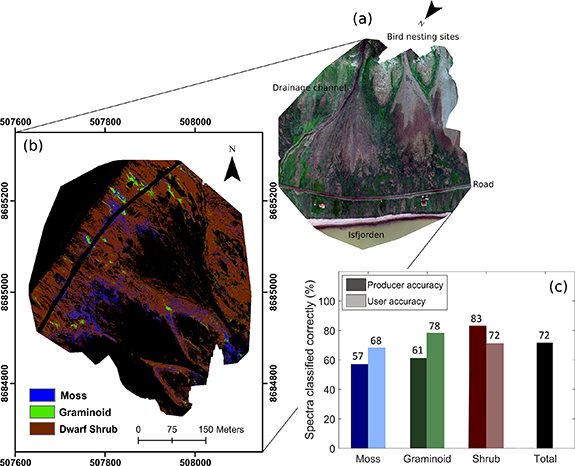
Figure 7. (a) Annotated RGB image of the Birdcliff site. The image has been rotated to represent decreasing elevation from top to bottom. (b) Map of moss, graminoid and dwarf shrub distribution across the Birdcliff site. Produced using UAV reflectance spectra and Random Forest Classification. (c) User and producer accuracy of the model applied to the validation dataset.
Download figure:
Standard image High-resolution image3.4. UAV spectral mapping of plant traits
Using the UAV five-band data, average correlations with water and N were significantly lower (p< 0.001) than when using the downscaled hyperspectral data (figure 8). Plant water trait correlations decreased from r2 = 0.68 to r2 = 0.50 and N accuracies decreased from r2 = 0.76 to r2 = 0.50. The exception was P, where the average correlations between the UAV spectroscopy and field measurements increased from r2 = 0.45 to r2 = 0.54 compared to the downscaled hyperspectral data. Scaling up the most robust models, there was a clear plant water and nutrient gradient across the site. Plant water and nutrient values were generally highest at the top of the nutrient and elevation gradient and declined downslope. Nutrient concentrations also appeared to follow drainage channels across the site and were tightly correlated to each other.
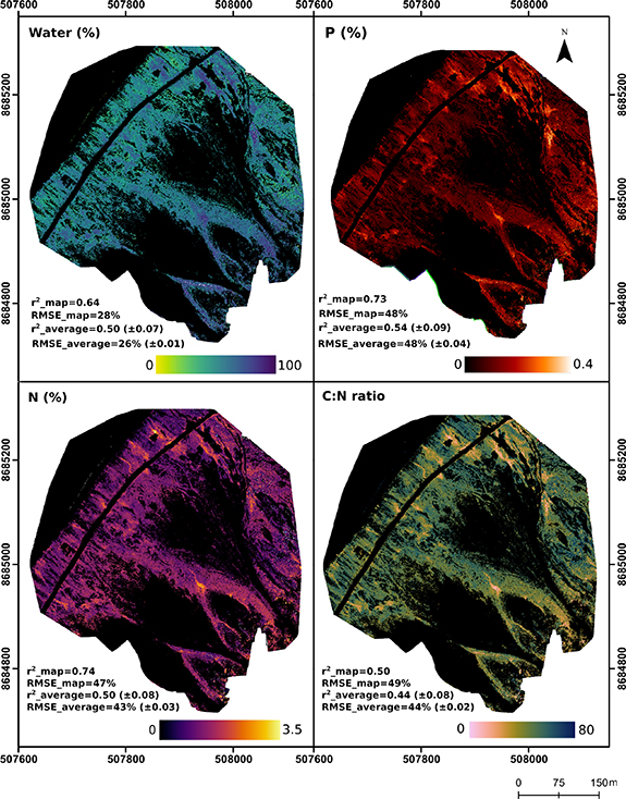
Figure 8. Maps of plant water, nitrogen, phosphorus and C:N ratios across the Birdcliff site. The maps were produced using UAV spectra and partial least squares regression PLSR). r2_map and RMSE_map represent the PLSR model that was chosen to scale up the results of the calibration/validation dataset. r2_average and RMSE_average are the average of 1000 PLSR runs.
Download figure:
Standard image High-resolution image3.5. Sentinel-2A spectral mapping of plant water content
Scaling from the UAV to the satellite level, calibrating a Sentinel-specific PLSR model on the UAV plant water map values (figure 9(a)) and applying the UAV plant water model directly to the Sentinel imagery (figure 9(b)) produced similar patterns but a very different magnitude of result. The maps were correlated with each other at r = 0.86, with a y-intercept of 41%. For method A, plant water content values ranged between 30% and 80%, while method B overestimated water content, with values ranging from 80% upwards.

Figure 9. Two methods of mapping vegetation water content (%) around Longyearbyen, Svalbard using the UAV-generated plant water map in figure 8 and Sentinel-2A imagery. Method (a): calibrating a Sentinel-specific PLSR model (ten bands) on the UAV plant water map values and applying it across the imagery. Method (b): applying the UAV plant water PLSR model (five bands) to the closest corresponding Sentinel-2 bands. The cloud-free Sentinel-2 image was taken on 30 July 2018.
Download figure:
Standard image High-resolution image
4. Discussion
Our results show that UAV multispectral data can be used to map fine-scale vegetation cover (moss, graminoids and dwarf shrubs) across the High Arctic and monitor changes in plant water and nutrient traits. Using field spectroscopy data, we were able to distinguish eight common tundra species at 74% accuracy, suggesting good prospects for near-future vegetation mapping at the species level with the increasing commercialisation of UAV–hyperspectral systems and next generation of hyperspectral satellites (CHIME, EnMAP, HISUI, HypXIM, HyspIRI, PRISMA etc [94–99]). Although only CHIME, EnMAP and PRISMA cover the high latitudes (extending to 84° N, 80° N and 70° N respectively), hyperspectral technology in this area is expanding.
Mosses in particular displayed a unique spectral signature and distinct spectral separability within tundra vegetation. Average moss reflectance across the NIR and SWIR was lower than for graminoids and shrubs, reflecting their lack of vascular system and high water content. All three families/genera of moss, Aulacomnium, Polytrichaceae and Racomitrium, displayed high prediction accuracies in the Random Forest analysis (85, 80% and 80% respectively), which is promising for the automatic detection of moss taxa in future hyperspectral studies. In northern environments, mosses can dominate aboveground primary productivity and have been shown to display a wide range of traits and life history strategies [100–103]. Yet, due to the difficulty of identifying species, mosses are often ignored by ecologists in favour of vascular plants, or conglomerated into groups that may or may not be meaningful [104]. Thus, the ability to distinguish moss taxa at broad scales would facilitate research focusing on this significant but understudied plant group.
Graminoids showed similar spectral separability with a 73% and 80% prediction accuracy for Alopecurus ovatus and Luzula, respectively. Salix polaris also demonstrated a high prediction accuracy of 80%, whereas some spectral confusion was created between the two evergreen dwarf shrubs, Cassiope and Dryas, likely due to Cassiope's woody vertical structure that created high variation in its spectral signature (figure 3). Developing spectroscopic techniques to improve the identification of dwarf shrub species would be useful at broad scales as, along with snow depth, the litter quality of Cassiope, Dryas and Salix has been linked to differences in soil organic matter and respiration rates [105]. Cassiope, Dryas and Salix also display contrasting evergreen and deciduous strategies, which govern different relationships between soil nutrient availability, photosynthesis and growth rates [106]. Overall, these results are highly encouraging with respect to the spectral separability of tundra vegetation and application of fine-scale remote sensing in the Arctic.
At the trait level, we found that four plant traits (water, N, P and C:N values) could be estimated with varying accuracy using field spectroscopy. Plant water and N concentrations were strongly correlated with the full range spectra and showed good agreement with previous PLSR studies at the leaf and canopy scale (e.g. [91, 107, 108]). The estimation of P was slightly lower than previous studies (e.g. [91, 106, 109, 110]), although the PLSR models still captured a substantial amount of variation across the data. Unlike water and N, P has no direct expression across the 400–2500 nm spectrum. Predictions result from correlations with other traits, especially nitrogen, attributed to the stoichiometric link between N and P—a link which has been used to map leaf P across large areas of the tropics and identify crop-level P deficiencies ([111–113]). In contrast to forest or agricultural studies however, N:P ratios may differ more widely among our samples, through different plant groups having fundamentally different N:P ratios ([114]) and high nutrient deposition from bird colonies leading to uneven N:P soil ratios.
When downscaling the hyperspectral data, estimations of plant water content showed a corresponding decrease in accuracy with the number of reduced spectral bands. The nutrient traits were less sensitive to reduced SWIR information, reflecting that water is expressed in a wide range of spectral bands across the VNIR–SWIR spectrum [53], whereas N is a major component of chlorophyll with strong expression in blue and green VIS bandwidths (430–660 nm [53, 115]). P displayed similar spectral weightings to N although, when downscaled to the five MicaSense bands, P values were highly sensitive to a reduction in VNIR information (as similarly found by [110, 116]). In contrast, N showed no significant reduction in accuracy across the downscaled analyses, further suggesting that, in Arctic environments, estimations of P arise from collinearities with traits other than N. We have confidence that the models are detecting trait variation, rather than species-level differences, given the observed spectral weightings and high intraspecific trait variation within Arctic plant functional groups (see table S1 and [117]).
Using the multispectral UAV data, we were able to map moss, graminoids and dwarf shrubs at 72% accuracy. Forbs were not included in the model, as the vegetation cover of any individual forb species was not extensive enough to sample sufficiently. In future studies, it would be useful to test whether forbs can be spectrally distinguished from graminoids (as found by [80] using multispectral satellite imagery, LiDAR and phenology), or whether their similar functionality render forbs and graminoids too related to be differentiated by spectra alone.
Across the Birdcliff site, modelled vegetation distribution was dominated by shrub cover. High nutrient input from nesting colonies generally leads to the formation of moss tundra below bird cliffs on Svalbard [118, 119], but along warmer coastlines, such as Bjørndalen, vascular plants have been found to proliferate [120]. Although moss only constituted 10% of the vegetation cover across the site, the ability to separate moss-dominated pixels from shrubs and graminoids is a key strength of high-resolution mapping over satellite-scale analyses. Regular monitoring of moss communities can act as an early warning system for climatic shifts and associated biotic and abiotic effects in polar environments [121–123]. However, it is important to remember that this study represented a snapshot in time, where moisture conditions, illumination conditions and phenological phase were unique. Time-series data is required to investigate whether moss and other vegetation types can be distinguished with the same accuracy at different phenological stages and under varying abiotic conditions [124, 125].
Using the UAV imagery, we were unable to distinguish vegetation at the species level. This is despite the downscaled hyperspectral data displaying species level accuracy of 64%. We attribute this loss in accuracy to two main reasons. Firstly, UAV imagery suffers from quality issues to a greater extent than field-measured spectra. These include bidirectional reflectance distribution function effects, variability in illumination conditions during a flight, poor radiometric calibration and spectral mixing, even at high resolutions [126, 127]. These effects are even more pronounced in the Arctic due to low sun angle, variable cloud cover and heterogeneous tundra. While the UAV imagery shows a correlation with the field-collected spectra (figure S2), there is substantial variation in the agreement, with the UAV spectra likely exhibiting more statistical error. This may explain why the highest accuracies in our analyses were achieved by averaging spectra from a square of nine pixels (18 × 18 cm) rather than extracting single pixels, due to the increased signal-to-noise ratio of the averaged spectra.
Secondly, accurate geolocation of the ground-truthed vegetation points can be challenging. Across the Arctic, species distribution is extremely heterogeneous and ground-truthing points may only define species presence within a radius of <20 cm. Although RMS errors for the orthomosaics were low (<0.14 m), this could still have resulted in an offset between the ground-truthed vegetation points and the imagery, leading to some inaccuracies in the calibration and validation points. Thus, in environments with high spatial heterogeneity, extremely precise georeferencing equipment is required to accurately calibrate and validate the information collected from UAVs. We recommend covering vegetation around ground-truthing points to create an exclusion zone, or similar methods to reduce the spectral effect of nearby species. In addition, when dealing with mixed plant communities, novel spectral methods are required to capture the co-occurrence of plant types. Rather than discrete vegetation categories, a more flexible model may be required, that removes individual classifications and instead places a vegetation pixel on a continuum of values between moss, graminoid or shrub.
At the landscape level, plant trait distributions displayed a steep water and fertility gradient from the bird cliff colony to the sea, mediated by geomorphology. Plant water content was highest directly underneath the bird colonies and at the confluence of drainage channels. N, P and C:N values indicated well-fertilised vegetation under nesting sites and reflected the transport of nutrients downslope through a network of drainage channels. For example, plant water and nutrient levels were extremely high in the depositional area below the snowmelt channel (figure 7), demonstrating the role that run-off processes play in distributing marine-derived organic matter across the otherwise nutrient-limited tundra. While graminoids constituted just 4% of the vegetation cover across the mapped area, they were mostly found in moist, fertile areas, reflecting their fast growth rates and ability to take swift advantage of available nutrients [128]. This suggests that increased mineralization rates under a warming climate may preferentially benefit graminoid species (as found by [129–131]).
Adding to our confidence that the models were predicting traits explicitly, rather than through correlations with plant type, vegetation cover or productivity, multispectral methods of plant trait retrieval showed a clear independence from NDVI-based predictions (figure S3). With the exception of C:N ratios, neither measured nor predicted trait values were significantly correlated with NDVI, demonstrating the value of a multispectral mapping approach and the lack of physical basis for using NDVI to predict plant traits in the Arctic.
Scaling from the UAV to satellite level, we found different methods of upscaling had a large effect on the magnitude of results, but little influence on the spatial pattern of trait values. Although we do not present either map in figure 9 as accurate, or have the data to validate either map, we found that method A (calibrating Sentinel imagery on UAV-derived plant water values) produced more varying and realistic trait values than method B (applying a UAV plant water model to Sentinel imagery). The higher variation in trait values using method A is probably due to the greater number of spectral bands used in the analysis. In method A, all the relevant Sentinel bands were included as predictors (ten in total), whereas in method B, only the five Sentinel bands that best matched the spectral bands of the MicaSense camera could be used by the UAV plant water model. The overestimation of trait values in method B demonstrates the difference in reflectance captured by UAVs and satellites (see figure S4). Cross-sensor differences arise from atmospheric effects (e.g. haze), differences in viewing and illumination angles, sensor specifications (e.g. bandwidths), and non-linear spectral mixing at different spatial resolutions [32, 127, 132, 133], meaning predictive models generated from one type of imagery cannot be directly applied to another with the same accuracy.
To upscale from UAV to satellite imagery therefore, we recommend creating satellite-specific models calibrated on UAV maps (e.g. method A). Similar methods have been used for a variety of ecological-mapping tasks, such as tree species classification, percentage vegetation cover, agricultural assessments, habitat mapping and fire severity quantification [66, 90, 134–139]. To the best of our knowledge however, this is the first time that upscaling from UAV to satellite imagery has been used to quantify plant traits. With greater UAV coverage across the landscape and more accurate UAV-models (r2 > 0.9), using UAV information to calibrate satellite-based models may provide a valuable method for expanding spatially limited plot studies across the Arctic.
5. Conclusion
Using field spectroscopy, we showed that eight common Arctic plants can be distinguished at the species level at 74% accuracy. These results are relevant for UAV-hyperspectral systems, the first Arctic passenger aircraft equipped with hyperspectral instruments [140] and upcoming hyperspectral satellites, which should be able to use similar methods explored here to advance these results and expand them over a wider geographical area.
Using UAV multispectral information, we have shown that High Arctic moss-, graminoid- and dwarf shrub-dominated vegetation can be mapped at high resolution (<10 cm) with 72% accuracy, alongside corresponding water, nitrogen, phosphorus and C:N values. We present two methods of upscaling these results using Sentinel-2A imagery. The majority of Arctic tundra regions remain under-investigated and difficult to access for scientific research. We must continue to develop methods to expand spatially-limited plot studies, which inherently cannot capture landscape-level vegetation patterns or functional trait variation, in order to monitor environmental change across the Arctic and understand the mechanisms driving large-scale climate-vegetation feedbacks.
Acknowledgments
We thank Plant Functional Trait Course 4 for the funding and logistics that enabled the data collection. We thank the course instructors and course participants for their help and collaboration during the data collection and processing. We also thank Christine Schirmer and the students at the University of Arizona for their assistance with the chemical analyses.
Data availability statement
The data that support the findings of this study are openly available at the following URL/DOI: https://osf.io/smbqh/.
Funding
The data collection was funded by a Norwegian Research Council INTPART Grant (Project Number: 274831), two SIU-foundation projects (UTF-2013/10074 and HNP-2015/10037) and a Research Council of Norway Arctic Field Grant (Project Number: 282611, RiS: 10935). E R T is funded by NERC DTP award (NE/L002612/1). Y M is supported by the Jackson Foundation. M M-F was supported by a NERC IRF (NE/L011859/1).