

Abstract
Rising emissions of anthropogenic greenhouse gases (GHG) have led to tropospheric warming and stratospheric cooling over recent decades. As a thermodynamic consequence, the troposphere has expanded and the rise of the tropopause, the boundary between the troposphere and stratosphere, has been suggested as one of the most robust fingerprints of anthropogenic climate change. Conversely, at altitudes above ∼55 km (in the mesosphere and thermosphere) observational and modeling evidence indicates a downward shift of the height of pressure levels or decreasing density at fixed altitudes. The layer in between, the stratosphere, has not been studied extensively with respect to changes of its global structure. Here we show that this atmospheric layer has contracted substantially over the last decades, and that the main driver for this are increasing concentrations of GHG. Using data from coupled chemistry-climate models we show that this trend will continue and the mean climatological thickness of the stratosphere will decrease by 1.3 km following representative concentration pathway 6.0 by 2080. We also demonstrate that the stratospheric contraction is not only a response to cooling, as changes in both tropopause and stratopause pressure contribute. Moreover, its short emergence time (less than 15 years) makes it a novel and independent indicator of GHG induced climate change.
Export citation and abstract BibTeX RIS

Original content from this work may be used under the terms of the Creative Commons Attribution 4.0 license. Any further distribution of this work must maintain attribution to the author(s) and the title of the work, journal citation and DOI.
1. Introduction
Over the last decades increasing concentrations of greenhouse gases (GHG) have substantially affected the Earth's radiative balance, leading to pronounced warming of the troposphere and cooling of the stratosphere (Stocker et al 2013). The thermal expansion of the troposphere and the associated increase in tropopause height have been proposed as robust fingerprints of anthropogenic climate change based on multiple observational and model evidence (Santer et al 2003, Seidel and Randel 2006, Lorenz and DeWeaver 2007, Heus et al 2009). At the same time, in the mesosphere and above, a downward shift of the height of pressure levels or decreasing density at fixed altitudes were documented (Lubken et al 2013, Jacobi 2014, Stober et al 2014, Emmert 2015, Lima et al 2015, Peters and Entzian 2015, Solomon et al 2018). While a rich body of literature has documented the expansion of the troposphere (Añel et al 2006, Gettelman et al 2009, Eyring et al 2010, Kim et al 2013, Vallis et al 2015) much less attention has been given to the changing global structure of the stratosphere. The latter is not only the home of the ozone layer, but also a radiatively important region in terms of other GHG (e.g. N2O, CO2, H2O, CH4) and dynamically coupled with the troposphere (Baldwin and Dunkerton 2001, Gerber 2012, Kidston et al 2015). Therefore, the structure of the stratosphere is crucial to correctly comprehend atmospheric dynamics and tracer transport, particularly when this atmospheric layer should be disturbed through possible sulfate geoengineering experiments where the altitude of injection plays a key role (Tilmes et al 2018, Visioni et al 2021). Compared to the troposphere, where considerable multi-instrumental global observational data are available, homogenous global observations spanning the full stratospheric vertical extent and the stratopause region (located around an altitude of 50 km) are sparse and/or of limited temporal duration (Clancy and Rusch 1990, Russell et al 1993, Dunkerton et al 1998, Remsberg et al 2008, Schwartz et al 2008, Remsberg 2009, Hauchecorne et al 2019). As the stratosphere has substantially cooled in the last several decades (Randel et al 2016, Steiner et al 2020), including a near global cooling in the stratopause region (Remsberg 2019), one might expect accompanying thickness changes (of the stratosphere) from simple thermodynamic considerations (Akmaev, 2012, Rishbeth 1990, Akmaev 2002, Akmaev et al 2006, Yuan et al 2019). Such, decreasing stratospheric thickness trend (contraction) has so far, however, been reported only locally and over a short observational time span (Ramesh and Sridharan 2018). Here we use data from state-of-the-art coupled chemistry-climate models (CCMs) to address, whether stratospheric contraction occurs and will occur on global scale, and if so, to which extent past contraction has been driven by changes in GHG or ozone depletion (Akmaev, 2012, Rieder et al 2014), given that both are main drivers of stratospheric temperature change.
2. Data and methods
2.1. Data
We use output of an ensemble of chemistry-climate models, which all contributed to the Chemistry Climate Model Initiative (CCMI) (Morgenstern et al 2017). From the set of CCMI scenarios we use an all forcing scenario as baseline, and two sensitivity experiments, one with fixed GHG, the other one with fixed ozone depleting substances (ODS). Throughout the manuscript we refer to these as AllForcings, FixedGHG and FixedODS and within the framework of CCMI these experiments are referred to as REF-C2, SEN-C2fGHG and SEN-C2fODS, respectively. The AllForcings simulations follow the A1 scenario for ozone-depleting substances (WMO 2011) and the RCP 6.0 scenario for other GHG, tropospheric ozone precursors, and aerosol precursor emissions (Meinshausen et al 2011). Anthropogenic emissions are based on MACCity (Granier et al 2011) until 2000, followed by RCP 6.0 emissions. To stabilize the radiative forcing of the RCP 6.0 scenario at 6 W m−2 after 2100, an emission reduction of about 50% below baseline is applied after 2080. This way, for example CO2 stabilizes at 752 ppm in the 22nd century, which rests on the assumption that stringent post-2100 emission reductions are feasible (Meinshausen et al 2011). In these simulations some models (MRI, NIWA-UKCA, HadGEM, GFDL, CESM, CHASER, and WACCM) have coupled an interactive ocean and sea ice module for atmosphere-ocean interactions, while other models impose sea surface temperatures and sea ice concentrations, using a variety of different climate model data sets for this purpose (e.g. HadISST1 or HadGEM2 data; for details see table S1 in Morgenstern et al 2017). The FixedGHG and FixedODS experiments are sensitivity simulations of the same base configuration as the AllForcings simulations but with GHG or ODS fixed at their 1960 level, and sea surface and sea ice conditions prescribed as the 1955–1964 average (where these conditions are imposed). Note, not all CCMI models which have delivered AllForcings integrations have also delivered the FixedGHG and FixedODS sensitivity experiments (see supplemental table S1 (available online at stacks.iop.org/ERL/16/064038/mmedia)).
Along with the CCM model output we analyze three widely used reanalyses. The presented tropopause height analysis for 1980–2018 is based on three reanalysis products: ERA-5 (Hersbach et al 2020, C3S 2017), JRA-55 (Kobayashi et al 2015) and MERRA2 (Gelaro et al 2017). The analysis of geopotential height trends for 1960–2018 is based on JRA-55. For comparison of model results with reanalyses we focus on the 1980–2018 time period. For the analysis of the AllForcings, FixedODS and FixedGHG experiments we examine the long-term period 1960–2080, as well as the two subperiods 1960–1999 and 2000–2080, with the year 2000 chosen as the breakpoint given the reversal of the ODS trend around the turn of the century.
2.2. Metrics of tropopause and stratopause height
The tropopause and stratopause heights have been identified (in geopotential coordinates) for each individual model participating in CCMI, for the AllForcings, FixedODS and FixedGHG experiments (Eyring et al 2013). If multiple ensemble members have been available for an individual model, only the first ensemble member has been used in our study (to ensure equal weighting of participating models). We have interpolated the data into a common vertical resolution of 100 m. The tropopause height has been determined as the first lapse rate tropopause using the WMO definition (WMO 1957): the tropopause is defined as the lowest level at which the lapse rate decreases to 2 °C km−1 or less, provided that the average lapse rate between this level and all higher levels within 2 km does not exceed 2 °C km−1. We use geopotential height as a proxy for geometric altitude as in a geometric coordinate system the net tropopause trend consists of the trend in geopotential height of pressure levels and the trend relative to the pressure levels. The stratopause height has been calculated as the level of maximum temperature between 40 and 65 km altitude. Stratospheric thickness has been calculated as the difference between the tropopause height and stratopause height. Ensemble mean values are calculated as arithmetic mean across the available model integrations per experiment. Trends for all variables considered have been estimated (from yearly time series calculated from monthly means given by the original data) by the Theil–Sen estimator and their significance at the 95%-level has been determined using the Mann–Kendall test. If outliers are displayed (such as in figure 2) they are defined as exceeding 1.5 times the inter-quartile range. The emergence time of the stratospheric thickness trend was calculated as the minimum length of the stratospheric thickness time series where a statistically significant trend was detected.
2.3. Determining the contribution of changes in temperature, tropopause pressure and stratopause pressure to changes in stratospheric thickness
The contribution of changes in temperature and tropopause and stratopause height to the net stratospheric contraction is evaluated based on the hypsometric equation, which in the form below yields an approximation for the stratospheric thickness at a leading order:
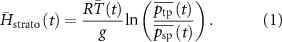
Here,  is the global mean stratospheric thickness estimate,
  is the global mean stratospheric temperature and
  are the global mean tropopause and stratopause pressures, respectively. g denotes the acceleration of gravity (9.806 m s−2) and R is the dry air gas constant (287.058 J kg−1 K−1).
The relative contributions to the global mean stratospheric thickness change are derived from the global mean stratospheric temperature and pressure of the pauses by differentiating equation (1) to obtain:
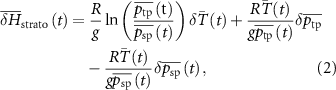
where  is a simple linear operator chosen as a rate of change per year (
 ) in our case. The individual contributions of changes in temperature, tropopause pressure and stratopause pressure to the change in stratospheric thickness are defined as an average contribution from corresponding terms in equation (2) over a time period in consideration. The hypsometric estimate approximates the evolution of stratospheric thickness very accurately (see figure S1) justifying the analysis of stratospheric contraction on a global scale.
3. Results
3.1. Stratospheric contraction
For the height evolution of the stratospheric lower bound, the tropopause, CCMs are in excellent agreement with observations. We illustrate this for the recent past (1980–2018) in figure 1(a) by contrasting rising trends of the annual mean tropopause height simulated by the CCMI models with those of three widely used reanalyses (MERRA-2, ERA-5, JRA55; see methods). The tropopause height in the reanalyses fall well within the range simulated by CCMs. Looking into the future, we here confine ourselves to the year 2080, as GHG concentrations change non-monotonically after 2080 for the AllForcings scenario. Over the entire 1960–2080 period a monotonic increase in the tropopause height is clearly seen (figure 1(b)). From the tropopause we now examine higher levels. Unfortunately, a clean analysis comparable to the troposphere is not feasible for the stratosphere as at these levels reanalysis data cannot be considered a pure observational proxy. However, stratospheric cooling in recent decades is well documented, and the CCMI models are in good agreement with the temperature measurements from satellites throughout the stratosphere (Randel et al 2017, Maycock et al 2018), lending confidence that CCMs can also faithfully simulate other aspects of stratospheric changes. Notably CCMs indicate a robust decline in the stratopause height (figure 1(c)), which is projected to continue over the 21st century (figure 1(d)). Bounded between the tropopause and stratopause, and due to their respective rising and falling, the stratosphere therefore has been experiencing a global mean net contraction (figure 1(e)). That this contraction is underway and is projected to continue into the late 21st century (figure 1(f)) is the key finding of our paper, a simple fact that, to the best of our knowledge, has not been reported to date. In quantitative terms, the CCMI AllForcings simulations indicate that the mean climatological thickness of the stratosphere decreases by 1.3 km until 2080 (representing a 3.7% change from the 1980–2018 mean).

Figure 1. Anomalies (from the 1980–2018 reference period) of the tropopause height (a), (b), stratopause height (c), (d) and the stratosphere thickness (e), (f) for 1980–2018 (left) and 1960–2080 (right). The solid black line illustrates the mean of all included CCMI models and the red line represents the mean of the included reanalyses. All model simulations are for the AllForcings experiment. The shaded areas show the spread (min to max) of the CCMI models.
Download figure:
Standard image High-resolution image3.2. Anthropogenic forcing
The two likely anthropogenic forcings underlying the contraction illustrated above are GHG and ODS, given that there is now a larger body of literature demonstrating their roles in recent and future trends in stratospheric temperature, circulation and composition (i.e. ozone layer depletion and recovery). In recent years, it has been shown that a number of climate system trends that have been previously assumed to be predominantly GHG-induced are, to a significant extent, driven by ODS (Polvani et al 2020) or, indirectly, through changes in ozone caused by ODS (Polvani et al 2011, Rieder et al 2014, Banerjee et al 2020). However, as far as stratospheric contraction is concerned, figures 1(b), (d) and (f) shows that all trends continue monotonically throughout the 20th and 21st century: this suggests that GHG dominate over ODS, because GHG concentrations are projected to monotonically increase, whereas ODS concentrations peaked in the late 20th century and will be decreasing in coming decades as a consequence of the Montreal Protocol (WMO 2018).
To confirm this, we have analyzed the CCMI simulations with one of these forcings held fixed (FixedGHG or FixedODS, see methods) along with the AllForcings simulations. In figure 2 we show trends in tropopause height (top row), stratopause height (middle row) and stratospheric thickness (bottom row) in these three sets of simulations over three different time periods: 1960–2080 (left column), 1960–1999 (middle column) and 2000–2080 (right column). The 1960–1999 period is of particular interest given the monotonic increase in both GHG and ODS concentrations during those decades, and the availability of observational evidence for tropopause height from atmospheric reanalyses. Figure 2(a) shows that both increasing GHG and ODS result in increasing tropopause height. In the 20th century (panel b) the change resulting from increasing GHG is about twice the change attributable to ODS. However, in the 21st century (panel c), the bulk of tropopause trends is due to GHG, with ODS contributing only a small and opposite trend as the ozone layer recovers. Consistent with this finding, the trend in the FixedODS simulations is larger than that in AllForcings. Turning next to stratopause height trends, they are generally negative (figures 2(d)–(f)). In the 21st century, FixedGHG simulations show negligible stratopause height trends, while FixedODS simulations show substantial negative stratopause height trends (panel f), which are of the same magnitude as in AllForcings.

Figure 2. CCMI model trends (m decade−1) in tropopause height (top row), stratopause height (middle row) and the stratospheric thickness (bottom row) for the 1960–2080 (left hand column), 1960–1999 (middle column) and 2000–2080 (right hand column) period. The open circles mark the outliers. The numbers on the x axis denote the number of models included (i.e. models with significant trends).
Download figure:
Standard image High-resolution imageTaken together the changes in tropopause and stratopause height result in a pronounced decrease in stratospheric thickness, which we can largely attribute to changes in GHG (figures 2(g)–(i)). In connection to this, the net stratospheric contraction is characterized by a short trend emergence time (less than 15 years, see figure S2). We have verified that this contraction is largely independent of temporal or regional subsampling (i.e. global mean data as well as for latitudinal bands and seasons). The only exception are Southern polar latitudes over the 1960–1999 period, when ODS contribute to stratospheric contraction via radiative cooling accompanying ozone depletion by an amount comparable to that of GHG (figure S3); this reverses in the 21st century, as the ozone layer recovers (figure S4).
3.3. Role of the stratospheric cooling
We next address the questions of whether stratospheric contraction is a mere consequence of stratospheric cooling, or whether other (possibly dynamical) mechanisms are at play. For this, we separate the stratospheric thickness changes (by differentiating the hypsometric equation, see methods) into the changes in stratospheric temperature and changes in tropopause or stratopause pressure (table 1). This separation shows that while the change in temperature is the dominant contributor, changes in tropopause and stratopause pressure also add significantly to the net contraction of the stratosphere. The contribution of stratopause pressure to the contraction of the stratosphere is of particular note, as it reverses from negative to positive sign between 1960–1999 and 2000–2080. Positive values indicate that the changes of a particular parameter enhance the contraction, and negative values reduce it. The reversal from negative to positive in case of the stratopause pressure is attributable to the effects of a changing burden in ODS on ozone, as ODS peak around the year 2000 (WMO 2018). For 1960–2000 the stratopause pressure trend is of opposite sign than the trends of the other two forcings, thereby reducing the total trend. Values of the contributions for the FixedGHG and FixedODS simulations are shown in the supplemental table 2. We note in passing that the contributions in the FixedGHG simulations are very large because the stratospheric thickness trends in these simulations are near zero (see figure 2) and even a small forcing may contribute to a change proportionally larger than the resulting contraction.
Table 1. Contributions to the stratospheric contraction. Contribution of changes in stratospheric temperature, tropopause pressure, and stratopause pressure to the change in stratospheric thickness (derived from the hypsometric equation) expressed as % over the corresponding time period for the AllForcings simulation.
| Contribution by changes in | 1960–1999 | 2000–2080 |
|---|---|---|
| Stratospheric temperature | 83.7% | 52.7% |
| Tropopause pressure | 36.9% | 25.9% |
| Stratopause pressure | −20.6% | 21.4% |
3.4. Vertical structure
Finally, we show how the stratospheric contraction affects the vertical structure of the atmosphere. Figure 3 illustrates, how the tropospheric expansion marked by positive geopotential height trends is gradually weakened above the tropopause by the overlying stratospheric contraction and then overcome in the mid stratosphere, leading to negative geopotential height trends at upper levels. The solid lines in figure 3 show the mean pauses calculated from the ensemble comprising the respective model and simulation pairs. For example, the solid lines in 3a represent the mean tropopause and stratopause calculated as an average of the pauses detected in the models providing the AllForcings simulation. The mean pauses are calculated separately for the AllForcings, FixedODS and FixedGHG simulations: this explains the small differences in panels 3a, 3b and 3c. The FixedGHG simulations demonstrate that ODS significantly affect the structure of the stratosphere mainly in the tropics (in the annual mean), where they cause a nearly uniform shift of the pressure levels, resulting in a net null effect on stratospheric thickness (figures 3(c) and (g)). Figure 3 also shows that over the 1960–1999 period, reanalysis data (figure 3(d)) and model simulations with AllForcings (figure 3(a)) or FixedODS (figure 3(b)) agree well regarding the latitudinal distribution of geopotential height trends. The magnitude and latitudinal extent of the upward shift in the upper troposphere and lower stratosphere, however, appears to be slightly overestimated by the models, with the transition from an upward to a downward shift occurring at lower altitude in reanalysis data than in CCMs. For the 2000–2080 period we find a significant vertical shift also in the polar regions (figures 3(e)–(f)). This trend is stronger in the FixedODS simulations (figure 3(f)) than when the transient evolution of ODS (figure 3(e)) is prescribed. The most important feature of figure 3, however, is the indication of an ubiquitous stratospheric contraction over the 21st century, throughout all latitudes, and this being caused primarily by increasing GHG.

Figure 3. Geopotential height trends (m decade−1) for the CCMI models and the JRA-55 reanalysis. The first three columns from the left show the multimodel mean trends for the AllForcings, FixedODS and FixedGHG experiments. The white areas represent statistically insignificant trends. In all panels, the black line below 100 hPa denotes the mean tropopause, and the line around 1 hPa the mean stratopause.
Download figure:
Standard image High-resolution image
4. Summary and conclusions
In summary, we have presented evidence for a substantial contraction of the stratosphere in recent decades. As estimated from an ensemble of CCM simulations, the stratospheric extent has declined by 0.4 km between 1980 and 2018 and models project a net contraction of 1.3 km by the year 2080, corresponding to a 3.7% decline compared to the 1980–2018 mean stratospheric thickness. This negative trend is monotonic with short emergence time, as the contraction is driven almost entirely by GHG. The robustness of this feature is unlikely to be affected by potential trends in solar forcing, which have an opposite thermal effect in this atmospheric region compared to GHG (Rind et al 2008). Our results indicate that the widely recognized cooling of the stratosphere while important, is not the sole driver of the reduced stratospheric extent, with complex radiative and chemical feedbacks likely at play. As model projections for the 21st century show that stratospheric contraction will continue if anthropogenic GHG emission trajectories are not reversed, a detailed understanding and quantification will be increasingly important, as it will entail decreasing density at high altitudes. Eichinger and Sacha (2020) have shown that assuming a constant scale height in the stratosphere can lead to diagnostic misinterpretations of dynamical trends in climate model projections and Zhou et al (2020) have recently analyzed the impact of its variations on the period of the QBO. The contraction may also contribute to changes in stratospheric dynamics or in radiative transfer in the stratosphere (by influencing scale-heights of the absorbers/emitters), but these impacts are yet to be determined and quantified. Moreover, it may affect satellite trajectories, orbital life-times, and retrievals (Schroder et al 2007), and, via indirect influence on ionospheric electron density, the propagation of radio waves, and eventually the overall performance of the Global Positioning System (GPS) and other space-based navigational systems (Lastovicka et al 2006).
Acknowledgments
We acknowledge the modeling groups for making their simulations available for this analysis, the joint WCRP SPARC/IGAC Chemistry-Climate Model Initiative (CCMI) for organizing and coordinating the model data analysis activity, and the British Atmospheric Data Centre (BADC) for collecting and archiving the CCMI model output. We thank Daniel Marsh, Douglas Kinnison, Simone Tilmes from the National Center for Atmospheric Research in Boulder for providing corrected WACCM CCMI Geopotential Height data. The authors thank ECMWF, NCAR and JMA for provision of individual reanalyses data sets via agency gateways. We thank D Burianova, T Labudova, K Voldrich, R Zajicek from the Department of Atmospheric Physics of Charles University in Prague for assistance. PP and PS were supported by GA CR under Grant No. 18-01625S. PP and RE are supported by GA CR under Grant Nos. 21-20293J and 21-03295S. PS is supported through the project CZ.02.2.69/0.0/0.0/19_074/0016231 (International mobility of researchers at Charles University (MSCA-IF III)) for the research stay at BOKU Vienna and at earlier stages of the manuscript by a postdoctoral grant of Xunta de Galicia ED481B 2018/103. RE and PS acknowledge support from the BTHA under Grant No. BTHA-MOB-2020-2. LMP is funded by a grant from the US National Science Foundation to Columbia University. JA was partially supported by a Ramón y Cajal Grant (RYC-2013-14560) and the work was started during the ZEXMOD Project, both funded by the Government of Spain (CGL2015-71575-P). The EPhysLab is supported by the European Regional Development Fund and the Xunta de Galicia (ED431C 2017/64-GRC). RE is supported by the Helmholtz Association under Grant No. VH-NG-1014 (Helmholtz-Hochschul-Nachwuchsforschergruppe MACClim). AK and CJ acknowledge support from Deutsche Forschungsgemeinschaft under Grant No. JA836/43-1 (VACILT).
Data availability statement
The reanalysis datasets used in this study can be downloaded from their respective provider webservers at: ERA5 reanalysis data are available from the Copernicus Climate Data Store (https://cds.climate.copernicus.eu/), JRA-55 series are provided from the Japanese 55 year Reanalysis project carried out by the Japan Meteorological Agency (https://jra.kishou.go.jp/JRA-55) and MERRA-2 reanalysis data are available from the Global Modeling and Assimilation Office at NASA GSF (https://gmao.gsfc.nasa.gov/reanalysis/MERRA-2/). Model output from CCMI can be accessed through the British Atmospheric Data Center (BADC) archive (http://data.ceda.acuk/badc) and The WACCM CCMI data are available from NCAR Climate Data Gateway (www.earthsystemgrid.org/search.html?Project=CCMI1).
The data that support the findings of this study are openly available at the following URL/DOI: https://data.ceda.acuk/badc/wcrp-ccmi/data/CCMI-1/output.