

Abstract
Many land-based ecosystems are dependent on groundwater and could be threatened by human groundwater abstraction. One key challenge for the description of associated impacts is the initial localisation of groundwater-dependent ecosystems (GDEs). This usually requires a mixture of extensive site-specific data collection and the use of geospatial datasets and remote sensing techniques. To date, no study has succeeded in identifying different types of GDEs in parallel worldwide. The main objective of this work is to perform a global screening analysis to identify GDE potentials rather than GDE locations. In addition, potential risks to GDEs from groundwater abstraction shall be identified. We defined nine key indicators that capture GDE potentials and associated risks on a global grid of 0.5° spatial resolution. Groundwater-dependent streams, wetlands and vegetation were covered, and a GDE index was formulated incorporating the following three aspects: the extent of groundwater use per GDE type, GDE diversity and GDE presence by land cover. The results show that GDE potentials are widely distributed across the globe, but with different distribution patterns depending on the type of ecosystem. The highest overall potential for GDEs is found in tropical regions, followed by arid and temperate climates. The GDE potentials were validated against regional studies, which showed a trend of increasing matching characteristics towards higher GDE potentials, but also inconsistencies upon closer analysis. Thus, the results can be used as first-order estimates only, which would need to be explored in the context of more site-specific analyses. Identified risks to GDEs from groundwater abstraction are more geographically limited and concentrated in the US and Mexico, the Iberian Peninsula and the Maghreb, as well as Central, South and East Asia. The derived findings on GDEs and associated risks can be useful for prioritising future research and can be integrated into sustainability-related tools such as the water footprint.
Export citation and abstract BibTeX RIS

Original content from this work may be used under the terms of the Creative Commons Attribution 4.0 license. Any further distribution of this work must maintain attribution to the author(s) and the title of the work, journal citation and DOI.
1. Introduction
The preservation of major land ecosystems is fundamental to sustainable development (Chaplin-Kramer et al 2022). Land ecosystems and their associated biodiversity should be protected not only for their intrinsic value (Batavia and Nelson 2017, Sheng et al 2019), but also for their ecosystem services (Mitchell et al 2021), such as supporting global food and water security or climate change mitigation (IPBES 2019).
Many ecosystems on land are supported by groundwater resources and can be considered groundwater-dependent to varying degrees (Pérez Hoyos et al 2016, UNDP 2022). Within this context, Eamus et al (2016) defined three general types of groundwater-dependent ecosystems (GDEs): 1. aquifer and cave ecosystems; 2. ecosystems reliant on the surface expression of groundwater (e.g. base flow rivers and streams, wetlands, springs and estuarine seagrasses); and 3. terrestrial ecosystems reliant on the subsurface presence of groundwater within the rooting depth of vegetation (e.g. phreatophytic ecosystems).
Due to growing human demand for water, GDEs are under increasing threat worldwide, which has already led to water management initiatives (e.g. in Australia, the EU, South Africa and the US) to protect such ecosystems (Rohde et al 2017). Groundwater is the world's largest accessible freshwater resource, making up about 97% of the total liquid freshwater on Earth (Aeschbach-Hertig and Gleeson 2012, Stone et al 2019) and accounting for about 37% of global water consumption (UNDP 2022). Globally, groundwater extractions have already led to falling water tables (Jasechko and Perrone 2021) and even widespread groundwater depletion (Aeschbach-Hertig and Gleeson 2012, de Graaf et al 2017, Bierkens and Wada 2019). This may result in less groundwater discharge to adjacent GDEs, placing them at increased risk of water stress, alteration of ecosystem structure, and reduction of associated ecosystem services (Eamus et al 2006, Murray et al 2006, Eamus et al 2015, Rohde et al 2017). As for the contribution of groundwater to regional runoff, the ecological limits of groundwater pumping have already been exceeded in some regions (de Graaf et al 2019). Therefore, the concept of groundwater sustainability is becoming increasingly important nowadays (Elshall et al 2020, Gleeson et al 2020).
Water consumption and associated impacts on ecosystems can be linked to human production systems. First assessment tools such as the water footprint (ISO 2016) are available to identify potential water-related environmental impacts over products' life cycles. Water footprinting is widely used when making sustainability-based decisions along global supply chains (Berger et al 2021) and provides a wide range of water-related impact assessment methods (Berger and Finkbeiner 2010). However, most methods refer to the environmental impacts of surface water consumption (Hanafiah et al 2011, Tendall et al 2014, Pierrat et al 2023) or do not distinguish between the consumption from different water sources (e.g. Pfister et al 2009, Berger et al 2018, Boulay et al 2018). Methods within this domain focusing exclusively on ecosystem impacts of groundwater abstraction, in contrast, are still in their infancy. Among the ones that do exist, three key methods can be listed: 1. Gleeson et al (2012) developed groundwater footprints (defined as the area required to sustain groundwater use and GDE services) for a number of large aquifers, taking ecosystem requirements for regional streamflow into account; 2. Verones et al (2013a, 2013b) linked groundwater consumption with falling groundwater table depths, losses in wetland areas and biodiversity declines for wetlands of international importance (Verones et al 2013a, 2013b); 3. van Zelm et al (2011) determined potential environmental impacts of groundwater extraction on plant diversity in the Netherlands. All three methods cover only one GDE type and lack continuous coverage across the globe.
One major challenge in describing potential impacts is the worldwide localisation of GDEs (Eamus et al 2015, Kreamer et al 2015). GDEs often represent small-scale features (Kreamer et al 2015) that may span a few meters, but can also reach larger dimensions of several square kilometres (NSW 2022). Depending upon intended level of detail, global mapping of GDEs can thus be associated with considerable effort in terms of data volume and processing and might be affected by inconsistent data availability and quality across regions and between different data types (Eamus and Froend 2006, Kuginis et al 2016, Pérez Hoyos et al 2016, UNDP 2022). The current state of the art in GDE mapping addressing larger regions of regional to continental scale, refers to studies associated with the US (Howard et al 2010, Brown et al 2011, Mathie et al 2011, Gou et al 2015), South Africa (Colvin et al 2002, Münch and Conrad 2007), the Iberian Peninsula (Marques et al 2019, Páscoa et al 2020, Martínez-Santos et al 2021), Central Asia (Liu et al 2021), as well as the Australian continent (Doody et al 2017). These classify GDEs at different resolutions, ranging from watershed level at slightly below 100 km2 (Howard et al 2010, Brown et al 2011) to 25 m spatial resolution (Münch and Conrad 2007, Doody et al 2017, Marques et al 2019). Typically, this involved a mixture of information, including field data, geospatial datasets and means of remote sensing, such as imagery on persisting greenness during a prolonged dry period indicating groundwater-dependent vegetation. Vegetation was the most frequently considered GDE type, followed by wetland, stream, and spring ecosystems. Estuaries with groundwater dependence and marine systems relying on the submarine discharge of groundwater were generally not considered. The same applies to aquifer and cave ecosystems, which provide subsurface habitats for highly specialized organisms of the stygofauna (Eamus et al 2016). S1 presents more detailed overview on the current state of the art within GDE research.
The large amount of site-specific information needed highlights the challenge to globally determine GDEs at fine resolution. To date, no study has achieved this for different GDE types simultaneously. However, we hypothesise that existing geospatial datasets at coarser resolution would allow global screening and spatially distributed basic statements on general occurrence probabilities of GDEs. In conjunction with human pressures such as groundwater pumping, it may then be possible to identify where GDEs may potentially be at risk. This information could be used to prioritise further research and for application in current sustainability tools. The goal of this work is to utilise ready-to-use geospatial datasets to simultaneously screen for potentials of various types of GDEs at global scale. Then, identified potentials are to be validated on the basis of existing studies. Beyond that, GDE probability classes shall be determined and combined with human-induced groundwater stress, resulting in global risk indices for GDEs.
2. Method
2.1. Key data and definition of the grid
The key data source was the global hydrological model WaterGAP2d (Müller Schmied et al 2021). For 2000–2016, we extracted data on average streamflow, actual land evaporation, precipitation, groundwater recharge, groundwater storage, net groundwater abstraction and total water consumption at 0.5° spatial resolution. This resolution also defined our target grid for determining GDEs. Relevant land cells were specified by intersection of the grid with the WWF's global terrestrial ecoregions (Olson et al 2001) excluding Antarctica. This resulted in a total of 69 507 land cells considered. Moreover, the G3M global groundwater model was of importance (Reinecke et al 2019). G3M was previously coupled with WaterGAP2d, and provided averaged data on groundwater table depths, as well as annual groundwater discharge to streams, wetlands, and lakes. Details on WaterGAP2d (Müller Schmied et al 2021) and G3M (Reinecke et al 2019) are summarised in S2.
2.2. Screening for GDE potentials
The top of figure 1 illustrates the screening procedure for deriving GDE potentials. Given the global availability of data, we focused on groundwater-dependent streams, wetlands and vegetation. The first indicator is the stream index (I1), reflecting the contribution of groundwater to average streamflow (Howard et al 2010, Gou et al 2015). The wetland index (I2) instead determines groundwater contribution to wetlands and lakes, considering parallel water inflows from precipitation. The vegetation index (I3) finally addresses groundwater-dependent vegetation. I3 is composed of two equally-weighted sub-indicators. I3.1 represents the potential xylem groundwater fraction of regional vegetation. This draws on a biome-based meta study of xylem water analyses by Evaristo and McDonnel (2017) with additional consideration of datasets for the estimation of groundwater accessibility by plant roots (S3; Ficher et al 2012, Fan et al 2017). I3.2 represents potential inflow dependency (Doody et al 2017). Inflow dependency was determined when land evaporation exceeded precipitation across the year, making alternative water sources such as groundwater likely (Doody et al 2017). It was described through predefined evaporation-to-precipitation thresholds and is most suitable for regions where groundwater is mainly used in dry seasons, such as in temperate and arid climates (Doody et al 2017). For tropical regions, we instead used seasonal groundwater storage ranges based on Doody et al (2017) and related these to regional land evaporation.

Figure 1. Two-part scheme and associated indicators for determining GDE (top box with blue frame) and risk (bottom box with red frame) indices; the indicators I1–I3 represent the potential extent of potential groundwater use for the GDE types streams, wetlands and vegetation; the additional consideration of GDE diversity is represented by the aggregation to an aggregate index (I4); the final GDE index (I6) additionally considers the potential presence of GDEs by the share relevant land covers (I5) and was also the starting point for determining possible risks for GDEs: there, a min–max normalisation and natural breaks classification were carried out to define GDE probability (I7) classes; the final risk indices (I9), on the other hand, were compiled while additionally considering classes of different groundwater stress (I8); the indicators I6–I9 were aggregated to catchment and country scales based on consumption weighted averages; while all indicators reflect a dimensionless value between zero and one, all risk-based indicators (I6–I9) carry an additional descriptive attribution (ranging from very low to very high GDE probability, groundwater stress or risk for GDEs).
Download figure:
Standard image High-resolution imageAfter determining indices for streams, wetlands and vegetation, an aggregate index (I4) was formed using the arithmetic mean in analogy to Howard et al (2010). Then, possible presence of GDEs was further evaluated based on land cover composition (I5; Buchhorn et al 2016). This finally resulted in the GDE index (I6). While indicators I1–I3 express the potential extent of groundwater use per GDE type, their aggregation to I4 led to an index additionally addressing GDE diversity. The GDE index (I6) ultimately incorporates three aspects: the extent of groundwater use per GDE type, GDE diversity and GDE presence by land cover. Full details on the calculations for indicators I1–I6 and associated formulae are found in S4.
2.3. Validation of GDE potentials
GDE potentials were validated against the current state of the art of GDE research at the regional level (S1). The regional studies for comparison were selected according to the accessibility of study outputs and aimed to cover different GDE types and world regions. The following cases were utilised and compared with the most fitting indicators from our work or combinations thereof: 1. groundwater-dependent surface water systems in the US federal state of Oregon (Brown et al 2011); 2. groundwater-dependent vegetation in arid climates on the Iberian Peninsula (Páscoa et al 2020); 3. groundwater-dependent vegetation in Central Asia (Liu et al 2021); 4. groundwater-dependent surface water systems in Eastern Australia (Doody et al 2017); and 5. groundwater-dependent vegetation in Eastern Australia (Doody et al 2017). Due to different methodologies, value ranges and descriptive GDE attributions of the comparative studies, all results were grouped and compared in four and two value groups based on quartiles and the median, respectively. Details on validation procedures are given in S5.
2.4. Determining GDE probability classes and associated risks
The bottom of figure 1 illustrates the procedure for deriving GDE probability classes and associated risks. First, a Min-Max normalisation was applied to the GDE indices (I6). Then, to classify normalised GDE indices into classes of different GDE probability, a Jenks natural breaks classification was used in analogy to Marques et al (2019). We chose a six-step scale (very low, low, lower medium, upper medium, high, very high) to describe GDE probabilities (I7) and associated risks, but also tested the sensitivity to the number of classes comparatively with three, and five classes. Anthropogenic pressures on GDEs were characterised through patterns of groundwater stress (I8). We followed the definition of the FAO and UN Water (2021), which describes water stress based on the ratio of water abstraction to the difference between water recharge and environmental flow requirements (EFRs). Since there is no globally resolved data on EFRs across different GDE types, we set a fixed fraction of 60% of groundwater recharge to be reserved to meet ecosystem demands. This value is oriented towards maximum EFRs for surface waters (Boulay et al 2018) and is roughly in line with fractions of groundwater recharge that were reserved for GDEs in previous research (see Hybel et al (2015) with a generic EFR of 65%). We assigned groundwater stress levels (I8) based on established thresholds of the UN (FAO and UN Water 2021). Finally, indicators I7 and I8 were multiplied to obtain a risk index (I9) for GDEs. This allows statements on whether GDEs could be regionally endangered by groundwater abstraction. Based on consumption weighted averages, all grid cell-based results for indicators I7 to I9 were additionally aggregated at the catchment (Eisner 2016, Berger et al 2018) and country scale (Esri 2022). Full details on the calculations for indicators I7 to I9 and associated formulae are summarised in S6.
We also tested the risks' sensitivity with increasing water consumption and varying EFRs. Next to standard abstraction (scenario 1), following scenarios were included: abstraction scenario 2 with an increase in water abstraction as expected until 2050 based on the overall trend between 2000 to 2016; abstraction scenario 3 with an increase in water consumption by 100%. Both abstraction scenarios fully attributed the increase in abstraction to groundwater. Furthermore, all scenarios incorporated varying EFRs, covering fractions of 0%, 30%, 60% and 90%.
3. Results and discussion
3.1. GDE potentials
We present GDE potentials in two forms. Figure 2 plots the results of indicators I1 to I6 on the world map. Table 1, in parallel, shows associated mean values, standard deviations and maximum values broken down by primary climate zones (S7) according to Köppen–Geiger classification (Beck et al 2018). Comparison of the plots for groundwater-dependent streams (I1), wetlands (I2) and vegetation (I3) shows that potentials for GDEs are widely distributed across the globe. However, potential extents of groundwater use by ecosystems vary spatially depending on the type of GDE.

Figure 2. Results for the indicators I1–I6; I1) stream index; I2) wetland index; I3.1) xylem groundwater fraction; I3.2) potential inflow dependency; I3) vegetation index ((I3.1 + I3.2)/2); I4) aggregate index ((I1 + I2 + I3)/3); I5) share of relevant land covers; I6) GDE index (I4*I5); all indicators are dimensionless and represent a value between zero and one; no data values are marked in grey colour; the lower part of the figure shows exemplary enlarged image sections for groundwater-dependent streams (I1), wetlands (I2) and vegetation (I3).
Download figure:
Standard image High-resolution imageTable 1. Mean values (⊘), standard deviation (σ) and maximum values (max) for the indicators I1–I6 within primary climate classes according to Köppen-Geiger (2018); I1) stream index; I2) wetland index; I3.1) groundwater prevalence; I3.2) potential inflow dependency; I3) vegetation index; I4) aggregate index; I5) share of relevant land covers; I6) GDE index.
| Indicator | ⊘/σ/Max (Global) | ⊘/σ/Max (Tropical) | ⊘/σ/Max (Arid) | ⊘/σ/Max (Temperate) | ⊘/σ/Max (Continental) | ⊘/σ/Max (Polar) |
|---|---|---|---|---|---|---|
| I1 | 0.17/0.26/1.00 | 0.27/0.28/1.00 | 0.16/0.26/1.00 | 0.26/0.27/1.00 | 0.12/0.20/1.00 | 0.08/0.17/1.00 |
| I2 | 0.03/0.06/1.00 | 0.05/0.07/0.99 | 0.01/0.05/1.00 | 0.03/0.05/0.37 | 0.04/0.06/1.00 | 0.01/0.05/1.00 |
| I3.1 | 0.30/0.34/0.98 | 0.50/0.30/0.98 | 0.38/0.39/0.98 | 0.32/0.33/0.98 | 0.16/0.24/0.91 | 0.01/0.04/0.77 |
| I3.2 | 0.11/0.17/1.00 | 0.08/0.06/1.00 | 0.26/0.24 /1.00 | 0.08/0.13/1.00 | 0.05/0.10/0.99 | 0.02/0.06/0.98 |
| I3 | 0.19/0.22/0.99 | 0.29/0.16/0.98 | 0.32/0.25/0.99 | 0.20/0.19/0.94 | 0.10/0.14/0.92 | 0.02/0.05/0.98 |
| I4 | 0.14/0.14/0.98 | 0.22/0.11/0.98 | 0.17/0.13/0.87 | 0.18/0.11/0.87 | 0.10/0.10/0.91 | 0.03/0.07/0.80 |
| I5 | 0.62/0.40/1.00 | 0.78/0.31/1.00 | 0.49/0.43/1.00 | 0.65/0.31/1.00 | 0.85/0.26/1.00 | 0.33/0.38/1.00 |
| I6 | 0.09/0.10/0.68 | 0.16/0.10/0.58 | 0.10/0.11/0.57 | 0.10/0.09/ 0.58 | 0.07/0.07/0.52 | 0.01/0.04/0.68 |
High potentials for groundwater-dependent streams (I1) are particularly prevalent in tropical to temperate climates, with mean extents of groundwater use of 0.27 and 0.26, respectively. Still, figure 2 shows the largest accumulation of cells with high groundwater contribution to streamflow in an arid environment, the Gobi Desert in Mongolia and North-China. Here, shallow groundwater is known to be an important source for riparian oasis systems (Wang et al 2012, Yao et al 2018).
The potential extent of groundwater use in wetlands (I2) is lower and shows the smallest value on a global average (0.03 compared to 0.17 for streams and 0.19 for vegetation). High values are most common in tropical to continental climates. Groundwater dependency in continental climates, for instance, is found in Canada, the UK, Scandinavia and parts of Russia and can be linked to the high occurrence of wetlands and lakes there (Lehner and Döll 2004). However, there are also wetlands with high potentials of groundwater use in temperate (e.g. in the Netherlands) and arid climates (e.g. along the Nile in Egypt), as figure 2 illustrates. The latter seems at least questionable, since the surface discharge of the Nile is usually known to support a large number of wetlands along the river (Rebelo and McCartney 2012). For instance, Verones et al (2013a) have classified wetlands occurring there, such as the protected areas Lake Qarun and Wadi El Rayan, rather as surface-water dependent wetlands. However, there are also sources arguing that the inflow of groundwater to wetlands and lakes in the region is underestimated and yet relevant (EEAA 2002, Abd Ellah 2009).
GDE potentials for vegetation (I3) are highest in arid regions with values of 0.32 on average. They can be explained by both high potentials for groundwater in plant xylems (I3.1⊘,arid = 0.38) and highest inflow dependency (I3.2⊘,arid = 0.26). Examples are the steppe regions in South-Central and North-West India up to Pakistan.
Using the aggregate index (I4), GDE diversity is largest in tropical (0.22), temperate (0.18) and arid (0.17) regions. In terms of magnitude, this is most influenced by groundwater-dependent vegetation (I3). S8 addresses the sensitivity of I4 and follow-up indicators to varying assumptions on groundwater accessibility by plant roots and groundwater fractions in xylems.
Lastly, the influence of land cover composition (I5) on the GDE potential is discussed. In some cases, this led to significant reductions in potential. High shares of bare and sparse lands irrelevant to GDEs, for instance, led to significant decreases in GDE potential in desert regions of the Middle East and North-West China. Vast tracts of cropland and urban land, in parallel, are responsible for reductions in Central-Europe and India. Globally, the average GDE potential from I4 towards the GDE index (I6) decreased from 0.14 to 0.09.
In summary, although the indicators I1 to I6 show clear trends in the average GDE potential per climate zone, there are occasionally large deviations in either direction for each indicator. Therefore, high GDE potentials are found in all climates, albeit with varying frequency. The standard deviation in table 1 gives an overview on how dispersed the data is in relation to the detected means. The fluctuation around the mean is for most indicators lowest in polar regions. In contrast, the highest spread around it is usually found in arid climates.
3.2. Validation
Table 2 shows, based on quartiles and the median, the percentage match with the comparative studies within four and two value groups, respectively. Furthermore, Spearman rank coefficients (ρ) are given for both types of comparisons. A fairly moderate correlation (0.4 ⩽ ρ ⩽ 0.59; (Yan et al 2019)) is indicated for groundwater-dependent vegetation on the Iberian Peninsula and in Central Asia with approximately 72% agreement regarding the median-based comparison. Regarding Oregon and Australia, by contrast, matches are lower, and a very weak correlation (0 < ρ ⩽ 0.19; (Yan et al 2019)) is indicated by the correlation coefficients. Identified discrepancies to our work are not entirely surprising, given the following: first, the different purposes should be kept in mind. While our work aims at GDE probabilities, the regional studies for comparison identify concrete GDE locations. However, a small-scale pixel-based validation captures more intensively the local conditions of vegetation, geology, hydrology and groundwater. Second, all comparative studies differ fundamentally at the conceptual level (e.g. regarding aspects of GDEs considered, different gradations in scoring, implicit assumptions on weighting, types of land covers and climates included). Nonetheless, trends can be identified where matching characteristics occur particularly frequently. Thus, it is striking that the best agreement is found on average towards higher GDE potentials (⊘[Q3, max] = 41.4%), which are of particular importance for GDE research. However, the partial inconsistencies highlight that the GDE potentials of our work can be used as first-order estimates only, which would need to be explored via more site-specific analyses. Plots associated with the validation are available in S9.
Table 2. Agreement of gradations in GDE potential between our work (represented by the most fitting combinations of indicators I1–I6) and the selected comparative studies—shown are the percentage matches when comparing results within four value groups based on quartiles (Q) and within two value groups based on the median; when viewing the four value groups, a distinction is made between the percentage matches among the individual groups next to the average match; min = minimum value, Q1 = 25th percentile, Q2 = 50th percentile (median), Q3 = 75th percentile, max = maximum value; with respect to both comparisons, Spearman rank coefficients (ρ) are given; the last row of the table shows in bold font the average match within each group across all study comparisons.
| Interpretation—the match potentially indicates: | Comparison based on four value groups | Comparison based on two value groups |
|---|---|---|
| (a) Rising positive correlation for ... | Values larger than 25% | Values larger than 50% |
| (b) No correlation for ... | Values equal to 25% | Values equal to 50% |
| (c) Rising negative correlation for ... | Values lower than 25% | Values lower than 50% |
| Matches within groups Comparison between .. | Match: 1st group (min, Q1) | Match: 2nd group (Q1, Q2) | Match: 3rd group (Q2, Q3) | Match: 4th group (Q3, max) | Average match | Match linked to (min, Q2) & (Q2, max) |
|---|---|---|---|---|---|---|
| 1. Groundwater-dependent surface water systems in the US federal state of Oregon (Brown et al 2011) & (I1 + I2)/2 | 22.2% | 30.6% | 19.4% | 29.7% | 25.5% (ρ = 0.08) | 54.5% (ρ = 0.09) |
| 2. Groundwater-dependent vegetation in arid climates on the Iberian Peninsula (Páscoa et al 2020) & I3*I5 | 57.7% | 42.3% | 33.8% | 56.9% | 47.7% (ρ = 0.56) | 72.6% (ρ = 0.45) |
| 3. Groundwater-dependent vegetation in Central Asia (Liu et al 2021) & I3*I5 | 40.5% | 35.2% | 36.0% | 55.9% | 41.9% (ρ = 0.48) | 72.2% (ρ = 0.44) |
| 4. Groundwater-dependent surface water systems in Eastern Australia (Doody et al 2017) & (I1 + I2)/2 | 33.7% | 24.7% | 30.9% | 27.0% | 29.0% (ρ = 0.12) | 56.0% (ρ = 0.12) |
| 5. Groundwater-dependent vegetation in Eastern Australia (Doody et al 2017) & I3*I5 | 7.5% | 17.9% | 21.9% | 37.6% | 21.2% (ρ = 0.08) | 54.3% (ρ = 0.09) |
| Average match across all comparisons | 32.3% | 30.1% | 28.4% | 41.4% | 33.1% | 61.9% |
3.3. GDE probability classes and associated risks
Figure 3 shows GDE probabilities and associated risks. Its caption indicates the assigned class thresholds for describing very low to very high risks. The results are presented at both grid cell (a) and country level (b) while the aggregation at catchment scale is found in S10. First, results at grid cell level are discussed. GDE probabilities based on natural breaks classification are reflected by indicator I7.a in figure 3. Figure 4 additionally provides the percentage distribution of grid cells from very low to very high GDE probability across primary climate zones and globally. Moreover, the associated numerical values can be extracted in tabular form in S11. GDE probabilities in the upper medium, high to very high range are found to larger percentages in the tropics (28.9%/15.4%/4.0%), arid (19.6%/8.5%/3.5%) and temperate climates (12.3%/5.9%/1.9%). In continental climates the proportion of equivalent cells is considerably reduced (6.6%/2.2%/0.4%), while in polar regions hardly any cells belong to these categories (0.8%/0.5%/0.1%). Globally, approximately 21% of the grid cells show GDE probabilities in the upper medium or higher range.
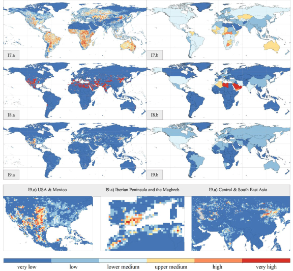
Figure 3. Results for the indicators I7–I9 (a: grid-cell based results; b: country-based results based on consumption-weighted averages); all indicators are dimensionless and represent a value between zero and one; no data values are marked in grey colour; in the following, indicator names and class thresholds for determining very low to very high risks are listed: I7) GDE probability [0, 0.05, 0.14, 0.23, 0.35, 0.52, 1]; I8) groundwater stress [0, 0.25, 0.5, 0.63, 0.75, 0.88, 1]; I9) risk index (I7*I8) [0, 0.01, 0.07, 0.15, 0.26, 0.45, 1]; the lower part of the figure shows exemplary enlarged image sections for grid cells where GDEs may be at risk (I9.a).
Download figure:
Standard image High-resolution image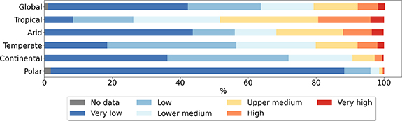
Figure 4. Percentage distribution of GDE probability classes according to primary climate zones and on global average.
Download figure:
Standard image High-resolution imageSecondly, groundwater stress per grid cell is shown (I8.a in figure 3). Accumulations of cells with very high groundwater stress are found in the US, Mexico, Chile, Southern Europe, the Middle East, India as well as China and Mongolia. This trend is mostly in line with hotspots found in previous studies (Gleeson et al 2012, Wada and Bierkens 2014, IGRAC 2020).
Combining groundwater stress with GDE probabilities finally enabled the identification of risks for GDEs induced by groundwater abstraction (I9.a in figure 3). Hotspots are shown enlarged and refer to the US and Mexico, the Maghreb and the Iberian Peninsula as well as Central, South and East Asia. Within the US, it is mainly the states located towards the border with Mexico as well as centrally located states that show an increased number of grid cells with high to very high risks. In Mexico, mainly the northern border regions and the centrally located metropolitan region around Mexico City are critical. As for the Iberian Peninsula and the Maghreb, Southern Spain, Central Morocco and Tunisia contain potential hotspots, while in Asia these are found in Turkmenistan, Uzbekistan, Kazakhstan, India and the North-East of China. The hotspots identified coincide with typical regions that are studied as example regions in the context of GDE research or groundwater management (USA: Howard et al (2010) and Gou et al (2015); Spain: Páscoa et al (2020); the Maghreb: Hirich et al (2017); Central Asia: Liu et al (2021); North China: Currell et al (2012) and Wang et al (2015)).
Regarding the sensitivity of identified risks to increasing groundwater consumption and varying EFRs, the scenario analysis in figure 5 allows the following conclusions: while in the baseline scenario (scenario 1–EFR = 60%) only 1.6% of grid cells show risks for GDEs in the upper medium or higher range, these increase to 2.3% and 3.1% for abstraction scenarios 2 and 3, respectively, assuming no change in the EFR. The related plots in S12 show that with increasing abstraction, risk mostly intensifies in already known risk regions without spreading to other regions extensively. However, when raising the EFR to 90%, risks spread spatially more strongly and almost 6% of grid cells reach upper medium or higher risk ranges (figure 5). Where previously there were no or only few isolated risk regions, new hotspots cover the East of the US, Cuba, North-East Brazil, Northern Argentina, savannahs north of the Central-African tropics, East and South Africa, and areas North-West of the Caspian Sea (S12). The sensitivity analysis of I7 to I9 to the number of classes showed in parallel that the proportions of cells linked to low, medium or high attributes may vary slightly, but that basic spatial distribution patterns remain consistent (S13).

Figure 5. Share of grid cells in % with upper medium to higher risks for GDEs (I9.a) in different scenarios; scenario 1 corresponds to current average net groundwater abstraction; scenario 2 considers increases in water abstraction as expected until 2050 based on past trends; scenario 3 simulates an increase of water consumption by 100%; all scenarios take into account different environmental flow requirements (EFRs) covering 0%, 30%, 60% and 90% of the average groundwater recharge; the baseline scenario of our work (Scenario 1—EFR = 60%) is highlighted in blue font and increases in total water consumption in scenarios 2 and 3 were fully allocated to groundwater.
Download figure:
Standard image High-resolution image
Aggregated at country level, the indicator results represent average risks in relation to the spatial distribution of (ground)water consumption. Considering the mere co-existence of consumption and GDEs, the probability is highest in countries such as the Central African Republic, South Sudan and Botswana (I7.b in figure 3). Regarding groundwater stress as such, the countries of the Arabian Peninsula and Libya pose greatest risks (I8.b in figure 3). However, when combining both perspectives, risks in the upper medium or higher range become indistinct at country scale (I9.b in figure 3). This is because GDEs, groundwater stress and (ground)water consumption often do not occur simultaneously across larger territories.
3.4. Implications
Implications of our work are twofold: general applications for the research field of GDEs directly, and implications for sustainability-related tools discussed using the water footprint. Regarding the first, indicators I1 to I3 can be used for research whenever potentials for global distribution patterns on different GDE types are of interest. This is complemented by information on GDE diversity (I4) and land covers relevant to GDEs (I5). High overall GDE potentials (I6) were identified in tropical regions that are usually not the focus of established GDE research. This could be a stimulus for future research to better understand such systems. Also, our work may be used to prioritise regions for regional GDE studies based on more site-specific data collection and high-resolution remote sensing imagery. In this context, priorities could be set to cover regions where GDEs are potentially at risk. Although previous research already partially covers these regions, our work could serve as an impetus for further analysis and GDE conservation strategies with respect to them.
Implications for water footprinting are as follows: indicators I7–I9 can be used to characterise potential ecosystem threats related to groundwater consumption in global product systems. Since global groundwater inventories may often not be available at high spatial resolution, the derived country factors may be useful for first operationalisation. However, practitioners should be aware of the drawback that risks may become indistinct due to heterogeneous distribution patterns of GDEs, groundwater stress and (ground)water consumption across countries. Whenever possible, watershed resolution or, in the best case, results at grid cell level should be preferred. The developed factors can be applied in two ways: firstly, groundwater consumption along the supply chain can be assigned to the individual risk classes of indicators I7 to I9 and needs for action may be derived. This can mean, for instance, that potential hotspots in the supply chain are verified through more detailed local analyses, and if they persist, water stewardship measures for the improvement of local conditions are initiated (Berger et al 2021). Secondly, numerical values behind risk classes may be used to weight the severity of groundwater consumption. Multiplying these by each associated consumption and summing the individual components, gives a single numerical value per product system which, the higher it is, implies a higher potential risk for GDEs. This use corresponds to the use of characterisation factors in water footprinting (ISO 14046 2016), which convert water consumption at a specific region into a comparable impact-related quantity. In this context, the application of indicators I7 to I9 represents different use cases. I7 may be used as a conservative measure to indicate risks based only on the co-existence of GDEs and groundwater consumption. I8 considers groundwater stress as such, while I9 combines both perspectives. We stress that I7 and I9 consider the land cover share of natural ecosystems relevant to GDEs. Thus, no potential impacts are displayed where ecosystems have been converted into cropland or urban land. This could be regarded as critical from a sustainability point of view, as regions that are far from their natural state tend to be viewed more positively. Therefore, in holistic considerations, the effects of land cover changes should be considered separately. Another limitation of our method is that it focuses exclusively on anthropogenic pressures on GDEs from groundwater extraction. However, in reality, various other pressures such as water abstraction from other compartments and its associated effects on groundwater, groundwater pollution or climate change impacts pose a potential threat to GDEs (Erostate et al 2020). In addition, should global data availability improve, we recommend that future studies include GDE types not considered in this work, such as spring, cave, and estuarine ecosystems. It should also be noted that further work is needed to determine specific and spatially differentiated ERFs for different GDE types. Finally, we underline that the factors developed can describe potential risks for GDEs induced by groundwater abstraction, but not the actual extent of ecosystem damages. This would require models that are based more heavily on cause-effect chain modelling and incorporate information on ecosystem resilience and adaptive capacity. Nevertheless, the indices provided could be used as a proxy for the description of potential impacts until more sophisticated global models are available.
Acknowledgments
The authors thank the following institution for funding of this research: the German Research Foundation (DFG) (Project Number: FI 1622/4-1). Additionally, we thank Jenny Brown, Patrícia Páscoa and Chan Liu for providing comparative study outputs for validation.
Data availability statement
The data that support the findings of this study are openly available at the following URL/DOI: https://data.mendeley.com/datasets/p39y3mdh6n/3. This includes all key results (indicators I1 to I9) and processed input data (S14).
Authors' contributions
A L: lead regarding conceptualisation, data curation, formal analysis, validation, visualisation and original draft preparation; all authors contributed to the conceptualisation, supervision and review and editing process; R R: provision of data from the models WaterGAP2d and G3M; M B and M F: funding acquisition
Conflict of interest
The authors declare no conflict of interest.
Supplementary data (4.9 MB PDF)