Abstract
We summarize important recent advances in quantum metrology, in connection to experiments in cold gases, trapped cold atoms and photons. First we review simple metrological setups, such as quantum metrology with spin squeezed states, with Greenberger–Horne–Zeilinger states, Dicke states and singlet states. We calculate the highest precision achievable in these schemes. Then, we present the fundamental notions of quantum metrology, such as shot-noise scaling, Heisenberg scaling, the quantum Fisher information and the Cramér–Rao bound. Using these, we demonstrate that entanglement is needed to surpass the shot-noise scaling in very general metrological tasks with a linear interferometer. We discuss some applications of the quantum Fisher information, such as how it can be used to obtain a criterion for a quantum state to be a macroscopic superposition. We show how it is related to the speed of a quantum evolution, and how it appears in the theory of the quantum Zeno effect. Finally, we explain how uncorrelated noise limits the highest achievable precision in very general metrological tasks.
This article is part of a special issue of Journal of Physics A: Mathematical and Theoretical devoted to '50 years of Bell's theorem'.
Export citation and abstract BibTeX RIS

Content from this work may be used under the terms of the Creative Commons Attribution 3.0 licence. Any further distribution of this work must maintain attribution to the author(s) and the title of the work, journal citation and DOI.
1. Introduction
Metrology plays a central role in science and engineering. In short, it is concerned with the highest achievable precision in various parameter estimation tasks, and with finding measurement schemes that reach that precision. Originally, metrology was focusing on measurements using classical or semiclassical systems, such as mechanical systems described by classical physics or optical systems modelled by classical wave optics. In the last decades, it has become possible to observe the dynamics of many-body quantum systems. If such systems are used for metrology, the quantum nature of the problem plays an essential role in the metrological setup. Examples of the case above are phase measurements with trapped ions [1], inteferometry with photons [2–5] and magnetometry with cold atomic ensembles [6–11].
In this paper, we review various aspects of quantum metrology with the intention to give a comprehensive picture to scientists with a quantum information science background. We will present simple examples that, while can be used to explain the fundamental principles, have also been realized experimentally. The basics of quantum metrology [12–21] can be perhaps best understood in the fundamental task of magnetometry with a fully polarized atomic ensemble. It is easy to deduce the precision limits of the parameter estimation, as well as the methods that can improve the precision. We will also consider phase estimation with other highly entangled states such as for example Greenberger–Horne–Zeilinger (GHZ) states [22].
After discussing concrete examples, we present a general framework for computing the precision of the parameter estimation in the quantum case, based on the Cramér–Rao bound and the quantum Fisher information. In the many-particle case, most of the metrology experiments have been done in systems with simple Hamiltonians that do not contain interaction terms. Such Hamiltonians cannot create entanglement between the particles. For cold atoms, a typical situation is that the input state is rotated with some angle and this angle must be estimated. We will show that quantum states with particles exhibiting quantum correlations, or more precisely, quantum entanglement [23, 24], provide a higher precision than an ensemble of uncorrelated particles. The most important question is how the achievable precision  scales with the number of particles. Very general derivations lead to, at best,

for non-entangled particles. Equation (1) is called the shot-noise scaling, the term originating from the shot-noise in electronic circuits, which is due to the discrete nature of the electric charge. θ is a parameter of a very general unitary evolution that we would like to estimate. On the other hand, quantum entanglement makes it possible to reach

which is called the Heisenberg-scaling. Note that if the Hamiltonian of the dynamics has interaction terms then even better scaling is possible (see, e.g., [25–31]).
All the above calculations have been carried out for an idealized situation. When a uncorrelated noise is present in the system, it turns out that for large enough particle numbers the scaling becomes a shot-noise scaling. The possible survival of a better scaling under correlated noise, under particular circumstances, or depending on some interpretation of the metrological task, is at the centre of attention currently. All these are strongly connected to the question of whether strong multipartite entanglement can survive in a noisy environment.
Our paper is organized as follows. In section 2, we will discuss examples of metrology with large particle ensembles and show simple methods to obtain upper bounds on the achievable precision. In section 3, we define multipartite entanglement and discuss how entanglement is needed for spin squeezing, which is a typical method to improve the precision of some metrological applications in cold gases. We also discuss some generalized spin squeezing entanglement criteria. In section 4, we introduce the Cramér–Rao bound and the quantum Fisher information, and other fundamental notions of quantum metrology. In section 5, we show that multipartite entanglement is a prerequisite for maximal metrological precision in many very general metrological tasks. We also discuss how to define macroscopic superpositions, how the entanglement properties of the quantum state are related to the speed of the quantum mechanical processes and to the quantum Zeno effect. We will also very briefly discuss the meaning of inter-particle entanglement in many-particle systems. In section 6, we review some of the very exciting recent findings showing that uncorrelated noise can change the scaling of the precision with the particle number under very general assumptions.
2. Examples for simple metrological tasks with many-particle ensembles
In this section, we present some simple examples of quantum metrology, involving an ensemble of N spin- particles in an external magnetic field. We demonstrate how simple ideas of quantum metrology can help to determine the precision of some basic tasks in parameter estimation. We consider completely polarized ensembles, as well as GHZ states, symmetric Dicke states [10, 32–34] and singlet states [35, 36].
First, let us explain the characteristics of the physical system we use for our discussion. In a large particle ensemble, typically only collective quantities can be measured. For spin- particles, such collective quantities are the angular momentum components defined as
for  where
where  are the components of the angular momentum of the
  particle. More concretely, we can measure the expectation values and the variance of the angular momentum component
  where
where  is a unit vector describing the component.
The typical Hamiltonians involve also collective observables, such as the Hamiltonian describing the action of a magnetic field pointing in the  -direction

where γ is the gyromagnetic ratio, B is the strength of the magnetic field,  is the direction of the field, and
  is the angular momentum component parallel with the field. Hamiltonians of the type (4) do not contain interaction terms, thus starting from a product state we arrive also at a product state. Interferometry with dynamics determined by (4) is discussed in the context of SU(2) interferometers [37], as the Jl are the generators of the SU(2) group. We will mostly study this type of interferometry in multiparticle systems, as it gives a good opportunity to relate the entanglement of many-particle states to their metrological performance.
The Hamiltonian (4), with the choice of  generates the dynamics

where we defined the angle θ that depends on the evolution time t

A basic task in quantum metrology is to estimate the small parameter θ by measuring the expectation value of a Hermitian operator, which we will denote by M in the following. If the evolution time t is a constant then estimating θ is equivalent to estimating the magnetic field  The precision of the estimation can be characterized with the error-propagation formula as
where  is the expectation value of the operator
  and its variance is given as

Thus, the precision of the estimate depends on how sensitive  is to the change of
  and also on how large the variance of M is. Based on the formula (7), one can see that the larger the slope
  the higher the precision. On the other hand, the larger the variance
  the lower the precision.
The formula (7) above can be calculated for any given  Thus, this formalism can be used to characterize small fluctuations around a given
  For simplicity we will calculate the precision typically for
  (To be more precise, if both the numerator and the denominator in (7) are zero, then we will take the
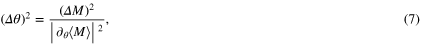
  limit instead.) This approach is connected to the estimation theory based on the quantum Fisher information discussed in this review and could be called a local approach. Figure 1 helps to interpret the quantities appearing in (7). We note that the global alternative is the Bayesian estimation theory. There, the parameter to be estimated is a random variable with a certain probability density
  For a recent review discussing this approach in detail, see [19]. For an application, see [38].
Figure 1. Calculating the precision of estimating the small parameter θ based on measuring M given by the error propagation formula (7). Solid curve: the expectation value  as a function
  Dashed curves: uncertainty of M as a function of θ given as a confidence interval. Vertical arrow: the uncertainty
  for
for  Dashed line: tangent of the curve
  at
at  Its slope is
  Horizontal arrow:
  is the uncertainty of the parameter estimation.
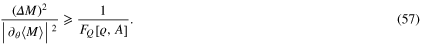
Download figure:
Standard image High-resolution imageFinally, note that often, instead of  one calculates
  which is large for a high precision. It scales as
  for the shot-noise scaling, and as ∼N2 for the Heisenberg scaling. (Compare with (1) and (2).)
2.1. Ramsey-interferometry with spin squeezed states
Let us start with a basic scheme for magnetometry using an almost completely polarized state. The total spin of the ensemble, originally pointing into the z-direction, is rotated by a magnetic field pointing to the y-direction, as can be seen in figure 2(a). Hence, the unitary giving the dynamics of the system is

The stronger the field, the faster the rotation. The rotation angle can be obtained by measuring  a spin component perpendicular to the initial spin. The estimation of rotation angle in such an experiment is a particular case of Ramsey-interferometry (see, e.g., [13, 19]) and has been realized for magnetometry in cold atoms [39]. This idea has been used in experiments with cold gases to get even a spatial information on the magnetic field and its gradient [6–9, 11].
Figure 2. (a) Magnetometry with an ensemble of spins, all pointing into the z direction. Solid arrow: the large collective spin precesses around the magnetic field pointing into the y direction. Dashed arrow: after a precession of an angle  the uncertainty ellipse of the spin is not overlapping with the uncertainty ellipse of the spin at the starting position. Hence,
  is close to the uncertainty of the phase estimation, which coincides with the shot-noise limit. (b) Magnetometry with an ensemble of spins, all pointing to the z direction and spin squeezed along the x direction. The uncertainty of the phase estimation is close to the angle
  which is smaller than
  due to the spin squeezing.
Download figure:
Standard image High-resolution imageSo far, it looks as if the mean spin behaves like a clock arm and its position tells us the value of the magnetic field. At this point one has to remember that we have an ensemble of particles governed by quantum mechanics, and the uncertainty of the spin component perpendicular to the mean spin is not zero. For the completely polarized state, the squared uncertainty is

Hence, the angle of rotation can be estimated only with a finite precision as can be seen in figure 2(a). Intuitively speaking, we can detect a rotation θ only if the uncertainty ellipses of the spin in the original position and in the position after the rotation do not overlap with each other too much. Based on these ideas and (10), with elementary geometric considerations, we arrive at
Thus, we obtained the shot-noise scaling (1), even with very simple, qualitative arguments.
A more rigorous argument is based on the formula (7), where we measure the operator

The expectation value and the variance of this operator, as a function of  are
are
Hence, using  , we obtain for the precision
which equals  demonstrating a shot-noise scaling for the totally polarized states.
We can see that  could be smaller if we decrease
  [40]. A comparison between figures 2(a) and (b) also demonstrates the fact that a smaller
  leads to a higher precision. The variances of the angular momentum components are bounded by the Heisenberg uncertainty relation [41]

Thus, the price of decreasing  is increasing
Let us now characterize even quantitatively the properties of the state that can reach an improved metrological precision. For fully polarized states, (15) is saturated such that

Due to decreasing  , our state fulfils

where z is the direction of the mean spin, and the bound in (17) is the square root of the bound in (15). Such states are called spin squeezed states [41–44]. In practice this means that the mean angular momentum of the state is large, and in a direction orthogonal to the mean spin the uncertainty of the angular momentum is small. An alternative and slightly different definition of spin squeezing considers the usefulness of spin squeezed states for reducing spectroscopic noise in a setup different from the one discussed in this section [42]. Spin squeezing has been realized in many experiments with cold atomic ensembles. In some systems the particles do not interact with each other, and light is used for spin squeezing [13, 39, 45–48], while in Bose–Einstein condensates the spin squeezing can be generated using the inter-particle interaction [11, 49–51].
Next, we can ask, what the best possible phase estimation precision is for the metrological task considered in this section. For that, we have to use the following inequality based on general principles of angular momentum theory

Note that equation (18) is saturated only by symmetric multiqubit states. Together with the identity connecting the second moments, variances and expectation values

equation (18) leads to a bound on the uncertainty in the squeezed orthogonal direction

Introducing the maximal spin length

we arrive at the inequality

This leads to a simple bound on the precision
which indicates that the precision is limited for almost completely polarized spin squeezed states with  Here, the equality in (23) is based on (14), while the first inequality is due to (15), and the second one comes from (22). The bound in (23) is not optimal, as for the fully polarized state we would expect
  while (23) allows for a higher precision for
It is possible to obtain the best achievable precision numerically for our case, when  is measured for a state that is almost completely polarized in the z-direction in a field pointing into the y-directon. For even
  states giving the smallest
  for a given
  can be obtained as a ground state of the Hamiltonian [43]

where  plays the role of a Lagrange multiplier. This also means that the ground states of
  give the best
  for a given
  when collective operators are measured for estimating θ. Since the ground state of (24) is symmetric, it is possible to make the calculations in the symmetric subspace and hence model large systems. We plotted the precision
  as a function of the polarization
  for different values of N in figure 3, which demonstrates that
  scales as
  Hence, for the precision of phase-estimation the Heisenberg scaling (2) can be reached.
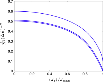
Figure 3. The best precision achievable (14) divided by N2 as the function of the total spin, from top to bottom, for  particles. The curves converge to the same curve for large
  which demonstrates an N2 scaling for the precision. Note that the maximum appears in the limit in which the spin length is zero.
Download figure:
Standard image High-resolution imageParadoxically the maximum is reached in the limit of zero mean spin. An added noise can radically change this situation. If the mean spin is small, and its direction is the information that we use for metrology, then a very small added noise can change the direction of the spin, making the metrology for this case impractical. Thus, if we consider local noise acting on each particle independently, then the maximum  will be reached at a finite spin length.
2.2. Metrology with a GHZ state
Next, we will show another example where the Heisenberg scaling for the precision of phase estimation can be reached. The scheme is based on a GHZ state defined as

where we follow the usual convention defining the  and
and  states with the eigenstates of jz as
  and
and  Such states have been created in photonic systems [52–56] and in cold trapped ions [1, 57, 58]. Let us consider the dynamics given by

Under such dynamics, the GHZ state evolves as

hence the difference of the phases of the two terms scales as  Let us consider measuring the operator

which is essentially the parity in the x-basis. Note that this operator needs an individual access to the particles. For the dynamics of the expectation value and the variance we obtain

Hence, based on (7), for small θ the precision is

which means that we reached the Heisenberg scaling (2). In [1], the scheme described above has been realized experimentally with three ions and a precision above the shot-noise limit has been achieved.
Note, however, that the GHZ state is very sensitive to noise. Even if a single particle is lost, it becomes a separable state. Thus, it is a very important question, how well such a state can be created, and how noise is influencing the scaling of the precision with the particle number. This question will be discussed in section 6. Concerning spin squeezed states and GHZ states, it has been observed that under local noise, such as dephasing and particle loss, for large particle numbers, the GHZ state becomes useless while the spin squeezed states, discussed in the previous section, are optimal [59].
A related metrological scheme for two-mode systems is based on a Mach–Zender interferometer [60–66], using as inputs NOON states defined as [18]

Here, the state  describes a system with n1 particles in the first bosonic mode and n2 particles in the second bosonic mode. For example, the two modes can be two optical modes, or, two spatial modes in a double-well potential. Thus, similarly to GHZ states, the state is a superposition of two states: all particles in the first state and all particles in the second state. However, in this scheme we do not have a local access to the particles. Hence, we cannot easily measure the operator (28), which is a multi-particle correlation operator, and instead the following operator has to be measured

The basic idea of the N-fold gain in precision is similar to the idea used for the method based on the GHZ state. The expectation value of M and the variance of M as a function of θ is the same as before, given in (29). With that, the Heisenberg scaling can be reached. Metrological experiments with NOON states have been carried out in optical systems that surpassed the shot-noise limit [2–5].
2.3. Metrology with a symmetric Dicke state
As a third example, we will consider metrology with N-qubit symmetric Dicke states
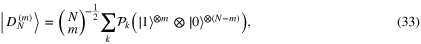
where the summation is over all the different permutations of m 1ʼs and  0ʼs. One of such states is the W-state for which
  which has been prepared with photons and ions [67, 68].
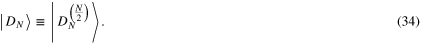
From the point of view of metrology, we are interested mostly in the symmetric Dicke state for even N and  This state is known to be highly entangled [69]. In the following, we will omit the superscript giving the number of 1ʼs and use the notation
Symmetric Dicke states of the type (34) have been created in photonic systems [33, 70–73] and in cold gases [10, 34, 74]. In reference [10, 72], their metrological properties have also been verified.
The state (34) has  for all
  For the second moments we obtain

It can be seen that  is minimal,
  and
and  are close to the largest possible value,
The state has a rotational symmetry around the z axis. Thus, the state is not changed by dynamics of the type  Based on these considerations, we will use dynamics of the type (9). Moreover, since the total spin length is zero, a rotation around any axis remains undetected if we measure only the expectation values of the collective angular momentum components. Hence, our setup will measure the expectation value of

Note that this is also a collective measurement. In practice, to measure  we have to measure Jz many times and compute the average of the squared values.
For the dynamics of the expectation value we obtain

The expectation value  starts from zero, and oscillates with a frequency twice as large as the frequency of the oscillation was for the analogous case for
  in (13). This is due to fact that after a rotation with an angle π we obtain again the original Dicke state. Following the calculations given in reference [10], we arrive at

which again means that we reached the Heisenberg scaling (2). The quantum dynamics of the Dicke state used for metrology is depicted in figure 4.
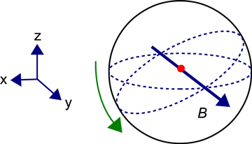
Figure 4. Magnetometry with Dicke states of the form (34). The uncertainty ellipse of the state is rotated around the magnetic field pointing to the x-direction. The rotation angle can be estimated by measuring the uncertainty of the z-component of the collective spin. Note that, unlike in the case of a fully polarized state, after a rotation of an angle π we obtain the original Dicke state.
Download figure:
Standard image High-resolution image2.4. Singlet states
Finally, we show another example for states that can be used for metrology in large particle ensembles. Pure singlet states are simultaneous eigenstates of Jl for  with an eiganvalue zero, that is,

Mixed singlet states are mixtures of pure singlet states, and hence  for any direction
  and any power
  Such states can be created in cold atomic ensembles by squeezing the uncertainties of all the three collective spin components [35, 75, 76]. Since in large systems practically all initial states and all the possible dynamics are permutationally invariant, they are expected to be also permutationally invariant. For spin-
 particles, there is a unique permutationally invariant singlet state [36]

where the summation is over all permutation operators Πk and

A realization of the singlet state (40) with an ensemble of particles is shown in figure 5.

Figure 5. For spin- particles, the permutationally invariant singlet is an equal mixture of all possible arrangements of two-particle singlets. Three of such arrangements are shown for eight particles. Note that the eight atoms are arranged in the same way on the figures, only the pairings are different.
Download figure:
Standard image High-resolution imageA singlet state is invariant under  for any
  Thus, it is completely insensitive to rotations around any axis. How can it be useful for magnetometry? Let us now assume that we would like to analyse a magnetic field pointing in the y-direction using spins placed in an equidistant chain. While the singlet (40) is insensitive to the homogenous component of the magnetic field, it is very sensitive to the dynamics

where  is proportional to the field gradient. This makes the state useful for differential magnetometry, since singlets are insensitive to external homogeneous magnetic fields, while sensitive to the gradient of the magnetic field [36]. Similar ideas work even if the atoms are in a cloud rather than in a chain. The quantity to measure in order to estimate
  is again
  as was the case in section 2.3. This idea is also interesting even for a bipartite singlet of two large spins [77].
3. Spin squeezing and entanglement
As we have seen in section 2.1, spin squeezed states have been more useful for metrology than fully polarized product states. Moreover, states very different from product states, such as GHZ states and Dicke sates could reach the Heisenberg limit in parameter estimation. Thus, large quantum correlations, or entanglement, can help in metrological tasks. In this section, we will discuss some relations between entanglement and spin squeezing, showing why entanglement is necessary to surpass the shot-noise limit. We also discuss that not only entanglement, but true multipartite entanglement is needed to reach the maximal precision in the metrology with spin squeezed states.
3.1. Entanglement and multi-particle entanglement
Next, we need the following definition. A quantum state is (fully) separable if it can be written as [78]

where  are single-particle pure states. Separable states are essentially states that can be created without an inter-particle interaction, just by mixing product states. States that are not separable are called entangled. Entangled states are more useful than separable ones for several quantum information processing tasks, such as quantum teleportation, quantum cryptography, and, as we will show later, for quantum metrology [23, 24].
In the many-particle case, it is not sufficient to distinguish only two qualitatively different cases of separable and entangled states. For example, an N-particle state is entangled, even if only two of the particles are entangled with each other, while the rest of the particles are, say, in the state  Usually, such a state we would not call multipartite entangled. This type of entanglement is very different from the entanglement of a GHZ state (25).
Hence, the notion of genuine multipartite entanglement [57, 79] has been introduced to distinguish partial entanglement from the case when all the particles are entangled with each other. It is defined as follows. A pure state is biseparable, if it can be written as a tensor product of two multi-partite states

A mixed state is biseparable if it can be written as a mixture of biseparable pure states. A state that is not biseparable, is genuine multipartite entangled. In many quantum physics experiments the goal was to create genuine multipartite entanglement, as this could be used to demonstrate that something qualitatively new has been created compared to experiments with fewer particles [33, 52–58, 70, 71, 73].
In the many-particle scenario, further levels of multi-partite entanglement must be introduced as verifying full N-particle entanglement for N = 1000 or 106 particles is not realistic. In order to characterize the different levels of multipartite entanglement, we start first with pure states. We call a state k-producible, if it can be written as a tensor product of the form

where  are multiparticle states with at most k particles. A k-producible state can be created in such a way that only particles within groups containing not more than k particles were interacting with each other. This notion can be extended to mixed states by calling a mixed state k-producible if it can be written as a mixture of pure k-producible states. A state that is not k-producible contains at least
  -particle entanglement [80, 81]. Using another terminology, we can also say that the entanglement depth of the quantum state is larger than k [43].
It is instructive to depict states with various forms of multipartite entanglement in set diagrams as shown in figure 6. Separable states are a convex set since if we mix two separable states, we can obtain only a separable state. Similarly, k-producible states also form a convex set. In general, the set of k-producible states contain the set of l-producible states if 
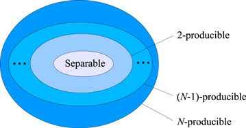
Figure 6. Sets of states with various forms of multipartite entanglement. k-producible states form larger and larger convex sets, 1-producible states being equal to the set of separable states, while the set of physical quantum states is equal to the set of N-producible states.
Download figure:
Standard image High-resolution image3.2. The original spin squeezing criterion
Let us see now how entanglement and multiparticle entanglement is related to spin squeezing. It turns out that spin squeezing, discussed in section 2.1, is strongly related to entanglement. A ubiquitous entanglement criterion in this context is the spin squeezing inequality [82]
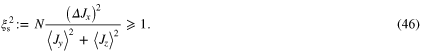
If a state violates (46), then it is entangled (i.e., not fully separable). In order to violate (46), its denominator must be large while its numerator must be small, hence, it detects states that have a large spin in some direction, while a small variance of a spin component in an orthogonal direction. That is, (46) detects the entanglement of spin squeezed states depicted in figure 2(b).
For spin squeezed states, it has also been noted that multipartite entanglement, not only simple nonseparability is needed for large spin squeezing [43]. To be more specific, for a given mean spin length, larger and larger spin squeezing is possible only if the state has higher and higher levels of multipartite entanglement. Moreover, larger and larger spin squeezing leads to larger and larger measurement precision. Such strongly squeezed states have been created experimentally in cold gases and a 170-particle entanglement has been detected [83].
At this point note that only the first and second moments of the collective quantities are needed to evaluate the spin squeezing condition (46). It is easy to show that all these can be obtained from the average two-particle density matrix of the quantum state defined as [84]

where ϱmn is the reduced two-particle state of particles m and 
In summary, entangled states seem to be more useful than separable ones for magnetometry with spin squeezed states discussed in section 2.1. Moreover, states with k-particle entanglement can be more useful than states with  -particle entanglement for the same metrological task. This finding will be extended to general metrological tasks in section 5.
3.3. Generalized spin squeezing criteria
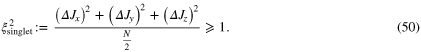
The original spin squeezing entanglement criterion (46) can be used to detect the entanglement of almost completely polarized spin squeezed states. However, there are other highly entangled states, such as Dicke states (34) and singlet states defined in (39). For these states, the denominator of the fraction in (46) is zero, thus they are not detected by the original squeezing entanglement criterion.
A complete set of entanglement conditions similar to the condition (46) has been determined, called the optimal spin squeezing inequalities. They are called optimal since, in the large particle number limit, they detect all entangled states that can be detected based on the first and second moments of collective angular momentum components. For separable states of the form (43), the following inequalities are satisfied [84]


where  take all the possible permutations of
  The inequality (48a
), identical to (18), is valid for all quantum states. On the other hand, violation of any of the inequalities (48b–48d) implies entanglement.
The inequality (48a
), identical to (18), is valid for all quantum states. On the other hand, violation of any of the inequalities (48b–48d) implies entanglement.
Based on the entanglement conditions (48), new spin squeezing parameters have been defined. For example, (48c ) is equivalent to [85]
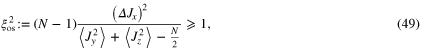
provided that the denominator of (49) is positive. The criterion (49) can be used to detect entanglement close to Dicke states, discussed in section 2.3. One can see that for the Dicke state (34), the numerator of the fraction in (49) is zero, while the denominator is maximal (see (35)). Apart from entanglement, it is also possible to detect multiparticle entanglement close to Dicke states. A condition linear in expectation values and variances of collective observables has been presented in [86] for detecting multipartite entanglement. A nonlinear criterion is given in [74], which detects all states as multipartite entangled that can be detected based on the measured quantities. The criterion has been used even experimentally [74]. An entanglement depth of 28 particles has been detected in an ensemble of around 8000 cold atoms.
The inequality (48b ) is equivalent to [35, 76]
The parameter  can be used to detect entanglement close to singlet states discussed in section 2.4. It can be shown that the number of non-entangled spins in the ensemble is bounded from above by
Finally, it is interesting to ask, what the relation of the new spin squeezing parameters is to the original one. It can be proved that the parameters  and
and  detect all entangled states that are detected by
  They detect even states not detected by
  such as entangled states with a zero mean spin, like Dicke states and singlet states. Moreover, it can be shown that for large particle numbers,
  in itself is also strictly stronger than
  [85].
[85].
4. Quantum Fisher information
In this section, we review the theoretical background of quantum metrology, such as the Fisher information, the Cramér–Rao bound and the quantum Fisher information.
4.1. Classical Fisher information
Let us consider the problem of estimating a parameter θ based on measuring a quantity  Let us assume that the relationship between the two is given by a probability density function
  This function, for every value of the parameter
  gives a probability distribution for the x values of
Let us now construct an estimator  which would give for every value x of M an estimate for
  In general it is not possible to obtain the correct value for θ exactly. We can still require that the estimator be unbiased, that is, the expectation value of
  should be equal to θ. This can be expressed as

How well the estimator can estimate θ? The Cramér–Rao bound provides a lower bound on the variance of the unbiased estimator as

where the Fisher information is defined with the probability distribution function  as
as

The inequality (52) is a fundamental tool in metrology that appears very often in physics and engineering, and can even be generalized to the case of quantum measurement. Finally, note that the inequality (52) is giving a lower bound for parameter estimation in the vicinity of a given  This is the local approach discussed in section 2.
4.2. Quantum Fisher information
In quantum metrology, as can be seen in figure 7, one of the basic tasks is phase estimation connected to the unitary dynamics of a linear interferometer

where ϱ is the input state,  is the output state, and A is a Hermitian operator. The operator A can be, for example, a component of the collective angular momentum
  The important question is, how well we can estimate the small angle θ by measuring

Figure 7. The basic problem of linear interferometry. The parameter θ must be estimated by measuring 
Download figure:
Standard image High-resolution imageLet us use the notion of Fisher information to quantum measurements assuming that the estimation of θ is done based on measuring the operator  Let us denote the projector corresponding to a given measured value x by
  Then, we can write

which can be used to define an unbiased estimator based on (51). Then, the Fisher information can be obtained using (53). Finally, using (55), the Cramér–Rao bound (52) gives a lower bound on the precision of the estimation. A similar formalism works even if the measurements are not projectors, but in the more general case, positive operator valued measures (POVM).
We could calculate a bound for the precision of the estimation for given dynamics and a given operator to be measured using this formalism. However, it might be difficult to find the operator that leads to the best estimation precision just by trying several operators. Fortunately, it is possible to find an upper bound on the precision of the parameter estimation that is valid for any choice of the operator. The phase estimation sensitivity, assuming any type of measurement, is limited by the quantum Cramér–Rao bound as [87, 88]

where FQ is the quantum Fisher information. As a consequence, based on (7), for any operator M we have
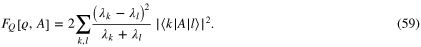
The quantum Fisher information FQ can be computed easily with a closed formula. Let us assume that a density matrix is given in its eigenbasis as

Then, the quantum Fisher information is given as [87–90]
Next, we will review some fundamental properties of the quantum Fisher information which relate it to the variance.
(i) For pure states, from (59) follows

(ii) For all quantum states, it can be proven that

This provides an easily computable upper bound on the quantum Fisher information.
For quantum states with  we obtain that
 ![${{F}_{Q}}[\varrho ,A]=0.$](https://content.cld.iop.org/journals/1751-8121/47/42/424006/revision1/jpa500438ieqn132.gif) Such a state does not change under unitary dynamics of the type
Such a state does not change under unitary dynamics of the type  It is instructive to consider the example when
  for
for  Then,
Then,  also implies that the state does not change under the dynamics
  as we could see in the case of the singlet states in section 2.4.
(iii) More generally, the quantum Fisher information is convex in the state, that is

(iv) Recently, it has turned out that the quantum Fisher information is the largest convex function that fulfils (i) [91, 92]. This can be stated in a concise form as follows. Let us consider a very general decomposition of the density matrix

where  and
and  With that, the quantum Fisher information can be given as the convex roof of the variance,

where the optimization is over all the possible decompositions (63).
At this point we have to note that if  in the decomposition (63) were pairwise orthogonal to each other, then the decomposition (63) would be an eigendecomposition. For density matrices with a non-degenerate spectrum, it would even be unique and easy to obtain by any computer program that diagonalizes matrices. However, the pure states
  are not required to be pairwise orthogonal, which leads to an infinite number of possible decompositions. Convex roofs over all such decompositions appear often in quantum information science [23, 24] in the definitions of entanglement measures, for example, the entanglement of formation [93, 94]. These measures can typically be computed only for small systems. Here, surprisingly, we have the quantum Fisher information given by a convex roof that can also be obtained as a closed formula (59) for any system sizes.
There are generalized quantum Fisher informations different from the original one (59). They are convex and have the same value for pure states as the quantum Fisher information does [91]. However, they cannot be larger than the quantum Fisher information. This is counterintuitive: the quantum Fisher information is defined with an infimum, still it is easy to show that it is the largest, rather than the smallest, among the generalized quantum Fisher informations. As an example, we mention one of the generalized quantum Fisher informations, defined as four times the the Wigner–Yanase skew information given as [95]

For pure states, ![$I[\varrho ,A]$](https://content.cld.iop.org/journals/1751-8121/47/42/424006/revision1/jpa500438ieqn142.gif) equals the variance and it is convex. There are even other types of generalized quantum Fisher informations. References [96, 97] introduce an entire family of generalized quantum Fisher informations, together with a family of generalized variances.
equals the variance and it is convex. There are even other types of generalized quantum Fisher informations. References [96, 97] introduce an entire family of generalized quantum Fisher informations, together with a family of generalized variances.
Analogously to (64), it can also be proven that the concave roof of the variance is itself [91]

Hence, the main statements can be summarized as follows. For any decomposition  of the density matrix ϱ we have

where the upper and the lower bounds are both tight in the sense that there are decompositions that saturate the first inequality, and there are others that saturate the second one4 .
Let us now discuss an alternative way to interpret the inequalities of (67), relating them to the theory of quantum purifications, which play a fundamental role in quantum information science. A mixed state ϱ with a decompostion (63) can be represented as a reduced state  of a pure state, called the purification of
  defined as

Here  is an orthogonal basis for the ancillary system, and
  denotes tracing out the ancilla. Note that all purification can be obtained from each other using a unitary acting on the ancilla. This way one can obtain purifications corresponding to all the various decompositions.
Let us now assume that a friend controls the ancillary system and can assist us to achieve a high precision with the quantum state, or can even hinder our efforts. Our friend can choose between the purifications with unitaries acting on the ancilla. Then, our friend makes a measurement on the ancilla, and sends us the result  This way we receive the states
  together with the label
  corresponding to some decomposition of the type (63). The average quantum Fisher information for the
  states is bounded from below and from above as given in (67). The worst case bound is given by the quantum Fisher information. We can always achieve this bound even if our friend acts against us.
On the other hand, if the friend acting on the ancilla helps us, a much larger average quantum Fisher information can be achieved, equal to four times the variance. At this point, there is a further connection to quantum information science. Besides entanglement measures defined with convex roofs, there are measures defined with concave roofs [100–102]. For example, the entanglement of assistance is defined as the maximum average entanglement that can be obtained if the party acting on the ancilla helps us. Thus, in quantum information language, the variance can be called the quantum Fisher information of assistance over four. Later, we will see another connection between purifications and the quantum Fisher information in section 6.
After the discussion relating the quantum Fisher information to the variance, and examining its convexity properties, we list some further useful relations for the quantum Fisher information. From (59), we can obtain directly the following identities.
(i) The formula (59) does not depend on the diagonal elements  Hence,

where D is a matrix that is diagonal in the basis of the eigenvectors of  i.e.,
i.e., ![$[\varrho ,D]=0.$](https://content.cld.iop.org/journals/1751-8121/47/42/424006/revision1/jpa500438ieqn154.gif)
(ii) The following identity holds for all unitary dynamics U

The left- and right-hand sides of (70) are similar to the Schrödinger picture and the Heisenberg picture, respectively, in quantum mechanics. Hence, in particular, the quantum Fisher information does not change under unitary dynamics governed by A as a Hamiltonian

(iii) The quantum Fisher information is additive under tensoring

For N-fold tensor product of the system, we obtain an N-fold increase in the quantum Fisher information
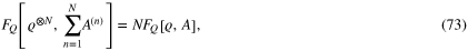
where  denotes the operator A acting on the
  subsystem.
(iv) The quantum Fisher information is additive under a direct sum [103]

where ϱk are density matrices with a unit trace and  Equation (74) is relevant, for example, for experiments where the particle number variance is not zero, and the ϱk correspond to density matrices with a fixed particle number [104, 105].
(v) If a pure quantum state  of N d-dimensional particles is mixed with white noise as [106, 107]

then
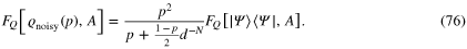
Thus, an additive global noise decreases the quantum Fisher information by a constant factor. If p does not depend on N then it does not influence the scaling of the quantum Fisher information with the number of particles. Note that this is not the case for a local uncorrelated noise. A constant uncorrelated local noise contribution can destroy the scaling of the quantum Fisher information and lead back to the shot-noise scaling for large  as will be discussed in section 6.
(vi) If we have a bipartite density matrix and we trace out the second system, the quantum Fisher information cannot increase (see, e.g. [108])

In fact, in many cases it decreases even if the operator A(1) was acting on the first subsystem, and thus the unitary dynamics changed only the first subsystem. This is due to the fact that measurements on the entire system can lead to a better parameter estimation than measurements on the first system. Let us see a simple example with the following characteristics
where  is defined in (41). Since
  is the completely mixed state, the right-hand side of the inequality (77) is zero, while the left-hand side is positive. On the other hand, (77) is always saturated if ϱ is a product state of the form
(vii) It is instructive to write the quantum Fisher information in an alternative form as [109]
(ix) Following a similar idea, equation (64) can also be rewritten as

By removing the second moments of the operator from the infimum, we make the optimization simpler.
Similarly, we can also rewrite the formula (66) as

(x) Finally, based on (80) and (81), the difference between the variance and the quantum Fisher information over four is obtained as

Clearly, (82) is zero for all pure states. It can also be zero for some mixed states. For example, based on (61), we see that for all states for which we have  we also have
 ![${{F}_{Q}}[\varrho ,A]=0.$](https://content.cld.iop.org/journals/1751-8121/47/42/424006/revision1/jpa500438ieqn164.gif) Thus, the difference (82) is also zero for such quantum states.
Thus, the difference (82) is also zero for such quantum states.
4.3. Optimal measurement
The Cramér–Rao bound (56) defines the achievable largest precision of parameter estimation, however, it is not clear what has to be measured to reach this precision bound. An optimal measurement can be carried out if we measure in the eigenbasis of the symmetric logarithmic derivative L [89, 90]. This operator is defined such that it can be used to describe the quantum dynamics of the system with the equation

Unitary dynamics are generally given by the von Neumann equation with the Hamiltonian A

The operator L can be found based on knowing that the right-hand side of (83) must be equal to the right-hand side of (84). Hence, the symmetric logarithmic derivative can be expressed with a simple formula as

where λk and  are the eigenvalues and eigenvectors, respectively, of the density matrix
  Based on (59) and (85), the symmetric logarithmic derivative can be used to obtain the quantum Fisher information as

For a pure state  the formula (85) can be simplified and the symmetric logarithmic derivative can be obtained as

It is instructive to consider a concrete example. Let us find L for the setup based on metrology with the fully polarized ensemble discussed in section 2.1. In this case,  and the quantum state evolves according to the equation

where the initial state is

For short times, the dynamics can be written as

Using the identity with 2 × 2 matrices

the short-time dynamics can be rewritten as

Hence, for this case the symmetric logarithmic derivative is

Indeed, in the example of section 2.1 we measured  which now turned out to be the optimal operator to be measured.
Let us now see what can be obtained from the explicit formula (87) for the symmetric logarithmic derivative. Together with (91), it leads to

As the example shows, (93) and (94) are different, hence L is not unique. Nevertheless, the right-hand side of (83) is the same for (93) and (94). This is because the symmetric logarithmic derivative is defined unambiguously within the support of  while in the orthogonal space it can take any form as long as (83) is satisfied.
4.4. Multi-parameter metrology
The formalism of section 4.2 can be generalized to the case of estimating several parameters. The Cramér–Rao bound for this case is

where the inequality in (95) means that the left-hand side is a positive semidefinite matrix, C is now the covariance matrix with elements

and F is the Fisher matrix. It is defined as for the case of a unitary evolution
where λk and  are the eigenvalues and eigenvectors of the density matrix
  respectively (see (58)).
The bound of (95) cannot always be saturated, as it can happen that the optimal measurement operators for the various θk parameters do not commute with each other. Examples of multiparameter estimation include estimating parameters of unitary evolution as well as parameters of dissipative processes, such as for example phase estimation in the presence of loss such that the loss is given [38], the estimation of both the phase and the loss [110], estimation of phase and diffusion in spin systems [111], joint estimation of a phase shift and the amplitude of phase diffusion at the quantum limit [112], the joint estimation of the two defining parameters of a displacement operation (i.e., x and p) in phase space [113], optimal estimation of the damping constant and the reservoir temperature [114], estimation of the temperature and the chemical potential characterizing quantum gases [115], estimation of two-parameter rotations in spin systems [116], and the simultaneous estimation of multiple phases [117]. Multiparameter estimation is considered in a very general framework in [118]. Note that not all from the examples discussed above carry out a multi-parameter estimation in the sense it was explained in this section.
5. Quantum Fisher information and entanglement
In this section, we review some important facts concerning the relation between the phase estimation sensitivity in linear interferometers and entanglement. We will show that entanglement is needed to overcome the shot-noise sensitivity in very general metrological tasks. Moreover, not only entanglement but multipartite entanglement is necessary for a maximal sensitivity. All these statements will be derived in a very general framework, based on the quantum Fisher information. We will also discuss related issues, namely, meaningful definitions of macroscopic entanglement, the speed of the quantum evolution, and the quantum Zeno effect. We will also briefly discuss the question whether inter-particle entanglement is an appropriate notion for our systems.
5.1. Entanglement criteria with the quantum Fisher information
Let us first examine the upper bounds on the quantum Fisher information for general quantum states and for separable states. These are also bounds for the sensitivity of the phase estimation, since due to the Cramér–Rao bound (56) we have

Entanglement has been recognized as an advantage for several metrological tasks (see, e.g., [82, 119]). For a general relationship for linear interferometers, we can take advantage of the properties of the quantum Fisher information discussed in section 4.2. Since for pure states the quantum Fisher information equals four times the variance, for pure product states we can write

for  For the second equality in (99), we used the fact that for a product state the variance of a collective observable is the sum of the single-particle variances. Due to the convexity of the quantum Fisher information, this upper bound is also valid for separable states of the form (43) and we obtain [120]

All states violating (100) are entangled. Such states make it possible to surpass the shot-noise limit and are more useful than separable states for some metrological tasks.
The maximum for general states, including entangled states, can be obtained similarly. For pure states, we have

which is a valid bound again for mixed states. Thus, we obtained in (100) the shot-noise scaling (1), while in (101) the Heisenberg scaling (2) for the quantum Fisher information ![${{F}_{Q}}[\varrho ,{{J}_{l}}].$](https://content.cld.iop.org/journals/1751-8121/47/42/424006/revision1/jpa500438ieqn174.gif) Note that our derivation is very simple, and does not require any information about what we measure to estimate
Note that our derivation is very simple, and does not require any information about what we measure to estimate  Equation (100) has already been used to detect entanglement based on the metrological performance of the quantum states in reference [10, 72].
At this point one might ask whether all entangled states can provide a sensitivity larger than the shot-noise sensitivity. This would show that entanglement is equivalent to metrological usefulness. Concerning linear interferometers, it has been proven that not all entangled states violate (100), even allowing local unitary transformations. Thus, not all quantum states are useful for phase estimation [121]. It has been shown that there are even highly entangled pure states that are not useful. Hence, the presence of entanglement seems to be rather a necessary condition.
The quantum Fisher information can be used to define the entanglement parameter [120]

Based on (100),  holds for separable states, while
  indicates entanglement and also implies that the quantum state is more useful for metrology than separable states. For pure states the new parameter χ2 can be rewritten as
Thus, while  (
( is given in (46)) indicates a small variance
 indicates a large variance
  in the orthogonal direction. Thus, the quantum state is metrologically useful not because it has a small variance along the x-direction, but because it has a large variance in the y-direction (see figure 2).
Next, we will relate the parameter (102) to the original spin squeezing parameter ξs2 given in (46). Equation (14) can be rewritten for the case that the axis of the rotation is in the  –
– plane, and it is not necessarily the z axis as
combining (104) and the Cramér–Rao bound (56) leads to [120]

Hence, if  then
then  Thus, the parameter χ2 is more sensitive to entanglement than
  One reason might be that
  has information only about the reduced two-particle matrix of the state, as explained at the end of section 3.2, while χ2 contains the quantum Fisher information that does not depend only on the two-particle state, but, in a sense, on the entire quantum state. In another context, we can say that due to (105), the spin squeezing parameter
  detects entanglement that is useful for metrology.
The previous ideas can be extended to construct relations that include the quantum Fisher information corresponding to several metrological tasks. In order to construct such a relation, let us consider the average quantum Fisher information for any direction defined as

Equation (106) is relevant for the following metrological task. It gives an upper bound on the average  for a quantum state
  if the direction of the magnetic field is chosen randomly based on a uniform distribution.
Simple calculations show that the integral (106) equals the average of the quantum Fisher information corresponding to the three angular momentum components

Bounds similar to (100) can be obtained also for separable states for the average quantum Fisher information [106, 107]. It can be proven that for separable states

holds. Comparing (108) with (100) shows that the bound for the average quantum Fisher information is lower than the bound for quantum Fisher information for a single metrological task for a given direction. The bound for all quantum states, including entangled states is

The bound for the average quantum Fisher information is again smaller than the bound for a given direction appearing in (101).
Let us now calculate the quantum Fisher information for concrete highly entangled quantum states. For GHZ states (25), the quantum Fisher information values for the three angular momentum components are

while for N-qubit symmetric Dicke states with  excitations given in (34) we have

Hence, GHZ states have a maximal sensitivity for the metrology of the type considered in section 2.2 and hence saturate (101). As can be seen in (111), Dicke states (34) almost reach the maximum for ![${{F}_{Q}}[\varrho ,{{J}_{x}}]$](https://content.cld.iop.org/journals/1751-8121/47/42/424006/revision1/jpa500438ieqn193.gif) and
and ![${{F}_{Q}}[\varrho ,{{J}_{y}}].$](https://content.cld.iop.org/journals/1751-8121/47/42/424006/revision1/jpa500438ieqn194.gif) Note that both states are unpolarized, that its, their mean spin is zero. It is easy to show that
Note that both states are unpolarized, that its, their mean spin is zero. It is easy to show that ![${{F}_{Q}}[\varrho ,{{J}_{l}}]$](https://content.cld.iop.org/journals/1751-8121/47/42/424006/revision1/jpa500438ieqn195.gif) can be maximal only if
can be maximal only if  which can be seen from the inequality

Let us turn to the average sensitivity of the quantum states. Both GHZ states (25) and symmetric Dicke states (34) saturate the inequality for the average quantum Fisher information (109). In general, simple algebra shows that all pure symmetric states for which  for
for  saturate (109), that is, their average sensitivity is maximal [107]. This indicates that states without a large spin can be more useful for metrological purposes than polarized quantum states.
Let us formulate this statement in a more quantitative way, by bounding the average quantum Fisher information with the spin length. We can construct such an inequality using (19) and (61) as

where the mean spin vector is defined as

Equation (113) expresses the fact that a large average precision (107) can be reached if the state is close to symmetric and thus the inequality (18) is close to being saturated. Moreover, for a large average precision,  must be small. The maximal average precision can be reached only if the state is symmetric and
  Hence, states that are almost fully polarized have an average precision that is far from the maximum. With this we generalized the discussions at the end of section 2.1.
5.2. Criteria for multipartite entanglement
After defining the basic notions, we will find the bounds for the metrological sensitivity of quantum states with various levels of multipartite entanglement. For N-qubit k-producible states, the quantum Fisher information is bounded from above by [106, 107]

where s is the integer part of  It is instructive to write (115) for the case N divisible by k as

Thus, the bounds reached by k-producible states are distributed linearly, i.e.,  -poducible states can reach a twice as large value for
  as k-producible states can.
Similar bounds can be obtained for the average quantum Fisher information. For N-qubit k-producible states, for  the sum of the three Fisher information terms is bounded from above by [106, 107]
where s is again the integer part of  Any state that violates this bound is not k-producible and contains
  -particle entanglement. These inequalities have been used to detect experimentally useful multipartite entanglement in [72].
It is also instructive to find bounds for genuine N-particle entanglement (see section 3.1). The bounds for biseparable states for the left-hand side of (115) and (117) can be obtained taking n = 1 and maximizing the bounds over  for even
  while over
  for odd
  Hence, we arrive at


Any state that violates (118a) or (118b) is genuine multipartite entangled. Comparing these to the bounds for general entangled states, (101) and (109), we can conclude that full N-partite entanglement is needed to reach a maximal metrological sensitivity.
Finally, we also mention that bound entangled states can also be detected with the entanglement criteria based on the quantum Fisher information. Bound entanglement is a weak type of entanglement, which is not distillable with local operations and classical communication [23, 24]. Thus, it is a surprise that such states are useful for metrology. Reference [106] presented states that were detected as bound entangled based on the criterion for the average quantum Fisher information (108). Reference [122] presented states that violate the criterion based on a bound for the quantum Fisher information for a single metrological task (115) and showed that even the Heisenberg scaling can be reached with bound entangled states.
The results presented in this section are summarized in figure 8, which shows various quantum states in the ![$({{F}_{Q}}[\varrho ,{{J}_{x}}],{{F}_{Q}}[\varrho ,{{J}_{y}}],{{F}_{Q}}[\varrho ,{{J}_{z}}])$](https://content.cld.iop.org/journals/1751-8121/47/42/424006/revision1/jpa500438ieqn211.gif) —space for N = 6 particles. A similar figure can be drawn for any even
—space for N = 6 particles. A similar figure can be drawn for any even 
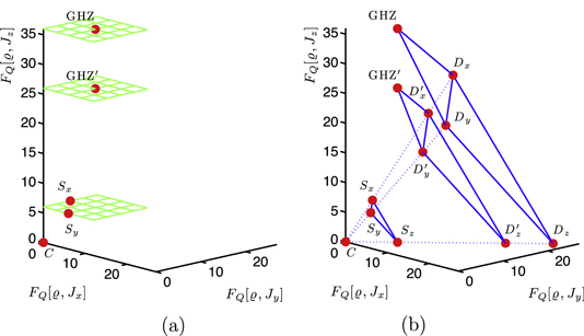
Figure 8. Entanglement criteria in the ![$({{F}_{Q}}[\varrho ,{{J}_{x}}],{{F}_{Q}}[\varrho ,{{J}_{y}}],{{F}_{Q}}[\varrho ,{{J}_{z}}])$](https://content.cld.iop.org/journals/1751-8121/47/42/424006/revision1/jpa500438ieqn213.gif) —space for N = 6 qubits. (a) Entanglement criteria with
—space for N = 6 qubits. (a) Entanglement criteria with ![${{F}_{Q}}[\varrho ,{{J}_{z}}].$](https://content.cld.iop.org/journals/1751-8121/47/42/424006/revision1/jpa500438ieqn214.gif) The planes correspond to the inequalities, from bottom to top, equation (100), (118a) and (101) with
The planes correspond to the inequalities, from bottom to top, equation (100), (118a) and (101) with  (b) Entanglement criteria with
 ![${{\sum }_{l}}{{F}_{Q}}[\varrho ,{{J}_{l}}].$](https://content.cld.iop.org/journals/1751-8121/47/42/424006/revision1/jpa500438ieqn216.gif) The planes correspond to the inequalities, from bottom to top, equation (108), (118b) and (109), respectively. For the description of the inequalities and the points see text.
The planes correspond to the inequalities, from bottom to top, equation (108), (118b) and (109), respectively. For the description of the inequalities and the points see text.
Download figure:
Standard image High-resolution imageIn figure 8(a), the entanglement conditions given in terms of an inequality with the quantum Fisher information ![${{F}_{Q}}[\varrho ,{{J}_{z}}]$](https://content.cld.iop.org/journals/1751-8121/47/42/424006/revision1/jpa500438ieqn217.gif) are shown. The completely mixed state corresponds to the point C at the origin. The entanglement criterion (100) corresponds to the bottom plane. Any state above this plane is entangled. For even
are shown. The completely mixed state corresponds to the point C at the origin. The entanglement criterion (100) corresponds to the bottom plane. Any state above this plane is entangled. For even  product states corresponding to the Sl points are defined as

for  The entanglement criterion (118a) corresponds to the second plane. Any state above this plane is genuine multipartite entangled. The point GHZ' refers to the state

Finally, the inequality (101) corresponds to the top plane. The point GHZ in figure 8(a) refers to the GHZ state given in (25).
Let us now turn to figure 8(b), in which the entanglement conditions involving the average quantum Fisher information (107) are shown. The plane of the triangle  corresponds to the inequality (108), all states above this plane are entangled. States corresponding to the points Sl are given in (119). The
 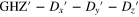 plane corresponds to the inequality (118b), and all states above this plane are genuine multipartite entangled. A tensor product of a Dicke state and a single-particle state corresponds to the point
where we used the definition of the symmetric Dicke state given in (33). Note that since  is odd,
  has unequal number of 0ʼs and 1ʼs. The points
  and
and  are defined similarly with Dicke states in the x and y-basis, respectively. The
  plane corresponds to (109). There are no physical states above this plane. The Dicke state in the z-basis characterized by (111) corresponds to the point
  The Dicke states in the x and y-basis correspond to the points Dx and
  respectively. GHZ states given in the x and y-basis, not shown in the figure 8(b), would also be in the same plane.
5.3. Macroscopic superposition
After describing the relation between the quantum Fisher information and multiparticle entanglement, we will discuss one of the related interesting questions, namely, the proper definition of a macroscopic superposition [123–125]. The question whether a quantum state is a macroscopic superposition makes sense only if we consider a state that can be defined for any number of particles, such as the GHZ state. Then, we examine the properties of this family of states for an increasing 
A very meaningful definition has been proposed for pure states based on the variance of collective quantities as follows [123]. Let us define  as the set of collective operators given as
Here  are single-particle operators acting on the
  particle and for the operator norm we require
  Note that before A was just a general Hermitian operator, however, from now on we require that it is the sum of single-particle operators. For spin-
 particles and traceless
  the operators of the type (122) are just the collective angular momentum component Jz apart from local unitaries and a constant factor.
Then, we can define the index p as

Here,  means that
  The index p in (123) is confined in a range
  and for any product state we have
  The state is called macroscopically entangled if p = 2. These ideas can be extended to mixed states using the quantum Fisher information rather than the variance [124, 125]. The effective size of a macroscopic superposition is defined as

We call a quantum state a macroscopic superposition if 
We can compare this definition to our findings concerning the relationship between multipartite entanglement and the quantum Fisher information in section 5.2. Based on (116), we can see that for N divisible by  for k-producible states we have
  Hence, for a quantum state to be a macroscopic superposition, it is necessary that the state is k-particle entangled such that
  Thus, k must grow linearly with
  while we do not need to have full N-body entanglement.
Since the quantum Fisher information is convex, as discussed in section 4.2, if we mix two states with each other that are not macroscopic quantum superpositions, we will always get a state that is not a macroscopic quantum superposition either. Hence, states that are not macroscopic quantum superpositions form a convex set. This is, of course, expected for a meaningful definition. Moreover, since the quantum Fisher information is the convex roof of the variance, as discussed in section 4.2, it is always larger or equal to other convex functions that for pure states equal four times the variance. Hence our definition gives a larger set of states forming a macroscopic superpositions than if we used instead of the quantum Fisher information (59) generalized quantum Fisher informations, like four times the Wigner–Yanase skew information (65) mentioned earlier.
5.4. Speed of quantum evolution
In this section, we discuss that the entanglement properties of a quantum state are related to the speed of the quantum evolution starting out from the state, via the quantum Fisher information [126, 127]. We will show that states with a large quantum Fisher information, and thus, a large multiparticle entanglement can evolve faster than states with a small quantum Fisher information.
We use the Bures fidelity to describe the speed of the evolution. This quantity plays a central role in quantum information science. It is defined as

Clearly,  The fidelity is 1 only if
  while it is 0 if the two states live in orthogonal subspaces. If ϱ1 is a pure state, then the fidelity can be expressed in a simpler form

If both states are pure, then the fidelity is just the square of the absolute value of the overlap

The fidelity can be used to characterize the speed of the evolution by calculating the fidelity between the initial state ϱ and the final state  Using the fact that the quantum Fisher information is proportional to the second derivative of the fidelity with respect to
  in this case, we can write [126, 127]

where the parameter θ is small and the system Hamiltonian is given by  Note that there cannot be a term linear in θ since such a term would result in
  either for
  or for
  for small
  Apart from the expansion (128), a bound for the fidelity can be obtained from the improved Madelstam–Tamm bound [128]

with the condition

Based on the properties of the fidelity described above, we can interpret the relation (128) in the following way. As θ is increasing, the fidelity with respect to the initial state starts to decrease. The quantum Fisher information ![${{F}_{Q}}[\varrho ,A]$](https://content.cld.iop.org/journals/1751-8121/47/42/424006/revision1/jpa500438ieqn255.gif) in (128) characterizes the speed at which the quantum state evolves into a state orthogonal to the initial state.
in (128) characterizes the speed at which the quantum state evolves into a state orthogonal to the initial state.
If A is the sum of single-particle operators, i.e.,  then the speed of the evolution is related to the entanglement of the quantum state. One can see that large quantum Fisher information is needed for a large speed. Based on section 5.2, it is also clear that for a large quantum Fisher information a large multipartite entanglement is needed. Thus, large multiparticle entanglement is needed for a large speed of the quantum evolution.
5.5. Quantum Zeno effect
The quantum Zeno effect is one of the most discussed paradoxical features of quantum mechanics. It has been recently shown that it is related to the quantum Fisher information. Due to the Zeno effect, if we have a quantum system in an initial state, that starts to evolve under a Hamiltonian, and we perform a projective measurement, projecting the state to the initial state, with a sufficient frequency then the system will be unable to evolve, and stays in the initial state. This can be expressed more quantitatively as follows. If we perform m measurements at times  for
for  such that
 and
and  then we find that the quantum system does not evolve and it stays in its initial state. It turns out that the characteristic quantum Zeno time is [129, 130]

In order to see the quantum Zeno effect, we need to perform the projective measurements with a frequency larger than 
As in the case of the speed of the quantum evolution, it is interesting to consider the case when A is the sum of single-particle operators. Then, based on (131), we see that for states with a large quantum Fisher information  is small. Hence, based on section 5.2, for entangled states
  can be
  while for separable states we obtain
  These show that the entanglement properties of a quantum state are reflected in its behaviour in the quantum Zeno effect.
5.6. Multi-particle entanglement versus mode-entanglement
In this section, we discuss the meaning of multipartite entanglement of very many particles. The full discussion of this topic is outside of the scope of our review. However, we would mention connections of this problem to the topics covered here.
Entanglement is typically considered between two- or more parties that are spatially separated from each other and are individually accessible. This is due to the fact that entanglement theory developed from the theory of Bell inequalities that required even a space-like separation of the detection events at the parties [23, 24]. Moreover, distillation of entanglement by local operations and classical communication, and many other quantum information processing tasks need a local access to the particles [23, 24].
However, in a many-particle system, where we have  particles, this picture cannot be maintained, since even with a large technological advancement we would not be able to access the particles individually. The situation is even more complicated when we consider Bose–Einstein condensates of two-state atoms. In this case, ideally, all the atoms occupy the same spatial state.
Internal quantum states of Bose–Einstein condensates of two-state atoms can be written as an N-qubit symmetric quantum state or as a two-mode quantum state. The two descriptions are equivalent to each other. For example, the GHZ state as a multiparticle state is given in (25), while as a two-mode state can be given in (31). It can happen that a state that is highly entangled in one description is not entangled in the other, and vice versa. It has been argued by some authors that for states of Bose–Einstein condensates, the entanglement between the modes has to be considered rather than entanglement between particles [131, 132]. It has been shown that the precision can surpass the shot-noise limit in a linear interferometer with non-entangled states, i.e., states without entanglement between the modes [131].
The previous sections of this review help us to analyse this question from the point of view of quantum metrology. As discussed in section 5.1, inter-particle entanglement is needed to overcome the shot-noise limit for linear interferometers. The entanglement condition based on metrological usefulness is equally valid for ensembles of individually accessible particles and ensembles of particles that are not accessible individually. In fact, it is also valid for quantum states of Bose–Einstein condensates. If the state satisfies the definition of separability (43) then it cannot surpass the shot-noise limit, even in a Bose–Einstein condensate. The same is true for multiparticle entanglement, as discussed in section 5.2. Full multiparticle entanglement is needed to reach the maximum precision. Moreover, the definition of macroscopic superposition given in section 5.3 does not require individually accessible particles. Finally, this is also true for our findings relating the quantum Fisher information to the speed of evolution discussed in section 5.4. There is a maximal speed for separable multi-particle states satisfying (43), regardless of whether the particles can be individually accessed or not. Based on these, it seems to be reasonable to say that inter-particle entanglement is a very useful notion even for large ensembles and even for a Bose–Einstein condensate of two-state atoms.
Still, it remains an important question whether the interparticle entanglement within Bose–Einstein condensates can be converted into entanglement between individually accessible particles. An insight concerning this question can be gained from the dilute cloud argument [105]. This thought-experiment, shown in figure 9, demonstrates that an ensemble of two-state particles in a Bose–Einstein condensate can be converted to an ensemble of localized particles, while the internal state of the ensemble remains unchanged. Finally, entanglement within a Bose–Einstein condensate of two-state atoms can be converted to entanglement between two spatial modes of the same particles with straightforward non-entangling operations [133]. This statement can even be generalized to the case of splitting the condensate into three or more ensembles entangled with each other.
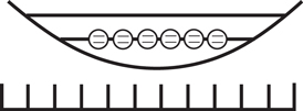
Figure 9. The dilute cloud argument. While in the Bose–Einstein condensate, the two-state particles occupy the same spatial mode. If we let the cloud expand, and we detect the particle positions with detectors that do not disturb the internal state of the atoms, we obtain an ensemble of distinguishable particles with the same internal state that they had in the Bose–Einstein condensate. If we have much more detectors than particles in a dilute cloud, we can achieve that no two particles end up at the same detector.
Download figure:
Standard image High-resolution image
6. Metrology in a noisy environment
In this section, we examine what happens if noise appears in the quantum metrological setup. We will show that uncorrelated noise can easily destroy the Heisenberg scaling (2) and restore the shot-noise scaling (1), above a certain particle number.
In order to gain an intuitive understanding, let us consider the example of magnetometry with spin squeezed states discussed in section 2.1 and examine the effect of uncorrelated noise. Let us assume that a particle with a state ϱ1 passes trough a map that turns its internal state to the fully mixed state with some probability p as

If this map acts in parallel on all particles, the state can be given as a mixture

where the state obtained after n particles decohered into the completely mixed state is

Here the summation is over all permutations Πk, since we took advantage of the fact that the spin squeezed state is permutationally invariant. This is a reasonable assumption, as both the initial state and the spin squeezing dynamics are typically permutationally invariant. The quantity pn in the decomposition (133) is obtained with the binomial coefficients as

For the noisy state (133), the variance of the collective angular momentum component can be bounded from below as

For the first inequality in (136), we used the concavity of the variance. For the second inequality, we used the fact that for a product state of the form  the variance is the sum of the variances for ϱk

Note that  and
and  are possibly multi-particle states. To obtain the bound on the right-hand side of (136), we used a well-known identity for the binomial coefficients

where pn is defined in (135). The equality (138) expresses the fact that the expectation value of the number of spins that undergo decoherence is  In the bound on the variance (136) the term linear in N appears since, in average, the same fraction of the spins is affected for all N and all the decohered spins introduce the same additional noise for the collective angular momentum component. Based on these and on the formula (14) giving the precision, we obtain
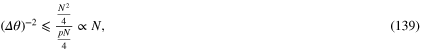
which means that the precision has a shot-noise scaling for large  It is important to note that this is true whenever
  hence any nonzero decoherence will lead to a shot-noise scaling.
After this instructive example, let us review the existing literature on the subject. The effect of the noise has been analysed for a setup based on metrology with GHZ states described in section 2.2. Let us consider the dynamics

where the first term describes the coherent evolution, while the second term is the decoherence. The single-particle decoherence is given as

where  is the overall noise strength, ϱ1 is a single-particle state, σl are the Pauli spin matrices,
  and
and  In [134], it has been shown that for
  the GHZ state does not provide a better scaling of the precision with the particle number than uncorrelated states. On the other hand, states leading to an optimal precision are different from the GHZ state.
Recently, it has been proven in a very general framework that in the presence of even very small decoherence,  scales with N rather than with N2 for large particle numbers [59, 108, 135]. Let us consider the single-particle map

where Ek are the usual POVM elements. Let us assume that this map acts on the input state on all particles independently, and we use the state obtained from this map to estimate the parameter  Thus, while before we estimated the parameter in a unitary evolution, now we need to estimate the parameter of the incoherent dynamics. The corresponding quantum Fisher information will be denoted by
 ![${{F}_{Q}}[\Lambda _{\theta }^{\otimes N}[\varrho ]].$](https://content.cld.iop.org/journals/1751-8121/47/42/424006/revision1/jpa500438ieqn280.gif)
According to reference [135], the quantum Fisher information for this incoherent evolution can be computed as

On the right-hand side, there is a minimization carried out over all the purifications of the dynamics  for which

where  means tracing out the environment and the extended system consists of the original system and the environment. The minimization in (143) is analogous to the infimum in the convex roof construction of (64). If we find a purification which is not the optimal one, based on (143), it will still give an upper bound on the quantum Fisher information, which can be used to prove the shot-noise scaling of particular quantum metrological setups.
Reference [108] presented an alternative proof based on the classical simulation of channels. Let us assume that a single-particle channel is obtained as a mixture of other channels as

Then, the Cramér–Rao bound gives a lower bound on the variance of the parameter to be estimated as
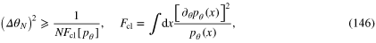
where  is the classical Fisher information. Note that
  characterizes the single-particle channel, thus it does not depend on
  Thus, if
  then we obtain
  which means a shot-noise scaling for large
  It can be shown that
  for all channels that are not θ-extremal. The behaviour of such channels for small θ can always be described by the mixture of two channels that are at the boundary of the set of channels. A third proof in [108], working also for θ-extremal channels, makes it possible to avoid the optimization over purifications by carrying out the optimization in an extended system.
Reference [136] presents a general formalism for open system metrology, which is able handle complicated non-unitary dynamics and provides a lower and an upper bound for the quantum Fisher information. In general, there has been a large recent interest in parameter estimation in non-unitary processes, however, this topic is outside of the scope of the review (e.g., see [119, 137]).
Due the uncorrelated noise, the states obtained can efficiently be described by matrix product states [138]. The change of the scaling of the precision to a shot-noise scaling for large N has been observed also in the analysis of the scaling for the squeezed-light-enhanced gravitational wave detector GEO 600 [139].
There have been several attempts to beat the shot-noise scaling in the large particle number limit even in the light of the above results. For example, in metrology with GHZ states described in section 2.2, [140] considers a frequency measurement such that there is an optimization over the duration of the dynamics. Hence, the single-particle channel depends on  while it was independent of N in the discussion above. It is shown that the shot-noise limit can be surpassed for a particular type of dephasing, concretely, for the
  case in the decoherence model given in (141). Note, however, that the shot-noise scaling is restored for large N whenever
  e.g., if
  Moreover, very recently, quantum error correction has been used in proposals to reach a Heisenberg scaling in a noisy environment [141, 142].
So far we have been discussing metrological setups for an ensemble of particles that do not interact with each other. Such setups play an important role in metrology, as it is much easier to create dynamics with non-interacting particles in a controlled manner, than dynamics based on two-body interactions. With interactions, the precision can surpass the shot-limit of the non-interacting case even starting from a product state, or it can surpass the Heisenberg limit of the non-interacting case [25–31]. It is instructive to obtain the maximal scaling for systems with q-body interactions as follows. Let us take the Hamiltonian  For this Hamiltonian,
 ![${{F}_{Q}}[\varrho ,{{H}_{q}}]/4\leqslant {{(\Delta {{H}_{q}})}^{2}}\leqslant {{(\frac{N}{2})}^{2q}}=\mathcal{O}({{N}^{2q}}).$](https://content.cld.iop.org/journals/1751-8121/47/42/424006/revision1/jpa500438ieqn295.gif) Similar derivation works also for any Hamiltonian with at most q-particle interactions. However, for a wide class of noise models, uncorrelated noise affects these setups in way analogous to the linear case: due to the uncorrelated noise, only
Similar derivation works also for any Hamiltonian with at most q-particle interactions. However, for a wide class of noise models, uncorrelated noise affects these setups in way analogous to the linear case: due to the uncorrelated noise, only  can be reached for large N [143].
All the statements above are for uncorrelated noise. The case of correlated noise has also been studied intensively (e.g., see [144–147]). For certain types of correlated noise, the Heisenberg scaling can be reached.
Finally, it is important to recognize that our observations concerning the effect of the noise in quantum metrology are connected to fundamental questions in quantum physics. In section 5.2, we have shown that for a large metrological precision a large entanglement depth is also needed. Naturally arises the question whether it is possible to reach a large entanglement depth, especially for large particle numbers in a noisy environment. Hence, quantum metrology is connected to several other fields examining the survival of large scale entanglement in a noisy environment [138]. For example, a related topic is the physics of nanosystems at a finite temperature [148, 149]. For such systems, the density matrix of a system is very close to a tensor product of density matrices of subsystems. The larger the temperature, the smaller the size of the terms can be. This is connected to the fact that multipartite entanglement cannot survive easily at finite temperatures.
7. Conclusions
We have discussed the basics of quantum metrology through simple examples of metrology with a fully polarized ensemble of particles or with highly entangled states. After this introduction, we presented the basic formalism of quantum metrology based on the quantum Fisher information and the Cramér–Rao bound. We discussed that for dynamics with a Hamiltonian that does not contain interaction terms, the usefulness of quantum states for metrology is closely related to their entanglement properties. We found that separable states can achieve only a shot-noise scaling, while for states with high level of entanglement even the Heisenberg scaling is possible. Finally, we discussed how uncorrelated noise can affect this situation, leading back to a shot-noise scaling for large particle numbers even for entangled states.
Acknowledgments
We thank S Altenburg, E Bagan, N Behbood, J Calsamiglia, G Colangelo, M Cramer, R Demkowicz-Dobrzański, F Deuretzbacher, B Escher, IL Equsquiza, F Fröwis, O Gühne, P Hyllus, M Kleinmann, C Klempt, B Kraus, B Lücke, MW Mitchell, M Modugno, A Monras, M Oberthaler, D Petz, L Pezzé L Santos, C Schwemmer, RJ Sewell, A Smerzi, R Schmied, and H Weinfurter for interesting discussions. We thank O Gühne for calling our attention to the entanglement of assistance measures for section 4.2, and P Hyllus for discussions about entanglement in systems of very many particles connected to section 5.6. A special thank to the members of the group funded by the ERC StG GEDENTQOPT at the University of the Basque Country UPV/EHU, to I Urizar-Lanz, G Vitagliano, and Z Zimborás for discussions. Finally, we would like to thank the participants of the conference on Entanglement Detection and Quantificaton held in Bilbao in 2014 for many valuable discussions. We acknowledge the support of the EU (ERC Starting Grant GEDENTQOPT, CHIST-ERA QUASAR) the Spanish MINECO (Project No. FIS2009-12773-C02-02 and No. FIS2012-36673-C03-03), the Basque Government (Project No. IT4720-10), and the National Research Fund of Hungary OTKA (Contract No. K83858).
Footnotes
- 4
The fact that the second inequality of (67) can be saturated means that there is a decomposition such that the average variance of the pure states of the decomposition equals the variance of the mixed state. It is possible to prove an analogous statement for 2 × 2 covariance matrices, while this is not always true for 3 × 3 covariance matrices [98, 99].