

Abstract
One of the most widely known building blocks of modern physics is Heisenberg's indeterminacy principle. Among the different statements of this fundamental property of the full quantum mechanical nature of physical reality, the uncertainty relation for energy and time has a special place. Its interpretation and its consequences have inspired continued research efforts for almost a century. In its modern formulation, the uncertainty relation is understood as setting a fundamental bound on how fast any quantum system can evolve. In this topical review we describe important milestones, such as the Mandelstam–Tamm and the Margolus–Levitin bounds on the quantum speed limit, and summarise recent applications in a variety of current research fields—including quantum information theory, quantum computing, and quantum thermodynamics amongst several others. To bring order and to provide an access point into the many different notions and concepts, we have grouped the various approaches into the minimal time approach and the geometric approach, where the former relies on quantum control theory, and the latter arises from measuring the distinguishability of quantum states. Due to the volume of the literature, this topical review can only present a snapshot of the current state-of-the-art and can never be fully comprehensive. Therefore, we highlight but a few works hoping that our selection can serve as a representative starting point for the interested reader.
Export citation and abstract BibTeX RIS
1. Introduction
It is a historic fact that Einstein never seemed quite comfortable with the probabilistic interpretation of quantum theory. In a letter to Born he once remarked [1]:
Quantum mechanics is certainly imposing. But an inner voice tells me that it is not yet the real thing. The theory says a lot, but does not really bring us any closer to the secret of the old one. I, at any rate, am convinced that He does not throw dice3.
Nevertheless, quantum mechanics is built on the very notion of indeterminacy, which is rooted in Heisenberg's uncertainty principles, and which can be expressed in terms of the famous inequalities [2, 3],

Although physically insightful, these relations, equation (1), were originally motivated only by plausibility arguments and by 'observing' the commutation relations of canonical variables in first quantization4.
While the uncertainty relation for position and momentum was quickly put on solid grounds by Bohr [4] and Robertson [5], the proper formulation and interpretation for the uncertainty relation of time and energy proved to be a significantly harder task. In its modern interpretation the uncertainty relation for position and momentum expresses the fact that the position and the momentum of a quantum particle cannot be measured simultaneously with infinite precision [6]. However, if the uncertainty principle is a statement about simultaneous events, the interpretation of an uncertainty in time is far from obvious [7].
Thus, only three years after its inception Einstein challenged the validity of the energy-time uncertainty relation with the following gedankenexperiment as depicted in figure 1 [8]: Imagine a box containing photons, which has a hole in one of its walls. This hole can be opened and closed by a shutter controlled by a clock inside the box. At a preset time the shutter opens the hole for a short period and lets photons escape. Since the clock can be classical, the duration can be determined with infinite precision. From special relativity we know that energy and mass are equivalent,  . Hence, by measuring the mass of the box in the gravitational field, the change in energy due to the loss of photons can also be determined with infinite precision. As a consequence, special relativity seems to negate the existence of an uncertainty principle for energy and time!

Figure 1. Sketch of the gedankenexperiment envisaged by Einstein. Figure courtesy of Marta Paczyńska.
Download figure:
Standard image High-resolution imageBohr's counterargument in essence states that in order to measure time, position and momentum of the hands of the clock have to be determined. In addition, accounting for time dilation due to motion in the gravitational field, the uncertainty relation for position and momentum implies an uncertainty relation for energy and time. Although insightful, Bohr's interpretation cannot be considered entirely satisfactory [7–9], since it merely circumvents the problem of explaining the existence of the uncertainty principle in non-relativistic quantum mechanics.
A major breakthrough was achieved by Mandelstam and Tamm [10], who realised that  is not a statement about simultaneous measurements, but rather about the intrinsic time scale of unitary quantum dynamics. Hence, one should rather write
  , where
  is interpreted as the time a quantum system needs to evolve from an initial to a final state. More specifically Mandelstam and Tamm derived the first expression of the quantum speed limit time
 ![$ \newcommand{\mrm}[1]{{\rm #1}} \tau_\mrm{QSL}=\pi\hbar/2\Delta H$](https://content.cld.iop.org/journals/1751-8121/50/45/453001/revision2/aaa86c6ieqn006.gif) , where
, where  is the variance of the Hamiltonian, H, of the quantum system [10]. As an application of their bound, they also argued that
 ![$ \newcommand{\mrm}[1]{{\rm #1}} \tau_\mrm{QSL}$](https://content.cld.iop.org/journals/1751-8121/50/45/453001/revision2/aaa86c6ieqn008.gif) naturally quantifies the life time of quantum states [10], which has found widespread prominence in the literature [11–16].
naturally quantifies the life time of quantum states [10], which has found widespread prominence in the literature [11–16].
Nevertheless, the desire to formalise time as a proper quantum observable persisted [17, 18]. To make matters worse, it was further argued that the variance of an operator is not an adequate measure of quantum uncertainty [19, 20], which only highlighted that the uncertainty relation for time and energy needed to be put on even firmer grounds.
With the advent of quantum computing [21, 22] Mandelstam and Tamm's interpretation of the quantum speed limit as intrinsic time-scale experienced renewed prominence. Their interpretation was further solidified by Margolus and Levitin [23], who derived an alternative expression for ![$ \newcommand{\mrm}[1]{{\rm #1}} \tau_\mrm{QSL}$](https://content.cld.iop.org/journals/1751-8121/50/45/453001/revision2/aaa86c6ieqn009.gif) in terms of the (positive) expectation value of the Hamiltonian,
in terms of the (positive) expectation value of the Hamiltonian, ![$ \newcommand{\la}{\left\langle} \newcommand{\ra}{\right\rangle} \newcommand{\mrm}[1]{{\rm #1}} \tau_\mrm{QSL}=\pi\hbar/2 \la H\ra$](https://content.cld.iop.org/journals/1751-8121/50/45/453001/revision2/aaa86c6ieqn010.gif) . Eventually, it was also shown that the combined bound,
. Eventually, it was also shown that the combined bound,

is tight [24]. This means equation (2) sets the fastest attainable time-scale over which a quantum system can evolve. In particular, equation (2) sets the maximal rate with which quantum information can be communicated [25], the maximal rate with which quantum information can be processed [26], the maximal rate of quantum entropy production [27], the shortest time-scale for quantum optimal control algorithms to converge [28], the best precision in quantum metrology [29], and determines the spectral form factor [30].
The next major milestone in the development of the field was achieved only relatively recently with the generalisation of the quantum speed limit to open systems. In 2013 three letters proposed, in quick succession, three independent approaches of how to quantify the maximal quantum speed of systems interacting with their environments. Taddei et al [31] found an expression in terms of the quantum Fisher information, del Campo et al [32] bounded the rate of change of the relative purity, and Deffner and Lutz [33] derived geometric generalizations of both, the Mandelstamm–Tamm bound as well as the Margolus–Levitin bound. These three contributions [31–33] effectively opened a new field of modern research, since for the first time it became obvious that the Heisenberg uncertainty principle for time and energy is not only of fundamental importance, but actually of quite practical relevance. For instance, it became clear that quantum processes in systems interacting with non-Markovian environments can evolve faster than in systems coupled to memory-less, Markovian baths—which has been verified in a cavity QED experiment [34].
The purpose of this topical review is to take a step back and bring order into the plethora of novel ideas, concepts, and applications. Thus, in contrast to earlier reviews on quantum speed limits [35–42], we will focus less on mathematical and technical details, but rather emphasise the interplay between the various concepts, tradeoffs between speed and physical resources, and consequences in real-life applications. We will begin with a historical overview in section 2, where we will also summarise the original derivations by Mandelstam–Tamm and Margolus–Levitin. Section 3 is dedicated to quantum systems with time-independent generators, whereas section 4 focuses on optimal control theory. In section 5 we will discuss the geometric approach, which so far has been the most fruitful approach in the description of open quantum systems, and which has led to the most interesting insights. The review is rounded off with section 6, in which we briefly summarise generalisations to relativistic and non-linear quantum dynamics, and section 7 which outlines the relation of quantum speed limits to other fundamental bounds.
When writing this topical review, we strove for objectivity and completeness. However, the sheer volume of publications demanded to select but a few works to be discussed in detail. Our selection was motivated by accessibility, pedagogical value, and conceptual milestones. Therefore, this review can never be a fully complete discussion of the literature, but rather only serve as a starting point for further study and research on quantum speed limits.
2. Energy-time uncertainty: emergence of the quantum speed limit
2.1. Heisenberg's uncertainty principle
For classical observers, one of the most remarkable properties of quantum systems is the inherent indeterminism of physical states that have not been measured. This indeterminism originates from trying to resolve the apparent wave-particle duality, which necessitates a probabilistic theory to describe the behaviour of small objects [2, 3]. The most prominent hallmark of this insight is the indeterminacy principle, which is typically expressed as the uncertainly relation,

This relation reflects that the position and momentum of a quantum particle cannot be measured simultaneously with infinite precision5.
In introductory texts equation (3) is often motivated by analysing the Fourier modes of wave packets [43], which then also allows to derive an additional uncertainty relation for time, t, and energy, E. To this end, one identifies [43]

where v denotes the group velocity of a wave packet. Therefore, one concludes

which now expresses that also time and energy cannot be known simultaneously with infinite precision.
That something of this argumentation is a bit fishy [7, 8] becomes clear once one realises that the uncertainty principle for position and momentum is actually a consequence of the canonical commutation relation,

It was shown by Roberston [5] by simply invoking the Cauchy–Schwarz inequality [43] that for any two operators A and B we have

where  with
with  and
and ![$ \renewcommand{\bra}[1]{\left\langle #1\right\vert} \renewcommand{\ket}[1]{\left\vert #1\right\rangle} \newcommand{\la}{\left\langle} \newcommand{\ra}{\right\rangle} \la O\ra=\bra{\psi}O\ket{\psi}$](https://content.cld.iop.org/journals/1751-8121/50/45/453001/revision2/aaa86c6ieqn013.gif) . Strictly speaking (7) does not correspond to simultaneous measurements since the quantum back action of measurements is not considered [44], and see also section 7.4. Rather, equation (7) can be understood as a special case of the Cramer–Rao bound [45, 46], and thus the uncertainty relation must be interpreted as a statement about the preparation of states, see also sections 3.4 and 7.1. Imagine that an observable A is measured on the first half of an ensemble, and B on the second half, then equation (7) sets a limit on the product of standard deviations.
. Strictly speaking (7) does not correspond to simultaneous measurements since the quantum back action of measurements is not considered [44], and see also section 7.4. Rather, equation (7) can be understood as a special case of the Cramer–Rao bound [45, 46], and thus the uncertainty relation must be interpreted as a statement about the preparation of states, see also sections 3.4 and 7.1. Imagine that an observable A is measured on the first half of an ensemble, and B on the second half, then equation (7) sets a limit on the product of standard deviations.
Independent of the interpretation of equation (7) time can, generally, not be expressed as a Hermitian operator [7–9, 47], and hence equation (7) cannot be reduced to the Heisenberg energy-time uncertainty relation (5). To avoid any misconceptions we emphasize that other time-like variables such as arrival or tunneling times [38, 39] can very well be expressed as operators.
In this topical review, 'time' will always be understood as the quantity with which one commonly associates an uncertainty relation of the form (5). From its first appearance of such a notion of time in Heisenberg's paper in 1927 [2] it took almost twenty years before a mathematically sound and physically insightful treatment was proposed by Mandelstam and Tamm [10].
2.2. The uncertainty relation of Mandelstam and Tamm
Mandelstam and Tamm's analysis [10] rests on the fact that for quantum systems evolving under Schrödinger dynamics the evolution of any observable A is given by the Liouville-von-Neumann equation

where H is the Hamiltonian of the system. Therefore, the general uncertainty relation in equation (7) implies for 

The latter inequality can be further simplified, if we choose the observable A as the projector onto the initial state ![$ \newcommand{\ra}{\right\rangle} \renewcommand{\ket}[1]{\left\vert #1\right\rangle} \ket{\psi(0)}$](https://content.cld.iop.org/journals/1751-8121/50/45/453001/revision2/aaa86c6ieqn015.gif) , and
, and ![$ \newcommand{\la}{\left\langle} \renewcommand{\bra}[1]{\left\langle #1\right\vert} \newcommand{\ra}{\right\rangle} \renewcommand{\ket}[1]{\left\vert #1\right\rangle} A=\ket{\psi(0)}\bra{\psi(0)}$](https://content.cld.iop.org/journals/1751-8121/50/45/453001/revision2/aaa86c6ieqn016.gif) . Thus, we also have
. Thus, we also have  and
and

which allows to integrate equation (9) and we obtain,

If we now consider only processes in which the final state is orthogonal to the initial state, i.e. ![$ \renewcommand{\bra}[1]{\left\langle #1\right\vert} \newcommand{\la}{\left\langle} \newcommand{\ra}{\right\rangle} \renewcommand{\braket}[2]{\left\langle #1\vert #2\right\rangle} \braket{\psi(0)}{\psi(\tau)}=0$](https://content.cld.iop.org/journals/1751-8121/50/45/453001/revision2/aaa86c6ieqn018.gif) , then the minimal time for a quantum system to evolve between two orthogonal states is determined by
, then the minimal time for a quantum system to evolve between two orthogonal states is determined by

As a main breakthrough, Mandelstam and Tamm not only put Heisenberg's uncertainty principle for time and energy on solid physical grounds, but also proposed the first notion of a quantum speed limit time, ![$ \newcommand{\mrm}[1]{{\rm #1}} \tau_\mrm{QSL}$](https://content.cld.iop.org/journals/1751-8121/50/45/453001/revision2/aaa86c6ieqn019.gif) (12). It is interesting to note that the proper interpretation of the energy-time uncertainty principle as a bound on the minimal time of quantum evolution was formalised by Aharonov and Bohm [48]. They pointed out that equation (12) must not be interpreted as an uncertainty relation between the duration of a measurement and the energy transferred to the observed system. Rather, the quantum speed limit time,
(12). It is interesting to note that the proper interpretation of the energy-time uncertainty principle as a bound on the minimal time of quantum evolution was formalised by Aharonov and Bohm [48]. They pointed out that equation (12) must not be interpreted as an uncertainty relation between the duration of a measurement and the energy transferred to the observed system. Rather, the quantum speed limit time, ![$ \newcommand{\mrm}[1]{{\rm #1}} \tau_\mrm{QSL}$](https://content.cld.iop.org/journals/1751-8121/50/45/453001/revision2/aaa86c6ieqn020.gif) , sets an intrinsic time scale of any quantum evolution [48, 49].
, sets an intrinsic time scale of any quantum evolution [48, 49].
Over the next four decades ![$ \newcommand{\mrm}[1]{{\rm #1}} \tau_\mrm{QSL}$](https://content.cld.iop.org/journals/1751-8121/50/45/453001/revision2/aaa86c6ieqn021.gif) (12) was frequently studied and re-derived by Fleming [50], Bhattacharyya [51], Anandan and Aharonov [52], and Vaidman [53]. However, it was Uffink who realised [19] that in many situations
(12) was frequently studied and re-derived by Fleming [50], Bhattacharyya [51], Anandan and Aharonov [52], and Vaidman [53]. However, it was Uffink who realised [19] that in many situations  gives a very unreasonable measure for the speed of a quantum evolution. The lower bound in equation (12) can be arbitrarily small, since the variance of the Hamiltonian,
  , can diverge even if the average energy is finite [23].
2.3. The quantum speed limit of Margolus and Levitin
To tackle this problem Margolus and Levitin proposed an alternative derivation of the quantum speed limit [23]. Their analysis starts with expanding the initial state, ![$ \newcommand{\ra}{\right\rangle} \renewcommand{\ket}[1]{\left\vert #1\right\rangle} \ket{\psi_0}$](https://content.cld.iop.org/journals/1751-8121/50/45/453001/revision2/aaa86c6ieqn024.gif) , in the energy eigenbasis
, in the energy eigenbasis

Correspondingly, the solution to the time-dependent Schrödinger equation with constant Hamiltonian can be written as,

and we obtain for the time-dependent overlap with the initial state ![$ \renewcommand{\bra}[1]{\left\langle #1\right\vert} \newcommand{\la}{\left\langle} \newcommand{\ra}{\right\rangle} \renewcommand{\braket}[2]{\left\langle #1\vert #2\right\rangle} \newcommand{\ex}[1]{\exp{\left(#1\right)}} \newcommand{\e}{{\rm e}} S(t)\equiv \braket{\psi_0}{\psi_t}=$](https://content.cld.iop.org/journals/1751-8121/50/45/453001/revision2/aaa86c6ieqn025.gif)
![$ \renewcommand{\bra}[1]{\left\langle #1\right\vert} \newcommand{\la}{\left\langle} \newcommand{\ra}{\right\rangle} \renewcommand{\braket}[2]{\left\langle #1\vert #2\right\rangle} \newcommand{\ex}[1]{\exp{\left(#1\right)}} \newcommand{\e}{{\rm e}} \sum_n \left\vert c_n\right\vert ^2 \ex{-{\rm i}\, E_n t/\hbar}$](https://content.cld.iop.org/journals/1751-8121/50/45/453001/revision2/aaa86c6ieqn026.gif) . The quantum speed limit is then obtained by estimating the real part of
. The quantum speed limit is then obtained by estimating the real part of 

where we have used the trigonometric inequality, ![$ \newcommand{\co}[1]{\cos{\left(#1\right)}} \newcommand{\si}[1]{\sin{\left(#1\right)}} \co{x}\geqslant1-2/\pi\, (x+\si{x})$](https://content.cld.iop.org/journals/1751-8121/50/45/453001/revision2/aaa86c6ieqn028.gif) , which is true
, which is true  . Note that we here explicitly assume that the average energy,
  , is non-negative. Now, further noting that for orthogonal initial and final states we have
  , which also implies
 ![$ \newcommand{\ma}[1]{\max{\left\{#1\right\}}} \newcommand{\mf}[1]{\mathfrak{#1}} \mf{R}(S)=0$](https://content.cld.iop.org/journals/1751-8121/50/45/453001/revision2/aaa86c6ieqn032.gif) and
and ![$ \newcommand{\ma}[1]{\max{\left\{#1\right\}}} \newcommand{\mf}[1]{\mathfrak{#1}} \mf{I}(S)=0$](https://content.cld.iop.org/journals/1751-8121/50/45/453001/revision2/aaa86c6ieqn033.gif) , and we obtain the minimal evolution time between two orthogonal states,
, and we obtain the minimal evolution time between two orthogonal states,

The Margolus–Levitin bound, equation (16), does not suffer from the conceptual issues that plagued the Mandelstam–Tamm bound—namely that the dynamical speed is determined by the variance of some quantum observable [19]. However, the discovery of equation (16) also created the paradoxical situation that there seem to exist two apparently independent bounds based on two different physical properties of the same quantum state [24]. That both bounds, (12) and (16), hold true, however, was illustrated by further elementary proofs by, e.g. Uffink [19], Brody [54], Andrecut and Ali [55], and Kosiński and Zych [56], and by more eleborated proofs for mixed and entangled states [57–59].
2.4. The unified bound is tight
As a consequence it was simply assumed without much justification that the minimal time a quantum system needs to evolve between two orthogonal states is given by

However, it was Levitin and Toffoli [24], who finally realised that the situation is not quite that simple. To this end, they proved the following theorem:
Under the assumption that the ground state energy of a quantum systems is zero, the only state for which the Mandelstam–Tamm bound equation (12) as well as the Margolus–Levitin bound equation (13) are attained is given by
where
for all

![$ \newcommand{\ra}{\right\rangle} \renewcommand{\ket}[1]{\left\vert #1\right\rangle} H\ket{E_k}=k E_1\, \ket{E_k}$](https://content.cld.iop.org/journals/1751-8121/50/45/453001/revision2/aaa86c6ieqn034.gif)

![$ \newcommand{\ra}{\right\rangle} \renewcommand{\ket}[1]{\left\vert #1\right\rangle} \ket{\psi}$](https://content.cld.iop.org/journals/1751-8121/50/45/453001/revision2/aaa86c6ieqn036.gif)
2.4.1. Margolus–Levitin bound.
That ![$ \newcommand{\ra}{\right\rangle} \renewcommand{\ket}[1]{\left\vert #1\right\rangle} \ket{\psi}$](https://content.cld.iop.org/journals/1751-8121/50/45/453001/revision2/aaa86c6ieqn037.gif) is the only state to attain the Margolus–Levitin bound is easy to see from equation (15). The trigonometric inequality
is the only state to attain the Margolus–Levitin bound is easy to see from equation (15). The trigonometric inequality ![$ \newcommand{\co}[1]{\cos{\left(#1\right)}} \newcommand{\si}[1]{\sin{\left(#1\right)}} \co{x}\geqslant1-2/\pi\, (x+\si{x})$](https://content.cld.iop.org/journals/1751-8121/50/45/453001/revision2/aaa86c6ieqn038.gif) becomes an equality for
becomes an equality for  and
and  . Thus, in equation (15) we require that
  or
or  , which is possible if and only if the initial state is given by equation (18),
 ![$ \newcommand{\ra}{\right\rangle} \renewcommand{\ket}[1]{\left\vert #1\right\rangle} \ket{\psi_0}=\ket{\psi}$](https://content.cld.iop.org/journals/1751-8121/50/45/453001/revision2/aaa86c6ieqn043.gif) .
.
2.4.2. Mandelstam–Tamm bound.
For the Mandelstam–Tamm bound we now consider the trigonometric inequality, ![$ \newcommand{\co}[1]{\cos{\left(#1\right)}} \newcommand{\si}[1]{\sin{\left(#1\right)}} \co{x}\geqslant 1-4/\pi^2\, x\si{x}-2/\pi^2\, x^2$](https://content.cld.iop.org/journals/1751-8121/50/45/453001/revision2/aaa86c6ieqn044.gif) , which is again true
, which is again true  . In complete analogy to above we again expand the initial state,
 ![$ \newcommand{\ra}{\right\rangle} \renewcommand{\ket}[1]{\left\vert #1\right\rangle} \ket{\psi_0}$](https://content.cld.iop.org/journals/1751-8121/50/45/453001/revision2/aaa86c6ieqn046.gif) , and the time-evolved state,
, and the time-evolved state, ![$ \newcommand{\ra}{\right\rangle} \renewcommand{\ket}[1]{\left\vert #1\right\rangle} \ket{\psi_t}$](https://content.cld.iop.org/journals/1751-8121/50/45/453001/revision2/aaa86c6ieqn047.gif) , in the energy eigenbasis, equations (13) and (14), respectively. Accordingly, we can write for the time-dependent overlap,
, in the energy eigenbasis, equations (13) and (14), respectively. Accordingly, we can write for the time-dependent overlap, ![$ \renewcommand{\bra}[1]{\left\langle #1\right\vert} \newcommand{\la}{\left\langle} \newcommand{\ra}{\right\rangle} \renewcommand{\braket}[2]{\left\langle #1\vert #2\right\rangle} S(t)=\braket{\psi_0}{\psi_t}$](https://content.cld.iop.org/journals/1751-8121/50/45/453001/revision2/aaa86c6ieqn048.gif) ,
,

where we have used  . The latter can be bounded from below

which can be simplified to read

Now further noting that  we can choose a time τ such that we have

which is nothing else but the Mandelstam–Tamm bound (12). This alternative proof, however, immediately allows us to determine when the inequality in equation (22) becomes an equality. One easily convinces oneself that this is the case if and only if ![$ \newcommand{\ra}{\right\rangle} \renewcommand{\ket}[1]{\left\vert #1\right\rangle} \ket{\psi_0}$](https://content.cld.iop.org/journals/1751-8121/50/45/453001/revision2/aaa86c6ieqn051.gif) is given by equation (18) [24].
is given by equation (18) [24].
As main results Levitin and Toffoli [24] showed that the unified bound, equation (17), is tight and that it is attained only by states of the form equation (18). From a few more rather technical considerations they further proved that no mixed state can have a larger speed, which means that equation (17) sets the ultimate speed limit for the evolution between orthogonal states and for time-independent Hamiltonians.
2.5. Generalisations to arbitrary angles and driven dynamics
The natural question arises whether the expression for the quantum speed limit, equation (19), can be further sharpened for arbitrary angles and for driven dynamics. Here and in the following 'driven' refers to dynamics under parametrically varying Hamiltonians.
Whereas for pure states addressing this question is rather straight forward [60], for general mixed quantum states the situation is technically significantly more challenging. The difficulty arises from the fact that for pure states the angle is simply given by [61]

which ad hoc has no unique generalisation to general, mixed quantum states. It was Uhlmann [62] who realised that the proper generalisation of the overlap of wavefunctions is given by the quantum fidelity,

and Josza showed that the latter definition is the unique choice [63]. Accordingly, the generalised angle between arbitrary quantum states is given by the Bures angle [64, 65]

Equipped with the latter, Uhlmann was able to generalise the Mandelstam–Tamm bound to mixed states and driven dynamics [66]. Interestingly, without using its name Uhlmann already worked with the infinitesimal quantum Fisher information, on which we will expand shortly in section 3.4. However, Uhlmann's original treatment [66] is rather formal using parallel Hilbert–Schmidt operators, which is why we now summarise the re-derivation by Deffner and Lutz [67].
2.5.1. Mandelstam–Tamm bound for driven dynamics.
Braunstein and Caves showed that the Bures angle for two infinitesimally close density operators,  can be written as [68],

where the superoperator ![$ \newcommand{\ma}[1]{\max{\left\{#1\right\}}} \mathcal{R}^{-1}(O)$](https://content.cld.iop.org/journals/1751-8121/50/45/453001/revision2/aaa86c6ieqn053.gif) reads in terms of the eigenvalues pi of ρ,
reads in terms of the eigenvalues pi of ρ, ![$ \newcommand{\la}{\left\langle} \renewcommand{\bra}[1]{\left\langle #1\right\vert} \newcommand{\ra}{\right\rangle} \renewcommand{\ket}[1]{\left\vert #1\right\rangle} \rho=\sum_i\, p_i\ket{i}\bra{i}$](https://content.cld.iop.org/journals/1751-8121/50/45/453001/revision2/aaa86c6ieqn054.gif) ,
,

Note that the superoperator ![$ \newcommand{\ma}[1]{\max{\left\{#1\right\}}} \mathcal{R}_\rho^{-1}$](https://content.cld.iop.org/journals/1751-8121/50/45/453001/revision2/aaa86c6ieqn055.gif) is here defined as describing the infinitesimal Bures angle
is here defined as describing the infinitesimal Bures angle ![$ \newcommand{\ma}[1]{\max{\left\{#1\right\}}} \mathcal{L}$](https://content.cld.iop.org/journals/1751-8121/50/45/453001/revision2/aaa86c6ieqn056.gif) , and hence differs by a factor 4 from the one used in [68], where
, and hence differs by a factor 4 from the one used in [68], where ![$ \newcommand{\ma}[1]{\max{\left\{#1\right\}}} \mathcal{R}_\rho^{-1}$](https://content.cld.iop.org/journals/1751-8121/50/45/453001/revision2/aaa86c6ieqn057.gif) is determined by the infinitesimal statistical distance.
is determined by the infinitesimal statistical distance.
Now we rewrite the von Neumann equation for the density operator of the system in the form,

since the expectation value of the energy  is a real number that can be included in the commutator. Combining equations (26)–(28), we find,

where the last line follows from a triangle-type inequality [68]. The generalised energy-time uncertainty relation is now obtained by first taking the positive root of equation (29),

and then performing the integral over both the Bures length and time,

As a result, we obtain the inequality,

where we have introduced the time averaged variance of the Hamiltonian,

Equation (32) is the Mandelstam–Tamm uncertainty relation for arbitrary, initial and final mixed quantum states and arbitrary, driven Hamiltonians. Similar results were also found by Braunstein and Milburn [69] and summarised by Braunstein et al in [70].
2.5.2. Margolus–Levitin bound from arbitrary angles.
Similar to its original discovery, the generalisation of the Margolus–Levitin bound (16) proved to be a significantly harder task. For time-independent Hamiltonians Giovannetti, Lloyd, and Maccone [71–73] established numerically that the quantum speed limit time has to be given by

This result (34) is particularly remarkable since Giovannetti, Lloyd, and Maccone [71–73] numerically verified the analytical treatment of Pfeifer [60] and Uhlmann [66]. However, their study also highlighted that the Margolus–Levitin bound does not generalise as intuitively as one might hope. Finally, it is interesting to note that not all works were exclusively interested in lower bounds for the quantum speed limit time. For instance, in [74] Andrews derived upper as well as lower bounds on the quantum speed, and hence minimal as well as maximal evolution times.
Further attempts at generalisations of the bounds to driven dynamics and arbitrary angles were undertaken by Jones and Kok [75], Zwierz [76], and Deffner and Lutz [67]. However, most of these earlier results lack the clarity and simplicity of the bound that was finally unveiled by Deffner and Lutz in [33] by considering a geometric approach to open system dynamics.
Before we move on to the case of open systems, however, there are many important consequences of the quantum speed limit for isolated dynamics to discuss first. Therefore, the next two sections will focus on the physical significance and conceptual insights from the quantum speed limit for time-independent dynamics, equations (17) and (34), before we return to a more detailed discussion of driven systems and the geometric approach in section 5.
3. Quantum speed limits for time-independent generators
3.1. Bremermann–Bekenstein bound
A natural playground for exploring the ramifications of quantum speed limits are information processing systems. One of the earliest explicit considerations was proposed by Bremermann [77], who considered the physical limitations of any computational device. In particular, he argued that such a device must obey the fundamental laws of physics namely special relativity, quantum mechanics, and thermodynamics. Thus the rate with which information is processed has to be bounded simultaneously by the light barrier, the quantum barrier, and the thermodynamic barrier. In an almost heuristic way, Bremermann invoked the quantum speed limit by first considering Shannon's seminal work on classical channel capacities and the associated noise energy, coupled with a maximum speed of propagation given by the speed of light, and then imposing the energy-time uncertainty principle.
However, it was very quickly pointed out by Bekenstein [25] that relating Shannon's noise energy to the energy uncertainty was, at the very least, dubious. Regardless, Bekenstein showed essentially the same fundamental bound on information transfer can be formulated from purely thermodynamic and causality considerations.
His analysis starts with an upper bound on how much entropy can be stored in a given region of space, which can be expressed as the inequality

where R is the radius of a sphere enclosing the system and  is the mean energy. If the system's entropy is maximal then using all available internal states allows for up to
  bits of information to be stored, therefore our system (enclosed by the sphere) can store at most
  bits.
bits.
If we are now interested in learning about a system, information has to be exchanged between this system and an outside observer. An upper bound on the rate,  , with which the information is communicated is given by the total information stored in the system divided by the minimal time it would take to erase all this information. Hence, using the Margolus–Levitin bound (12) Bekenstein wrote

which can be equivalently expressed as

which simply gives the energy cost per bit for a message received in a time ![$ \newcommand{\mrm}[1]{{\rm #1}} \tau_\mrm{QSL}$](https://content.cld.iop.org/journals/1751-8121/50/45/453001/revision2/aaa86c6ieqn063.gif) . It is interesting that in these considerations the limits on transmission are imposed by the fundamental physical laws, such as the speed of light, rather than explicitly invoking Heisenberg's energy-time uncertainty relation.
. It is interesting that in these considerations the limits on transmission are imposed by the fundamental physical laws, such as the speed of light, rather than explicitly invoking Heisenberg's energy-time uncertainty relation.
The Bremerman–Bekenstein bound [78, 79] is an important result in cosmology, since it gives an upper bound on how much can be learned about non-accessible objects in the Universe, such as black holes. It is further interesting to note that the Bekenstein–Hawking entropy of black holes saturates the bound [78, 79]. More recently, the Bremerman–Bekenstein bound was re-discovered in quantum thermodynamics [27].
3.2. Quantum thermodynamics
Recent years have seen a surge of interest in exploring the thermodynamics of quantum systems [80]. It is apparent that the familiar laws of thermodynamics need to be adjusted to cope with situations when the working constituents are described by quantum mechanics. When dealing with quantum thermodynamics the notion of quantum speed limit times become fundamentally important, as is evidenced by two simple considerations. Firstly, irreversibility is a core aspect of thermodynamics and indeed understanding the emergence of this irreversibility will allow us to understand the arrow of time. From a practical point of view however, controlling irreversibility is crucial to developing efficient devices. We must therefore define and quantify entropy production and entropy production rates in quantum systems. It is clear then that the ultimate bounds on the rate of entropy production must be intimately related to the quantum speed limit time. Secondly, if quantum systems are to be used, for example, as nano-scale engines [81] then the time over which a given cycle is performed enters into the working description in a fundamental way. Clearly the quantum speed limit time allows us to define a maximally achievable efficiency and power. In the following we examine these two situations more closely.
3.2.1. Entropy production rate and the quantum speed limit.
Consider a closed quantum system with Hamiltonian H0 initially in thermal equilibrium at inverse temperature β. If the system is driven by a time-dependent Hamiltonian,  , for a total elapsed time τ, typically the system will be forced out-of-equilibrium and therefore lead to some degree of irreversible entropy production,

where  is the total work done on the system during time τ and
  is the free energy difference.
Typically, the quantum work distribution is given by the difference of final and initial system energy eigenvalues,  , averaged over all initial states with thermal distribution
 ![$ \newcommand{\ex}[1]{\exp{\left(#1\right)}} \newcommand{\e}{{\rm e}} p_n^0 = \exp(-\beta E\,_n^0)/Z_0$](https://content.cld.iop.org/journals/1751-8121/50/45/453001/revision2/aaa86c6ieqn068.gif) and final states [82–84],
and final states [82–84],

where ![$ \newcommand{\la}{\left\langle} \renewcommand{\bra}[1]{\left\langle #1\right\vert} \newcommand{\ra}{\right\rangle} \renewcommand{\ket}[1]{\left\vert #1\right\rangle} p_{m, n}^{\tau}=\vert \bra{m}U_\tau\ket{n}\vert ^2$](https://content.cld.iop.org/journals/1751-8121/50/45/453001/revision2/aaa86c6ieqn069.gif) are the unitary transition probabilities. Accordingly, we can write
are the unitary transition probabilities. Accordingly, we can write

The last term on the right-hand side is equal to  , while the first two are
  times the quantum Kullback–Leibler divergence
  , or quantum relative entropy [85], between the actual density operator of the system
  at time τ and the corresponding equilibrium density operator
 ![$ \newcommand{\mb}[1]{{\boldsymbol #1}} \rho_\tau^{{\rm{eq}}}$](https://content.cld.iop.org/journals/1751-8121/50/45/453001/revision2/aaa86c6ieqn074.gif) .
.
Therefore,  can be expressed as a relative entropy, which is always non-negative, and hence we have the Clausius inequality [27, 86]

A tighter bound can be derived by considering the geometric distance between these states [27]

Already the use of the Bures metric hints that some relation with the quantum speed limit might exist. This relation becomes more concrete when we consider an equally important quantity: the entropy production rate

Since the time for a state to evolve is bounded by the quantum speed limit time it allows us to establish an upper bound on the entropy production rate by replacing  as given by equation (34). In the limit of large excitations, i.e.
  the maximal entropy production rate is then given simply as

It is worth noting that if initial and final states are orthogonal and in the limit of high temperatures, equation (44) simplifies to the Bremermann–Bekenstein bound [25]. While equation (44) uses the quantum speed limit time arising when assuming time-independent Hamiltonians, these bounds are readily generalisable to arbitrary processes by using a geometric approach to unambiguously define the quantum speed limit, and this will be discussed further in section 5.
3.2.2. Efficiency and power of quantum machines.
The study of thermal quantum engines has grown substantially in recent years and the quantum Otto cycle receiving particular focus, see for example [87]. The Otto cycle consists of four strokes: (i) isentropic compression where work  is done, (ii) hot isochore where heat
  is added, (iii) isentropic expansion where work
  is done, and (iv) cold isochore where heat
  is removed. An interesting caveat associated with using quantum systems as the working substance is the expansion/compression strokes should be performed adiabatically, which according to the quantum adiabatic theorem requires them to be performed (infinitely) slowly, and thus render the considered engine useless as its output power would be zero. To circumvent this issue the use of 'shortcuts to adiabaticity' has been proposed to ensure the compression/expansion strokes are performed in a finite time, τ [81, 88], see [89] for a review of these techniques. The efficiency of such a 'superadiabatic engine' can be defined

where  is the counterdiabatic Hamiltonian during the ith stroke, which can be written in terms of the instantaneous energy eigenstates,
 ![$ \newcommand{\ra}{\right\rangle} \renewcommand{\ket}[1]{\left\vert #1\right\rangle} \ket{n_t}$](https://content.cld.iop.org/journals/1751-8121/50/45/453001/revision2/aaa86c6ieqn083.gif) , as [88, 90–93]
, as [88, 90–93]

Accordingly its average  can be understood as the energetic cost of achieving the superadiabatic compression and expansion strokes [88, 93, 94]. The power is then

where  is the total time for the Otto cycle to be completed. Interestingly, a Margolus–Levitin-type quantum speed limit on the time required to achieve the transformations can be defined [94]

This leads to bounds on the efficiency and power of the superadiabatic engines


where  is the quantum speed limit time given by equation (48) for the expansion/compression stroke and we have assumed that the thermalisation times during strokes 2 and 4 are much shorter than the expansion/compression stages [81, 94]. We remark that an alternative definition of the efficiency for such superadiabatic engines was proposed in [87], however bounding this efficiency by using the quantum speed limit time can be done in essentially the same way. Finally, also the speed and efficiency of incoherent engines [95] and the effect of finite-sized clocks [96] has been studied.
3.3. Quantum computation
It is interesting to note that in their original paper Margolus and Levitin make explicit reference to interpreting their result in the context of the number of gate operations a computing machine can achieve per second [23]. Indeed, the original formulations of the quantum speed limits, where the evolutions are between orthogonal states, lends itself naturally to computational settings, in particular for a two-level system the situation clearly has a close analogy with bit erasure, which we will return to later in connection with Landauer's bound in section 7.2.
Furthermore, Bremermann's work [77] explicitly used the energy-time uncertainty relation to discuss computational limitations, albeit the validity of this treatment has been largely disputed [26]. However, in [26] Lloyd re-examined this question by first assuming that we have a given amount of energy with which to perform a computation, which we denote  for consistency of notation. If
  denotes the number of logic operations that gate l can perform per second, with each operation requiring an amount of energy El, then the total number of operations that a computer can perform per second is

which, if the logic operation in question connects two orthogonal states, is exactly one over the Margolus–Levitin bound. As noted by Lloyd, the rate at which a computer can process a computation is limited by the energy available. From equation (51) we clearly see that the more energy invested in a particular operation implies the faster it can be performed [26]. This natural conclusion has recently been shown more explicitly by Santos and Sarandy [97]—wherein by developing shortcuts to adiabaticity that achieve quantum gates, they showed that these operations can be performed faster, however this is accompanied by an increasing energetic cost. We will revisit the relation between employing shortcuts to adiabaticity and the quantum speed limit in section 5.7.
Lloyd's discussion further puts into evidence that the time defined by the quantum speed limit is not always a physical evolution time but rather an intrinsic property of a given system. In the context of computation this is a very natural viewpoint as time resources are normally measured by number of gate operations rather than the absolute physically elapsed time.
More recently, Jordan [98] further pointed out that energy considerations alone are not sufficient to determine the computational speed. For realistic bounds additional assumptions about the information density and information transmission speed are necessary, see also section 4.1.1 on quantum communication.
3.4. Quantum metrology
Quantum metrology deals with the use of techniques to achieve the best possible precision in estimating an unknown parameter, or parameters, of a given system. Imagine we wish to determine some unknown parameter, μ of a given quantum system,  . We choose a measurement strategy for our estimate
  and repeat this M times. Then through some smart data-processing we can arrive at an estimate for μ. Under the assumption that our strategy is unbiased, i.e.
  , the uncertainty in our estimate, is related to the variance of
  and is lower bounded by the so-called quantum Cramer–Rao bound

where ![$ \newcommand{\ma}[1]{\max{\left\{#1\right\}}} \newcommand{\mc}[1]{\mathcal{#1}} \mc{F}_Q$](https://content.cld.iop.org/journals/1751-8121/50/45/453001/revision2/aaa86c6ieqn093.gif) is the quantum Fisher information (QFI) [29, 99, 100] which we have encountered above in its infinitesimal version in equation (26). In this context it is also worth noting that the QFI is the convex roof of the variance [101, 102], and hence the relation to the Mandelstam–Tamm bound (12) becomes apparent.
is the quantum Fisher information (QFI) [29, 99, 100] which we have encountered above in its infinitesimal version in equation (26). In this context it is also worth noting that the QFI is the convex roof of the variance [101, 102], and hence the relation to the Mandelstam–Tamm bound (12) becomes apparent.
While from the outset the relation between quantum speed limits and quantum metrology may not be immediately obvious, considering equation (52) as a type of uncertainty bound it seems wholly plausible that a strict relationship might exist. In particular, consider if the parameter we wish to estimate is the elapsed time from a given evolution governed by a time-independent Hamiltonian, H. Then equation (52) bounds the time uncertainty by the QFI. It would then be sufficient to establish a relation between the QFI and the energy or variance of the Hamiltonian to arrive at a quantum speed limit. This was the approach explored in [103], which was one of the first to clearly elucidate the relationship between the QFI (and therefore metrology) and quantum speed limits, and did so by sharpening the Mandelstam–Tamm bound for mixed states.
Consider an isolated, in general mixed, initial state given by its spectral decomposition

the QFI is time-independent and can be shown to be bounded [68]

Note that the latter equation is equivalent to equation (29), from which we derived the quantum speed limit earlier. As before, we can rearrange this expression to show

Using this relation in the Mandelstam–Tamm inequality (12) we obtain

While for pure states this expression is exactly equivalent to the Mandelstam–Tamm relation (32), it turns out to be a strictly tighter bound for generic mixed states. As remarked in [103], the similarity between this Mandelstam–Tamm bound and the Cramer–Rao bound alludes to the deep relation between metrology and quantum speed limits rooted in the fact that both are based on the distinguishability of the states at hand.
The relation between quantum metrology, the QFI, and quantum speed limits has been further explored in several works [29, 31, 75, 76, 99, 104–106]. We will return to discuss some of these ideas in more detail in sections 5 and 7.1.
4. Optimised quantum evolution and the minimal time approach
While we have stressed previously that the quantum speed limit time,  , is associated with the intrinsic properties of the system, it can of course correspond to a physically elapsed time. Indeed for a given time-independent Hamiltonian the quantum speed limit time implies that there exists a driven dynamic achieving this maximal speed. The relation and importance of this first became evident in the seminal work of Caneva et al [28] in the context of optimal control. In the following we explore the remarkable emergence of the quantum speed limit time as a fundamental limit in determining effective means to control quantum systems when we fix the physically allowed passage of time to be finite.
4.1. Optimal control theory
It is a well established fact that quantum systems are inherently fragile. Despite this drawback, the interest in exploiting single or many-body quantum systems to perform complex tasks, e.g. quantum gates, communication, or information processing, has steadily grown largely due to the perceived advantage that manipulating quantum systems can provide. All such endeavours then necessitate that the evolution of the quantum system is accurate, i.e. error-free, and in general this requires sophisticated control techniques. One such technique is optimal control theory [54, 107, 108], the aim of which is simple: we define an initial state, ![$ \newcommand{\ra}{\right\rangle} \renewcommand{\ket}[1]{\left\vert #1\right\rangle} \ket{\psi_0}$](https://content.cld.iop.org/journals/1751-8121/50/45/453001/revision2/aaa86c6ieqn095.gif) , and a desired target state,
, and a desired target state, ![$ \newcommand{\ra}{\right\rangle} \renewcommand{\ket}[1]{\left\vert #1\right\rangle} \ket{\psi_T}$](https://content.cld.iop.org/journals/1751-8121/50/45/453001/revision2/aaa86c6ieqn096.gif) . Then using the tuneable parameters of the system's Hamiltonian we seek to maximise the final fidelity of the evolved state with
. Then using the tuneable parameters of the system's Hamiltonian we seek to maximise the final fidelity of the evolved state with ![$ \newcommand{\ra}{\right\rangle} \renewcommand{\ket}[1]{\left\vert #1\right\rangle} \ket{\psi_T}$](https://content.cld.iop.org/journals/1751-8121/50/45/453001/revision2/aaa86c6ieqn097.gif) . A particularly powerful tool in achieving this task is provided by the Krotov algorithm. Put simply, this method involves choosing an initial 'guess pulse' for the functional form of the tuneable Hamiltonian parameter and then iteratively solving a Lagrange multiplier problem such that the fidelity,
. A particularly powerful tool in achieving this task is provided by the Krotov algorithm. Put simply, this method involves choosing an initial 'guess pulse' for the functional form of the tuneable Hamiltonian parameter and then iteratively solving a Lagrange multiplier problem such that the fidelity, ![$ \renewcommand{\bra}[1]{\left\langle #1\right\vert} \newcommand{\la}{\left\langle} \newcommand{\ra}{\right\rangle} \renewcommand{\braket}[2]{\left\langle #1\vert #2\right\rangle} F=\vert \braket{\psi_\tau}{\psi_T}\vert \to 1$](https://content.cld.iop.org/journals/1751-8121/50/45/453001/revision2/aaa86c6ieqn098.gif) . An interesting and important point is that the elapsed time over which this evolution is performed does not enter as a parameter to optimise explicitly and is typically pre-set before implementing Krotov's algorithm.
. An interesting and important point is that the elapsed time over which this evolution is performed does not enter as a parameter to optimise explicitly and is typically pre-set before implementing Krotov's algorithm.
The very existence of the quantum speed limit implies that even these optimised evolutions cannot be performed in arbitrarily short times. In a remarkable work, Caneva et al [28] showed explicitly the connection between the quantum speed limit and optimal control. As a paradigmatic example they considered the Landau–Zener model (fixing units such that  )
)

and set the initial and target states to be the ground state for  and
and  respectively. The Krotov algorithm was then performed taking various values for the elapsed time, τ. Remarkably they found that there was a minimum value of τ given by Battacharyya's bound [51] (i.e. the Mandelstam–Tamm bound for arbitrary angles), below which the algorithm failed to converge, while for values above this they consistently found
  .
.
As a particular example, by fixing  and
and  , it is easy to see that the fidelity between initial and final states is
 ![$ \newcommand{\si}[1]{\sin{\left(#1\right)}} F\sim0.002$](https://content.cld.iop.org/journals/1751-8121/50/45/453001/revision2/aaa86c6ieqn105.gif) . Therefore, the situation considered is very close to the original consideration by Mandelstam and Tamm as the aim is to evolve the initial state into an almost orthogonal state (which from the Mandelstam–Tamm bound we know would require an elapsed time of
. Therefore, the situation considered is very close to the original consideration by Mandelstam and Tamm as the aim is to evolve the initial state into an almost orthogonal state (which from the Mandelstam–Tamm bound we know would require an elapsed time of  . From Battacharyya's bound [51] it is easily shown

Therefore, Caneva et al showed that using the Krotov algorithm the minimal elapsed time one can consider corresponds exactly to  . This is an important result as it shows that quantum speed limits are attainable and therefore provides a clear definition of 'optimality' in the context of optimal control as a technique that achieves the quantum speed limit. In [109] this procedure, as well as a complementary approach using shortcuts to adiabaticity, was experimentally realised using a Bose–Einstein condensate. In addition, similar techniques have been employed to optimally charge a quantum battery [110, 111].
4.1.1. Quantum communication.
A key ingredient in virtually all proposed quantum technologies is the ability to transmit and read out information. This naturally leads to the further need for a manageable infrastructure on which these processes can be performed. One promising approach is to construct quantum channels consisting of open ended one-dimensional chains of interacting qubits. The information is encoded in the first site, and then through the interaction this information is sent along the chain to the last site where it is then read out. This approach to quantum communication, first proposed by Bose [112], has lead to a wide ranging field of study.
The question of how fast this information can be propagated along the chain then becomes one of both fundamental and practical interest. In [113] Murphy et al explored this by studying the transmission of a single excitation, initially localised at the first site, along a spin chain, which is initialised in its ground state, with an isotropic Heisenberg interaction

By employing the Krotov algorithm to optimise the profile of the magnetic field,  , they showed that there was a cutoff time
  , below which the algorithm failed to converge, in close analogy to the discussions from section 4.1. Their analysis reveals an interesting aspect of the speed of evolution when dealing with interacting many-body systems: the presence of the interaction (and likely therefore entanglement) allows for faster communication. More specifically, Murphy et al established that for their system the quantum speed limit time to evolve the initial state into an orthogonal state is given by

For a chain of only 2 qubits, this is precisely the time it takes to perform a swap operation. Naively, we might assume then that the total quantum speed limit time to transmit the excitation along a chain of length N will then simply be  , and we would achieve this limit by performing sequential swap operations to neighbouring sites, which we call an 'orthogonal swap'. However, by examining the dynamics we see that the optimal control pulse determined by the Krotov algorithm does not transmit the excitation completely to each site, but instead it forms an excitation wave which is spread across several sites at any time, see the schematic in figure 2(a). Therefore, the optimised evolution performs a controlled propagation of the excitation wave, and can be understood as a cascade of effective swaps, each of which has a duration shorter than the orthogonal swap. The total quantum speed limit time is then

with  a dimensionless constant that quantifies the effective swap duration in terms of the orthogonal swap. Interestingly for
  figure 2(b) we see the excitation wave is unable to keep up with the pulse. The results show the interesting features that can emerge when dealing with many-body systems and puts into evidence the role that interactions and entanglement play in dictating the quantum speed limit.

Figure 2. Sketch of quantum communication along a spin chain. The first spin is encoded with the state which we wish to transmit. (a) If the total duration of the protocol  then this can be achieved using an optimised evolution. The initially localised state forms an excitation wave that is propagated along the chain. (b) Conversely, if
  , then evolution is too fast and the spin wave cannot keep up, resulting in only part of the state arriving at the final spin.
Download figure:
Standard image High-resolution imageFinally we note that the emergence of the quantum speed limit in quantum communication can be understood as a consequence of the Lieb–Robinson bound [114], on which we will elaborate in section 7.3.
4.1.2. Many-body systems.
We have seen that for a many-body system, the speed of evolution of can be enhanced by allowing its constituents to interact. Such interacting many-body systems can exhibit remarkably interesting features, in particular the presence of distinct phases in the ground state. By varying an order-parameter, λ (e.g. a magnetic field), the properties of the ground state of a large number of interacting quantum systems can exhibit sudden changes. In many systems these quantum phase transitions (QPTs) happen when the spectral gap between the ground and first excited state closes. As such, driving a critical system through its QPT typically requires timescales in the adiabatic limit in order to avoid generating defects. However, the adiabatic limit ensures that the system remains in its ground state at all times. If we are only interested in driving from the ground state in one phase, say for  , to the ground state in another phase,
  , without requiring the system to always remain in its ground state, how fast can this transformation be achieved?
Once again employing the minimal time approach, through the Krotov algorithm, this time was shown to be bounded by the quantum speed limit time [115]. The analysis is closely related to that of section 4.1 and 4.1.1. However, an interesting additional aspect emerges when one recalls that the dynamics we are studying involves transitioning a critical point, which separates distinct static phases of the system. Defining the action,  , where Δ is the minimum gap between the ground and first excited state, it is possible to show that the quantum speed limit defines different dynamical regimes when driving through the critical point. In particular, if the driving is done linearly this action is shown to diverge as the system size is increased. Conversely, using the optimised pulses with duration
  we find
 ![$ \newcommand{\si}[1]{\sin{\left(#1\right)}} s\sim \pi$](https://content.cld.iop.org/journals/1751-8121/50/45/453001/revision2/aaa86c6ieqn119.gif) , and confirmed to occur in three distinct models, the Landau–Zener, Grover's search algorithm, and the Lipkin-Meshkov-Glick (LMG) model, and therefore likely to hold in general. For
, and confirmed to occur in three distinct models, the Landau–Zener, Grover's search algorithm, and the Lipkin-Meshkov-Glick (LMG) model, and therefore likely to hold in general. For  , which corresponds to durations
  , the Krotov algorithm always converges and this is defined as a region in which adiabatic dynamics can be effectively achieved. For an action
  , which means
  i.e. the driving time is less than the the quantum speed limit time, defects are produced [115].
4.2. Parametric Hamiltonians and driven dynamics
The emergence of the quantum speed limit time as a fundamental limitation for optimal control methods outlined previously is indeed remarkable, however, it should be noted the somewhat special circumstances considered: namely the application of a particular algorithm to design the control pulses, and the form of the initial and final states. Returning to the Landau–Zener example equation (57), the minimal time approach was revisited by Hegerfeldt [116] and later by Poggi et al [117]. The crucial difference in their approach is to revisit the notion of minimal times while also recalling that by engineering special control pulses for the Hamiltonian their system was no longer truly time-independent. This is particularly important considering the quantum speed limit time that emerged as the fundamental bound from Caneva et al [28], from equation (58), actually assumes that the system's Hamiltonian is time-independent.
Through a careful re-examination of the problem Hegerfeldt showed that the optimal control problem for a two level system is analytically treatable for arbitrary initial and final states. In particular, defining the initial and final target states as

it was proven that the minimal time,  , satisfies

Interestingly, if we restrict ![$ \newcommand{\ra}{\right\rangle} \renewcommand{\ket}[1]{\left\vert #1\right\rangle} \ket{\psi_0}$](https://content.cld.iop.org/journals/1751-8121/50/45/453001/revision2/aaa86c6ieqn125.gif) and
and ![$ \newcommand{\ra}{\right\rangle} \renewcommand{\ket}[1]{\left\vert #1\right\rangle} \ket{\psi_T}$](https://content.cld.iop.org/journals/1751-8121/50/45/453001/revision2/aaa86c6ieqn126.gif) to be the respective ground states of the Landau–Zener Hamiltonian, equation (57), at the start and end of the protocol,
to be the respective ground states of the Landau–Zener Hamiltonian, equation (57), at the start and end of the protocol,  and
and  , then
  , precisely in line with [28, 109]. However, if the initial state,
 ![$ \newcommand{\ra}{\right\rangle} \renewcommand{\ket}[1]{\left\vert #1\right\rangle} \ket{\psi_0}$](https://content.cld.iop.org/journals/1751-8121/50/45/453001/revision2/aaa86c6ieqn130.gif) , is the ground state at
, is the ground state at  while the final target state,
 ![$ \newcommand{\ra}{\right\rangle} \renewcommand{\ket}[1]{\left\vert #1\right\rangle} \ket{\psi_T}$](https://content.cld.iop.org/journals/1751-8121/50/45/453001/revision2/aaa86c6ieqn132.gif) , is the excited state at
, is the excited state at  it can be shown that

This indicates that care must be taken when applying the quantum speed limit for time-independent Hamiltonians verbatim to certain control problems.
4.3. Further reading on the minimal time approach
The minimal time approach and associated techniques discussed in this section have been explored in a variety of other settings for which we refer the reader to [118–120] on further analyses of critical and many-body systems systems, [121–124] on analyses concerning controlling quantum systems including the effects of noise, [125] on a study of optimised molecular cooling, [126, 127] on studies of control in the presence of arbitrary external fields or potentials, [128, 129] on accelerated quantum state transfer, [130–132] on further considerations of the control of two-level systems, and [133] on quantum state preparation.
5. Maximal quantum speed from the geometric approach
In the preceding section we discussed the so-called minimal time approach [122]. Within this paradigm one is interested in characterising the time optimal dynamics, or more generally the optimal generator of the quantum dynamics that drives the quantum system from a particular initial state to a particular final state, in the shortest time allowed under the laws of quantum mechanics. In this section we will now slightly change the point of view, in that we are no longer interested in determining the shortest evolution time, but rather the maximal speed. This approach has become known as the geometric approach.
In the geometric approach one is interested to find an estimate for the maximal quantum speed under a given quantum dynamics, which we will write as a quantum master equation,

Here,  is an arbitrary, linear or non-linear, Liouvillian super-operator. At first glance, these two approaches appear to be equivalent, since they give the same results for time-independent generators [117, 122]. The fundamental difference, however, becomes obvious for parameterised, driven, and time-dependent
  [75].
[75].
Above in section 2 we already mentioned that for mixed quantum states defining an angle is rather involved. Finding such a measure of distinguishability, however, is necessary in order to be able to define the quantum speed, which should be given by the derivative of some distance. For isolated systems it quickly became clear that the Bures angle (25) would do the job [66, 67], whereas for open systems the situation has been less obvious. For instance, del Campo et al [32] chose to work with the relative purity, Mondal and Pati [134] saw the need to define a new metric, and Pires et al made a strong case for the Wigner-Yanase information [135]. Therefore, we continue with a brief summary of how to measure the distinguishability of quantum states, and of how to characterise the geometric quantum speed.
5.1. Defining the geometric quantum speed
In its standard interpretation [43] quantum mechanics is a probabilistic theory, in which the state of a physical system is described by a wave function  . The modulus squared of
  is the probability to find the quantum system at position x. More formally
  is understood as a specific representation of a vector
 ![$ \newcommand{\ra}{\right\rangle} \renewcommand{\ket}[1]{\left\vert #1\right\rangle} \ket{\psi}$](https://content.cld.iop.org/journals/1751-8121/50/45/453001/revision2/aaa86c6ieqn139.gif) in Hilbert space. Hence to be fully consistent, a proper measure of distinguishability of two wave functions
in Hilbert space. Hence to be fully consistent, a proper measure of distinguishability of two wave functions  and
and  should be equivalent to the distance between
 ![$ \newcommand{\ra}{\right\rangle} \renewcommand{\ket}[1]{\left\vert #1\right\rangle} \ket{\psi_1}$](https://content.cld.iop.org/journals/1751-8121/50/45/453001/revision2/aaa86c6ieqn142.gif) and
and ![$ \newcommand{\ra}{\right\rangle} \renewcommand{\ket}[1]{\left\vert #1\right\rangle} \ket{\psi_2}$](https://content.cld.iop.org/journals/1751-8121/50/45/453001/revision2/aaa86c6ieqn143.gif) .
.
This observation led Wootters [61] to carefully study the statistical distance  induced by the Fisher–Rao metric, aka the Fisher information metric. For a parametric path
  with
with  and
and  we have,

where  . Čencov's theorem states that the Fisher–Rao metric is (up to normalisation) the unique metric whose geodesic distance is a monotonic function [136]. Hence it is the only metric on the probability simplex that exhibits invariant properties under probabilistically natural mappings [137]. Wootters [61] then showed that the geodesic, i.e. the shortest path connecting
  and
and  is given by

As a main conclusion Wootters showed that the shortest path connecting vectors in Hilbert space, i.e. the angle between these vectors, is identical to the geodesic under the Fisher–Rao metric. Hence, measuring the distinguishability of probability distributions is identical to determining the angle between pure quantum states.
Since  constitutes the shortest path connecting quantum states, the statistical distance (67) serves as the natural choice to define the maximal quantum speed [60, 67, 75, 76, 117]. The geometric quantum speed limit is then found as an upper bound on the such defined speed,

and the quantum speed limit time is defined as one over the averaged speed [60, 67, 75, 76, 117],

It is worth emphasising that within the geometric approach ![$ \newcommand{\mrm}[1]{{\rm #1}} \tau_\mrm{QSL}$](https://content.cld.iop.org/journals/1751-8121/50/45/453001/revision2/aaa86c6ieqn152.gif) no longer describes the actual evolution time of the quantum system. In the following we will rather see that
no longer describes the actual evolution time of the quantum system. In the following we will rather see that ![$ \newcommand{\mrm}[1]{{\rm #1}} v_\mrm{QSL}$](https://content.cld.iop.org/journals/1751-8121/50/45/453001/revision2/aaa86c6ieqn153.gif) and
and ![$ \newcommand{\mrm}[1]{{\rm #1}} \tau_\mrm{QSL}$](https://content.cld.iop.org/journals/1751-8121/50/45/453001/revision2/aaa86c6ieqn154.gif) are characteristics of the dynamics and the geometry of the eigensystem of the generator of the dynamics.
are characteristics of the dynamics and the geometry of the eigensystem of the generator of the dynamics.
Before we move on, however, we have to generalise the notion of quantum speed (68) to mixed quantum states evolving under the general master equation (65).
5.1.1. Quantum speed for mixed states.
For pure states we have chosen the statistical distance (67) as a natural basis for the definition of quantum speed. The situation is significantly more involved for mixed states, since mixed quantum states are no longer simply related to classical probability distributions, but rather are statistical mixtures of pure states. In other words, mixed states can be considered as distributions of probability distributions. Nevertheless, it is still possible to express mixed states as a partial trace over a pure state in a suitably enlarged Hilbert space [136]. In a certain sense mixed states are the quantum analogues of marginal probability distributions. Hence, one would expect that one can find a generalisation of the statistical distance  by taking the appropriate partial traces.
From rather formal arguments it can be shown [62, 63, 136] that the quantum statistical distance, aka the Bures angle is given by

where the quantum fidelity  reads
reads

It is easy to see that for pure states ![$ \newcommand{\la}{\left\langle} \renewcommand{\bra}[1]{\left\langle #1\right\vert} \newcommand{\ra}{\right\rangle} \renewcommand{\ket}[1]{\left\vert #1\right\rangle} \rho_1=\ket{\psi_1}\bra{\psi_1}$](https://content.cld.iop.org/journals/1751-8121/50/45/453001/revision2/aaa86c6ieqn157.gif) and
and ![$ \newcommand{\la}{\left\langle} \renewcommand{\bra}[1]{\left\langle #1\right\vert} \newcommand{\ra}{\right\rangle} \renewcommand{\ket}[1]{\left\vert #1\right\rangle} \rho_2=\ket{\psi_2}\bra{\psi_2}$](https://content.cld.iop.org/journals/1751-8121/50/45/453001/revision2/aaa86c6ieqn158.gif) the Bures angle
the Bures angle ![$ \newcommand{\ma}[1]{\max{\left\{#1\right\}}} \newcommand{\mc}[1]{\mathcal{#1}} \mc{L}$](https://content.cld.iop.org/journals/1751-8121/50/45/453001/revision2/aaa86c6ieqn159.gif) reduces to the statistical distance
reduces to the statistical distance  (69). Moreover, the Bures angle is a Riemannian distance and monotonically decreasing under stochastic maps [136]. The latter property is very desirable since coarse graining means that discarded information cannot increase the distinguishability of quantum states. Finally, the Bures angle (71) is the Fisher–Rao distance (67) maximised over all possible purifications.
In conclusion, it appears natural to define the geometric quantum speed as derivation of the time-dependent Bures angle,

However, already in section 2 we alluded to the fact the derivative of ![$ \newcommand{\ma}[1]{\max{\left\{#1\right\}}} \newcommand{\mc}[1]{\mathcal{#1}} \mc{L}$](https://content.cld.iop.org/journals/1751-8121/50/45/453001/revision2/aaa86c6ieqn161.gif) and the infinitesimal Bures angle,
and the infinitesimal Bures angle, ![$ \newcommand{\de}[1]{\delta\left(#1\right)} \newcommand{\ma}[1]{\max{\left\{#1\right\}}} \newcommand{\mc}[1]{\mathcal{#1}} \delta\mc{L}$](https://content.cld.iop.org/journals/1751-8121/50/45/453001/revision2/aaa86c6ieqn162.gif) , are far from trivial to handle, and thus several distinct approaches to determine the quantum speed limit
, are far from trivial to handle, and thus several distinct approaches to determine the quantum speed limit ![$ \newcommand{\mrm}[1]{{\rm #1}} v_\mrm{QSL}$](https://content.cld.iop.org/journals/1751-8121/50/45/453001/revision2/aaa86c6ieqn163.gif) have been developed.
have been developed.
5.2. Differential geometry
An approach inspired by differential geometry on density operator space was proposed by Taddei et al [31]. Consider the quantum dynamics described by the master equation (65) and two infinitesimally close states  and
and ![$ \newcommand{\de}[1]{\delta\left(#1\right)} \rho(t+\delta t)$](https://content.cld.iop.org/journals/1751-8121/50/45/453001/revision2/aaa86c6ieqn165.gif) for some infinitesimal time step
for some infinitesimal time step ![$ \newcommand{\de}[1]{\delta\left(#1\right)} \delta t$](https://content.cld.iop.org/journals/1751-8121/50/45/453001/revision2/aaa86c6ieqn166.gif) . Then the infinitesimal Bures angle
. Then the infinitesimal Bures angle ![$ \newcommand{\de}[1]{\delta\left(#1\right)} \newcommand{\ma}[1]{\max{\left\{#1\right\}}} \newcommand{\mc}[1]{\mathcal{#1}} \delta \mc{L}$](https://content.cld.iop.org/journals/1751-8121/50/45/453001/revision2/aaa86c6ieqn167.gif) can be expanded in powers of
can be expanded in powers of ![$ \newcommand{\de}[1]{\delta\left(#1\right)} \delta t$](https://content.cld.iop.org/journals/1751-8121/50/45/453001/revision2/aaa86c6ieqn168.gif) ,
,

where ![$ \newcommand{\ma}[1]{\max{\left\{#1\right\}}} \newcommand{\mc}[1]{\mathcal{#1}} \mc{F}_Q(t)$](https://content.cld.iop.org/journals/1751-8121/50/45/453001/revision2/aaa86c6ieqn169.gif) is again the quantum Fisher information, i.e. the quantum generalisation of the Fisher–Rao metric. It may be defined as [68, 136],
is again the quantum Fisher information, i.e. the quantum generalisation of the Fisher–Rao metric. It may be defined as [68, 136],

Hence, we immediately see that the square root of the quantum Fisher information, ![$ \newcommand{\ma}[1]{\max{\left\{#1\right\}}} \newcommand{\mc}[1]{\mathcal{#1}} \mc{F}_Q(t)$](https://content.cld.iop.org/journals/1751-8121/50/45/453001/revision2/aaa86c6ieqn170.gif) , is proportional to the instantaneous speed between
, is proportional to the instantaneous speed between ![$ \newcommand{\de}[1]{\delta\left(#1\right)} \rho(t+\delta t)$](https://content.cld.iop.org/journals/1751-8121/50/45/453001/revision2/aaa86c6ieqn171.gif) and
and  . Taddei et al [31] then showed that by discretising the evolution of
  and integrating the right-hand side of equation (73) the Bures angle can be bounded from above by

Accordingly we can identify the quantum speed limit, ![$ \newcommand{\mrm}[1]{{\rm #1}} v_\mrm{QSL}$](https://content.cld.iop.org/journals/1751-8121/50/45/453001/revision2/aaa86c6ieqn174.gif) , as
, as

Moreover, if the Liouvillian  simply gives the von-Neumann equation, i.e.
 ![$ \newcommand{\com}[2]{\left[#1,\,#2\right]} \newcommand{\co}[1]{\cos{\left(#1\right)}} {\rm i}\hbar\, \dot{\rho_t}=\com{H_t}{\rho_t}$](https://content.cld.iop.org/journals/1751-8121/50/45/453001/revision2/aaa86c6ieqn176.gif) , equation (69) reduces to the Mandelstam–Tamm bound (32).
, equation (69) reduces to the Mandelstam–Tamm bound (32).
Similar results were obtained by Andersson and Heydari with more mathematical rigor, who put forward a geometric construction [138] to study the relations between Hamiltonian dynamics and Riemannian structures [139], and to characterise time-optimal Hamiltonians [140].
We conclude this section with an observation: when expanding the Bures angle in terms of infinitesimal time-steps (73) the first non-vanishing order is quadratic in time. Therefore, Taddei et al [31] only obtained a Mandelstam–Tamm type bound (32), whereas a Margolus–Levitin type bound (16) is beyond the scope of this approach. How to resolve this issue is the starting point of [33].
5.3. Open systems and non-Markovian dynamics
Generally, the Bures angle ![$ \newcommand{\ma}[1]{\max{\left\{#1\right\}}} \newcommand{\mc}[1]{\mathcal{#1}} \mc{L}$](https://content.cld.iop.org/journals/1751-8121/50/45/453001/revision2/aaa86c6ieqn177.gif) (70) is a mathematically rather involved quantity, since it is defined in terms of square roots of operators. The situation significantly simplifies for initially pure states, and we then have
(70) is a mathematically rather involved quantity, since it is defined in terms of square roots of operators. The situation significantly simplifies for initially pure states, and we then have

where ![$ \newcommand{\la}{\left\langle} \renewcommand{\bra}[1]{\left\langle #1\right\vert} \newcommand{\ra}{\right\rangle} \renewcommand{\ket}[1]{\left\vert #1\right\rangle} \rho_0=\ket{\psi_0}\bra{\psi_0}$](https://content.cld.iop.org/journals/1751-8121/50/45/453001/revision2/aaa86c6ieqn178.gif) . Note that for general quantum dynamics (65) the time-dependent state
. Note that for general quantum dynamics (65) the time-dependent state  will be mixed, even if the initial state is pure.
In complete analogy to above (68), we then obtain

From the latter both a Mandelstam–Tamm type as well as a Margolus–Levitin type bound are easily derived.
5.3.1. Margolus–Levitin type bound.
To proceed, we introduce the von Neumann trace inequality for operators which reads [141],

Inequality (69) holds for any complex  matrices A1 and A2 with descending singular values,
 ![$ \newcommand{\si}[1]{\sin{\left(#1\right)}} \sigma_{1, 1}\geqslant...\geqslant\sigma_{1, n}$](https://content.cld.iop.org/journals/1751-8121/50/45/453001/revision2/aaa86c6ieqn181.gif) and
and ![$ \newcommand{\si}[1]{\sin{\left(#1\right)}} \sigma_{2, 1}\geqslant...\geqslant\sigma_{2, n}$](https://content.cld.iop.org/journals/1751-8121/50/45/453001/revision2/aaa86c6ieqn182.gif) . The singular values of an operator A are defined as the eigenvalues of
. The singular values of an operator A are defined as the eigenvalues of  . For a Hermitian operator, they are given by the absolute value of the eigenvalues of A, and are positive real numbers. If A1 and A2 are simple (positive) functions of density operators acting on the same Hilbert space, equation (69) remains true for arbitrary dimensions [142]. The singular values of the operators A and
  are moreover identical. By taking
  and
and  , we thus find,

where ![$ \newcommand{\si}[1]{\sin{\left(#1\right)}} \sigma_i$](https://content.cld.iop.org/journals/1751-8121/50/45/453001/revision2/aaa86c6ieqn187.gif) are the singular values of
are the singular values of  and
and ![$ \newcommand{\de}[1]{\delta\left(#1\right)} p_i=\delta_{i, 1}$](https://content.cld.iop.org/journals/1751-8121/50/45/453001/revision2/aaa86c6ieqn189.gif) for the initially pure state
for the initially pure state  . Now finally noting that the largest singular value is identical to the operator norm we can write,

and accordingly

The interpretation of equation (82) as a Margolus–Levitin type bound becomes more apparent by noting that for any operator A the operator norm is bounded from above by the trace norm,

One easily convinces oneself that for unitary dynamics induced by time-independent, positive semi-definite Hamiltonians the time-averaged trace norm of the generator is identical to the average energy, ![$ \newcommand{\la}{\left\langle} \newcommand{\ra}{\right\rangle} \newcommand{\mrm}[1]{{\rm #1}} \Vert L(\rho_t)\Vert _\mrm{tr}=\la H\ra$](https://content.cld.iop.org/journals/1751-8121/50/45/453001/revision2/aaa86c6ieqn191.gif) [33]. This limit might appear rather restrictive, however this is exactly the dynamics considered in the original work by Margolus and Levitin [23].
[33]. This limit might appear rather restrictive, however this is exactly the dynamics considered in the original work by Margolus and Levitin [23].
5.3.2. Mandelstam–Tamm type bound.
Next, we also derive a Madelstam–Tamm type bound. To this end, we rewrite equation (78) as

The latter can be estimated from above with the help of the Cauchy–Schwarz inequality for operators:

Since  is a pure state,
 ![$ \newcommand{\trace}[1]{{\rm tr}\left\{#1\right\}} \newcommand{\tr}{{\rm tr}} \trace{\rho_0^2}=1$](https://content.cld.iop.org/journals/1751-8121/50/45/453001/revision2/aaa86c6ieqn193.gif) , we obtain,
, we obtain,

where ![$ \newcommand{\trace}[1]{{\rm tr}\left\{#1\right\}} \newcommand{\si}[1]{\sin{\left(#1\right)}} \newcommand{\mrm}[1]{{\rm #1}} \newcommand{\tr}{{\rm tr}} \Vert A\Vert _\mrm{hs}= \sqrt{\trace{A^\dagger A}}=\sqrt{\sum_i \sigma_i^2}$](https://content.cld.iop.org/journals/1751-8121/50/45/453001/revision2/aaa86c6ieqn194.gif) is the Hilbert–Schmidt norm. Thus we now have,
is the Hilbert–Schmidt norm. Thus we now have,

and accordingly

That equation (88) is a bound of the Mandelstam–Tamm type is obvious, since the Hilbert–Schmidt norm reduces for Hamiltonian dynamics to the variance of the energy [33].
5.3.3. The unified bound.
Similarly to the case of isolated dynamics, see section 2, we obtain seemingly independent expressions for the quantum speed limit, which we can write together as [33]

where  . However, in the approach chosen in [33] the bounds are not independent. Rather noting that for trace class operators we have (see [143], theorem 1.16),

we conclude that the Margolus–Levitin type bound (82) in terms of the operator norm is the sharpest bound. However, for general quantum dynamics determining the Hilbert–Schmidt norm is computationally cheaper, and hence the Mandelstam–Tamm type bound (88) could be considered more practical.
5.3.4. Non-Markovian dynamics.
As a first application of these new bounds on the maximal quantum speed (89) Deffner and Lutz then proposed to investigate the influence of non-Markovian dynamics on the quantum speed limit time, ![$ \newcommand{\mrm}[1]{{\rm #1}} \tau_\mrm{QSL}$](https://content.cld.iop.org/journals/1751-8121/50/45/453001/revision2/aaa86c6ieqn196.gif) . To this end, they considered the damped Jaynes–Cummings model [144, 145], whose dynamics can be written as
. To this end, they considered the damped Jaynes–Cummings model [144, 145], whose dynamics can be written as

where ![$ \newcommand{\si}[1]{\sin{\left(#1\right)}} \newcommand{\mrm}[1]{{\rm #1}} H_\mrm{qubit}=\hbar \omega_0\, \sigma_+\sigma_-$](https://content.cld.iop.org/journals/1751-8121/50/45/453001/revision2/aaa86c6ieqn197.gif) and
and ![$ \newcommand{\si}[1]{\sin{\left(#1\right)}} \sigma_\pm=\sigma_x\pm {\rm i}\sigma_y$](https://content.cld.iop.org/journals/1751-8121/50/45/453001/revision2/aaa86c6ieqn198.gif) are the Pauli operators. The time-dependent decay rate,
are the Pauli operators. The time-dependent decay rate,  , and the time-dependent Lamb shift,
  , are fully determined by the spectral density,
  , of the cavity mode. We have

where ct is a solution of

For a Lorentzian spectral density,

the dynamics is analytically solvable and the decay rate can be written as [33]

where  . Deffner and Lutz [33] then found that
 ![$ \newcommand{\mrm}[1]{{\rm #1}} \tau_\mrm{QSL}$](https://content.cld.iop.org/journals/1751-8121/50/45/453001/revision2/aaa86c6ieqn203.gif) is a monotonically decreasing function of
is a monotonically decreasing function of  , which suggests that the non-Markovian backflow of information from the environment into the system can accelerate its dynamics.
In figure 3(a) we plot ![$ \newcommand{\mrm}[1]{{\rm #1}} \tau_\mrm{QSL}$](https://content.cld.iop.org/journals/1751-8121/50/45/453001/revision2/aaa86c6ieqn205.gif) in terms of the operator norm equation (82) as a function of the coupling strength
in terms of the operator norm equation (82) as a function of the coupling strength  for the initial state

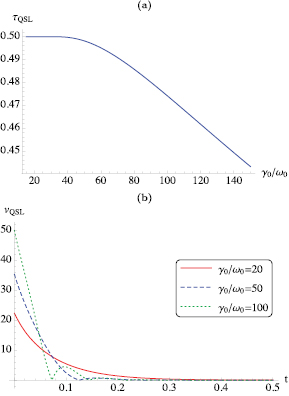
Figure 3. Quantum speed limit time ![$ \newcommand{\mrm}[1]{{\rm #1}} \tau_\mrm{QSL}$](https://content.cld.iop.org/journals/1751-8121/50/45/453001/revision2/aaa86c6ieqn207.gif) (82) (upper panel, (a)) and quantum speed limit
(82) (upper panel, (a)) and quantum speed limit ![$ \newcommand{\mrm}[1]{{\rm #1}} v_\mrm{QSL}$](https://content.cld.iop.org/journals/1751-8121/50/45/453001/revision2/aaa86c6ieqn208.gif) (81) (lower panel, (b)) for the damped-Jaynes–Cummings model (91) and the initial state
(81) (lower panel, (b)) for the damped-Jaynes–Cummings model (91) and the initial state  (96). Parameters are
  ,
,  and
and  .
.
Download figure:
Standard image High-resolution imageAs noted in [33] we observe that ![$ \newcommand{\mrm}[1]{{\rm #1}} \tau_\mrm{QSL}$](https://content.cld.iop.org/journals/1751-8121/50/45/453001/revision2/aaa86c6ieqn213.gif) is indeed monotonically decreasing as a function of the coupling strength,
is indeed monotonically decreasing as a function of the coupling strength,  . In the lower panel, we show the quantum speed limit
 ![$ \newcommand{\mrm}[1]{{\rm #1}} v_\mrm{QSL}$](https://content.cld.iop.org/journals/1751-8121/50/45/453001/revision2/aaa86c6ieqn215.gif) (81) for different values of
(81) for different values of  . Notice that for strong coupling
 ![$ \newcommand{\mrm}[1]{{\rm #1}} v_\mrm{QSL}$](https://content.cld.iop.org/journals/1751-8121/50/45/453001/revision2/aaa86c6ieqn217.gif) exhibits non-monotonic behaviour, which is a characteristic of non-Markovian dynamics.
exhibits non-monotonic behaviour, which is a characteristic of non-Markovian dynamics.
This observation was made more precise by Xu et al [146]. Without loss of generality they chose the qubit to be initially prepared in its excited state, ![$ \newcommand{\la}{\left\langle} \renewcommand{\bra}[1]{\left\langle #1\right\vert} \newcommand{\ra}{\right\rangle} \renewcommand{\ket}[1]{\left\vert #1\right\rangle} \rho_0=\ket{1}\bra{1}$](https://content.cld.iop.org/journals/1751-8121/50/45/453001/revision2/aaa86c6ieqn218.gif) . Denoting by Pt the population of the excited state one can then write,
. Denoting by Pt the population of the excited state one can then write,

This representation of the quantum speed limit time is particularly elucidating since it is closely related to a measure of non-Markovianity introduced by Breuer et al [147].
Generally, quantifying non-Markovianity is complicated [148, 149]. However, for simple quantum systems such as the Jaynes–Cummings model, equation (91), the situation drastically simplifies. Breuer et al [147] defined

where  are two initial states and

It has been seen [147] that for Markovian dynamics all initial states monotonically converge towards a unique stationary state. Thus, ![$ \newcommand{\si}[1]{\sin{\left(#1\right)}} \sigma(t, \rho_{1, 2}(0))$](https://content.cld.iop.org/journals/1751-8121/50/45/453001/revision2/aaa86c6ieqn220.gif) in equation (99) is strictly negative and
in equation (99) is strictly negative and ![$ \newcommand{\ma}[1]{\max{\left\{#1\right\}}} \newcommand{\mc}[1]{\mathcal{#1}} \mc{N}=0$](https://content.cld.iop.org/journals/1751-8121/50/45/453001/revision2/aaa86c6ieqn221.gif) , equation (98). Non-Markovian dynamics are characterised by an information backflow from the environment, and the convergence of
, equation (98). Non-Markovian dynamics are characterised by an information backflow from the environment, and the convergence of  towards the stationary state is accompanied by oscillations, cf non-monotonic behaviour of
 ![$ \newcommand{\mrm}[1]{{\rm #1}} v_\mrm{QSL}$](https://content.cld.iop.org/journals/1751-8121/50/45/453001/revision2/aaa86c6ieqn223.gif) in figure 3(b). Hence,
in figure 3(b). Hence, ![$ \newcommand{\si}[1]{\sin{\left(#1\right)}} \sigma(t, \rho_{1, 2}(0))$](https://content.cld.iop.org/journals/1751-8121/50/45/453001/revision2/aaa86c6ieqn224.gif) in equation (99) can become positive, which amounts to finite values of
in equation (99) can become positive, which amounts to finite values of ![$ \newcommand{\ma}[1]{\max{\left\{#1\right\}}} \newcommand{\mc}[1]{\mathcal{#1}} \mc{N}$](https://content.cld.iop.org/journals/1751-8121/50/45/453001/revision2/aaa86c6ieqn225.gif) .
.
It is then easy to see [146] that the quantum speed limit time, equation (97) reads,

Equation (100) clearly demonstrates that the more non-Markovian the dynamics, the faster a quantum system can evolve. Similar conclusions where found by Zhang et al for Ohmic spectral densities [150] and nonequilibrium environments [151]. However, it was also pointed out that the expression for ![$ \newcommand{\mrm}[1]{{\rm #1}} \tau_\mrm{QSL}$](https://content.cld.iop.org/journals/1751-8121/50/45/453001/revision2/aaa86c6ieqn226.gif) , and hence its behaviour sensitively depends on the choice of the initial state [152], which was confirmed by Zhu and Xu [153]. Moreover, quantum speed-ups can also be achieved by a judicious choice of the external driving protocol [154]. Finally, Liu et al [155] showed that in addition to non-Markovianity, the preparation of the initial state, and the choice of the driving protocol, the characteristics of the energy spectrum govern the maximal speed of quantum evolution. Finally, it is worth noting that the quantum speed limit time also sets the time-scale over which decoherence is effective [30, 156, 157].
, and hence its behaviour sensitively depends on the choice of the initial state [152], which was confirmed by Zhu and Xu [153]. Moreover, quantum speed-ups can also be achieved by a judicious choice of the external driving protocol [154]. Finally, Liu et al [155] showed that in addition to non-Markovianity, the preparation of the initial state, and the choice of the driving protocol, the characteristics of the energy spectrum govern the maximal speed of quantum evolution. Finally, it is worth noting that the quantum speed limit time also sets the time-scale over which decoherence is effective [30, 156, 157].
5.3.5. Environment assisted speed-up in cavity QED.
All this theoretical work posed the natural question whether environment assisted speed-ups could be observed in an experiment. Motivated by the theoretical study of the Jaynes–Cummings model [33], Cimmarusti et al [34] set out to test whether a similar effect could be observed in cavity QED. To accomplish this feat, however, Cimmarusti et al [34] had to deviate from the conventional view on cavity QED systems. More specifically, Cimmarusti et al [34] considered the cavity field as the 'system', and treated the atomic number that generates the atomic polarisation as a tuneable environment with a range of coupling constants. As a main result they found that varying the interaction strength of the optical cavity field with the environment by tuning the number of atoms modifies the time-dependent, nonclassical intensity correlation function. Moreover, the rate of evolution of the cavity field enhances—speeds up—with increasing the coupling. Finally, it was also shown [34] that the cavity field undergoes non-Markovian dynamics, and that the environment assisted speed-up is an effect of the non-Markovianity. Hence, Cimmarusti et al [34] experimentally verified the theoretical predictions.
This experiment has inspired several other studies including the work by Xu [158] on how to detect speed-ups in arbitrary systems and by Mo et al on engineering multiple environments [159].
5.4. Dynamics of multi-particle systems
Non-Markovianity can arise from collaborative excitations and correlations in the environment [160] (see Ref. [161] for a recent review of non-Markovian dynamics). Thus from studying the effect of correlations in its environment on the speed of a quantum system it is only natural to also analyse the influence of collaborative effects in the system itself. For instance, Liu et al [162] found that a open multi-qubit systems still exhibits the non-Markovian speed-up, but that also correlations intrinsic to the system can have the same effect. Similar effects were found in many level systems with avoided crossings by Poggi et al [163, 164], and by Hou et al for environments with star geometry [165] and finite XY spin chains [166]. Moreover, Song et al [167] found that these cooperative effects can be enhanced by a judicious choice of the external driving. Other speed-up mechanisms include criticality [168, 169] and initial correlations between system and environment [170].
5.4.1. The Lipkin–Meshkov–Glick bath.
When studying multi-particle quantum systems it becomes inevitable to also consider quantum phase transitions. Generically, quantum phase transitions are accompanied by a critical slowing down close to the critical point [171, 172]. Therefore, the behavior of the quantum speed limit ![$ \newcommand{\mrm}[1]{{\rm #1}} v_\mrm{QSL}$](https://content.cld.iop.org/journals/1751-8121/50/45/453001/revision2/aaa86c6ieqn227.gif) should be a good indicator of criticality. To make this observation more precise Hou et al [173] computed the quantum speed limit for a spin coupled to a LMG bath. The LMG model was originally introduced to describe the tunneling of bosons between degenerate levels in nuclei [174], but it recently attracted attention as a testbed for shortcuts to adiabaticity [175] and for quantum thermodynamics [176].
should be a good indicator of criticality. To make this observation more precise Hou et al [173] computed the quantum speed limit for a spin coupled to a LMG bath. The LMG model was originally introduced to describe the tunneling of bosons between degenerate levels in nuclei [174], but it recently attracted attention as a testbed for shortcuts to adiabaticity [175] and for quantum thermodynamics [176].
In Hou et al's [173] analysis the total Hamiltonian is given by

with

where ![$ \newcommand{\si}[1]{\sin{\left(#1\right)}} \sigma^\alpha$](https://content.cld.iop.org/journals/1751-8121/50/45/453001/revision2/aaa86c6ieqn228.gif) and
and ![$ \newcommand{\si}[1]{\sin{\left(#1\right)}} \sigma_i^\alpha$](https://content.cld.iop.org/journals/1751-8121/50/45/453001/revision2/aaa86c6ieqn229.gif) ,
,  are the Pauli matrices of the central spin and the ith spin of the bath. Note that HS can be understood as a probe system, which interacts through
  with the LMG-model HB. It is further easy to see [173] that HB undergoes a quantum phase transition for
  , where the symmetry is broken for
  . The question is now, if the quantum speed limit for the probe system only,
 ![$ \newcommand{\ptr}[2]{{\rm tr_{#1}}\left\{#2\right\}} \rho_S(t)=\ptr{B}{\rho_{tot}(t)}$](https://content.cld.iop.org/journals/1751-8121/50/45/453001/revision2/aaa86c6ieqn234.gif) , exhibits features of the phase transition in the environment. Hou et al [173] showed that this is indeed the case. Initialising the probe qubit in its excited state Hou et al examined the corresponding quantum speed limit time, as defined by Deffner and Lutz [33], fixing the evolution time
, exhibits features of the phase transition in the environment. Hou et al [173] showed that this is indeed the case. Initialising the probe qubit in its excited state Hou et al examined the corresponding quantum speed limit time, as defined by Deffner and Lutz [33], fixing the evolution time  . By weakly coupling to the LMG environment and determining the corresponding
  they showed that if the bath is in the symmetry broken phase, the probe evolves at (or close to for larger systems) the quantum speed limit. This reflects the large spectral gap present in this phase, see for example [176]. Conversely, when the bath is characterised by the symmetric phase, where the spectral gap becomes vanishingly small with system size,
  witnesses a significant drop. Therefore we can conclude that the dynamics of the probe is now significantly slower than
  . Interestingly we see
  in the vicinity of the critical point, thus reflecting the characteristic critical slowing down mentioned previously. These features are clearly shown in figure 4. Hou et al further explored the relationship between the behaviour of the quantum speed limit and the non-Markovian features induced by the bath [173].

Figure 4. Quantum speed limit time for a single qubit, initially in its excited state, weakly coupled to an LMG bath as given by equation (102). We fix  ,
,  , and
, and  . In the symmetry broken phase the probe evolves at the quantum speed limit, while in the symmetric phase the dynamics are significantly slower. Remarkably, near the critical point
  clearly spotlighting the quantum phase transition occurring in the bath.
Download figure:
Standard image High-resolution image5.5. Quantum speed limits for other quantities
Conventionally, geometric quantum speed limits are derived as upper bounds on the rate of change of a geometric measure of distinguishability. In the preceding sections we presented the case for the Bures angle, which is the generalised geometric angle between density operators. However, for many applications one is not necessarily interested in how exactly the quantum states evolve, but one rather needs a quick estimate of, for instance, the typical flow of entropy [177] or the rate of decoherence [178]. Thus, a plethora of other speed limits has been discussed in the literature.
A particularly insightful treatment was proposed by Uzdin and Kosloff [179]. Imagine that a system is initially prepared in a pure state, and then left to evolve under open system dynamics, for which the general master equation (65) becomes

with  for Markovian systems. Then its rate of decoherence, or more generally its rate of thermalisation, is characterised by the dynamics of the purity

Using the triangle inequality and the Cauchy–Schwarz inequality Uzdin and Kosloff [179] then find

The latter can be re-written to define a quantum speed limit time,

Equation (106) can be interpreted as a Mandelstam–Tamm type bound for the rate with which the purity, ![$ \newcommand{\ma}[1]{\max{\left\{#1\right\}}} \newcommand{\mc}[1]{\mathcal{#1}} \mc{P}(t)$](https://content.cld.iop.org/journals/1751-8121/50/45/453001/revision2/aaa86c6ieqn245.gif) , decays in open systems. Note that the denominator in equation (106) only depends on the Lindblad operators, and thus the resulting quantum speed limit time,
, decays in open systems. Note that the denominator in equation (106) only depends on the Lindblad operators, and thus the resulting quantum speed limit time, ![$ \newcommand{\ma}[1]{\max{\left\{#1\right\}}} \newcommand{\mc}[1]{\mathcal{#1}} \newcommand{\mrm}[1]{{\rm #1}} \tau_\mrm{QSL}^\mc{P}$](https://content.cld.iop.org/journals/1751-8121/50/45/453001/revision2/aaa86c6ieqn246.gif) , is independent of the time-dependent quantum states
, is independent of the time-dependent quantum states  .
.
A Margolus–Levitin type bound follows from re-writing the density operator in Liouville space, i.e.  is re-shaped as a vector in
 ![$ \newcommand{\ra}{\right\rangle} \renewcommand{\ket}[1]{\left\vert #1\right\rangle} \newcommand{\ma}[1]{\max{\left\{#1\right\}}} \newcommand{\mb}[1]{{\boldsymbol #1}} \newcommand{\mbb}[1]{\mathbb{#1}} \ket{\rho_t}\in\mbb{C}^{1\times N^2}$](https://content.cld.iop.org/journals/1751-8121/50/45/453001/revision2/aaa86c6ieqn249.gif) , and we have
, and we have ![$ \newcommand{\ra}{\right\rangle} \renewcommand{\ket}[1]{\left\vert #1\right\rangle} \newcommand{\ma}[1]{\max{\left\{#1\right\}}} \newcommand{\mc}[1]{\mathcal{#1}} \ket{\dot{\rho_t}}=\mc{H}\ket{\rho_t}$](https://content.cld.iop.org/journals/1751-8121/50/45/453001/revision2/aaa86c6ieqn250.gif) , where the Hamiltonian superoperator is given by [180]
, where the Hamiltonian superoperator is given by [180]

Here the  -product is defined as [180],

It then follows in complete analogy to above (see equations (80)–(83)) that we have,

and hence we obtain for the quantum speed limit time,

Accordingly a unified quantum speed limit time based on the dynamics of the purity becomes,

Similarly to the case of speed limits based on the Bures angle (89) Uzdin and Kosloff [179] again find that the Margolus–Levitin type bound (110) is tighter, but that the Mandelstam–Tamm type bound (106) is much easier to compute. This is illustrated by Uzdin and Kosloff [179] among other examples for dephasing channels and erasure of classical and quantum correlations.
The quantum speed limit based on the dynamics of the purity (111) serves as an important and illustrative example of various studies. Other examples include: Dehdashti et al [181] used the quantum speed limit based on the relative purity [32] to study decoherence in the spin-deformed boson model, whereas Jing et al [182] quantified the generation of quantumness. On the other hand, Mondal et al [183], as well as Pires et al [184], Marvian and Lidar [185], and Marvian et al [186] focused on the loss of quantum coherence in isolated and open dynamics. Finally, Sun et al [187] focused on computable bounds.
5.6. Universal, geometric quantum speed limits
Comparing the expressions for the quantum speed limit time, ![$ \newcommand{\mrm}[1]{{\rm #1}} \tau_\mrm{QSL}$](https://content.cld.iop.org/journals/1751-8121/50/45/453001/revision2/aaa86c6ieqn252.gif) , based on the Bures angle (89) and based on the purity equation (111), as well as the expressions for the relative purity [32] and the Winger–Yanase information [135] we notice that the choice of the measure of distinguishability only determines the numerator. The actual speed limit is set in all of these cases by a time-averaged Schatten-p-norm of the generator of the dynamics. This observation can be made more precise, if one starts the derivation of the speed limit directly with such a norm [188].
, based on the Bures angle (89) and based on the purity equation (111), as well as the expressions for the relative purity [32] and the Winger–Yanase information [135] we notice that the choice of the measure of distinguishability only determines the numerator. The actual speed limit is set in all of these cases by a time-averaged Schatten-p-norm of the generator of the dynamics. This observation can be made more precise, if one starts the derivation of the speed limit directly with such a norm [188].
To this end, consider the Schatten-p-distance

where p is an arbitrary, positive, real number. For  we have the Hilbert–Schmidt distance, for
  the trace distance, and for
  the operator norm.
The universal geometric speed (72) can be written as

The latter expression looks rather involved, but it can be simplified by using,  and employing the triangle inequality for operators,
 ![$ \newcommand{\trace}[1]{{\rm tr}\left\{#1\right\}} \newcommand{\tr}{{\rm tr}} \vert \trace{A}\vert \leqslant \trace{\vert A\vert }$](https://content.cld.iop.org/journals/1751-8121/50/45/453001/revision2/aaa86c6ieqn257.gif) , to read
, to read

Equation (114) can be further simplified with the help of Hölder's inequality [189]

which is true for all  . Now choosing
  and
and  , for which
  , we obtain

where we defined a universal quantum speed limit, ![$ \newcommand{\mrm}[1]{{\rm #1}} v_\mrm{QSL}^{\,p} $](https://content.cld.iop.org/journals/1751-8121/50/45/453001/revision2/aaa86c6ieqn262.gif) —independent of the physical situation and considered quantities.
—independent of the physical situation and considered quantities.
However, computing most of the Schatten-p-norms is rather involved, since the singular values of the generator of the dynamics have to be determined. An equivalent, and much more tractable quantum speed limit can be derived, if one considers the quantum state in its Wigner representation instead,

It was shown in [188] that if one considers the rate of Wasserstein-p-distance

one can derive

The two expressions (116) and (119) are fully equivalent up to normalization [188].
In conclusion, it was shown in [188] that, independent of the choice of measure, the quantum speed is universally characterised by the Schatten-p-norm of the generator of the dynamics. Moreover, this Schatten-p-norm can be computed from the mathematically tractable Wasserstein-p-norm of the corresponding Wigner function.
5.7. Applications: shortcuts to adiabaticity
We conclude this section on the geometric approach by highlighting an important application that was recognised only very recently. In the area of quantum control so-called shortcuts to adiabaticity have become a prominent and active topic [89]. A shortcut to adiabaticity is a fast process with the same final state that would result from infinitely slow driving. Within only a few years a huge variety of techniques has been developed [90–92, 171, 175, 190–212].
Among all of these techniques transitionless quantum driving is unique. In its original formulation [90–92] one considers a time-dependent Hamiltonian  and constructs an additional counterdiabatic field,
  , such that the joint Hamiltonian
  drives the dynamics precisely through the adiabatic manifold of
  . Moreover,
  vanishes by construction in the beginning,
  , and and the end,
  , of the finite time process. At first glance, it seems that such an energetically free shortcut to adiabaticity could be implemented for any arbitrarily fast process of arbitrarily short duration τ. That this is not the case and how the quantum speed limit enters the picture was formalised by Campbell and Deffner [93].
One can construct  such that the adiabatic solution of
  is an exact solution of the dynamics generated by
  , and we have [88, 90–92]

where we denote the instantaneous eigenstates of  by
by ![$ \newcommand{\ra}{\right\rangle} \renewcommand{\ket}[1]{\left\vert #1\right\rangle} \ket{n_t}$](https://content.cld.iop.org/journals/1751-8121/50/45/453001/revision2/aaa86c6ieqn274.gif) . In [88] a family of functionals has been proposed to quantify the cost associated with implementing
. In [88] a family of functionals has been proposed to quantify the cost associated with implementing  . The simplest member of the family is given by the trace norm,
 ![$ \newcommand{\mrm}[1]{{\rm #1}} \Vert \cdot\Vert _\mrm{tr}$](https://content.cld.iop.org/journals/1751-8121/50/45/453001/revision2/aaa86c6ieqn276.gif) [88, 97, 213, 214],
[88, 97, 213, 214],

It is easy to see that for a single 2-level spin,  is proportional to the average power input [88], i.e.
  reduces to an orthogonal, magnetic field. More generally, C can be interpreted as the additional action arising from the counterdiabatic driving. Hence, the relation to the quantum speed limit becomes apparent, since loosely speaking the quantum speed limit time sets a lower bound on the action
 ![$ \newcommand{\si}[1]{\sin{\left(#1\right)}} \newcommand{\mrm}[1]{{\rm #1}} E\, \tau_\mrm{QSL}\simeq \hbar/2$](https://content.cld.iop.org/journals/1751-8121/50/45/453001/revision2/aaa86c6ieqn279.gif) [67].
[67].
It is easy to see [93], that in the case of transitionless quantum driving the instantaneous cost, i.e. the trace norm of the counterdiabatic Hamiltonian,  , reduces to

where we used that ![$ \renewcommand{\bra}[1]{\left\langle #1\right\vert} \newcommand{\la}{\left\langle} \newcommand{\ra}{\right\rangle} \renewcommand{\braket}[2]{\left\langle #1\vert #2\right\rangle} \newcommand{\pd}{\partial} \braket{\pd_t n_t}{n_t}=0$](https://content.cld.iop.org/journals/1751-8121/50/45/453001/revision2/aaa86c6ieqn281.gif) , which is true for all Hamiltonians with entirely discrete eigenvalue spectrum. We further note that
, which is true for all Hamiltonians with entirely discrete eigenvalue spectrum. We further note that ![$ \newcommand{\ra}{\right\rangle} \renewcommand{\ket}[1]{\left\vert #1\right\rangle} \ket{\psi_t}=\ket{n_t}$](https://content.cld.iop.org/journals/1751-8121/50/45/453001/revision2/aaa86c6ieqn282.gif) and
and  with
with  as given in equation (120). To determine the speed we require

where we employed again ![$ \renewcommand{\bra}[1]{\left\langle #1\right\vert} \newcommand{\la}{\left\langle} \newcommand{\ra}{\right\rangle} \renewcommand{\braket}[2]{\left\langle #1\vert #2\right\rangle} \newcommand{\pd}{\partial} \braket{\pd_t n_t}{n_t}=0$](https://content.cld.iop.org/journals/1751-8121/50/45/453001/revision2/aaa86c6ieqn285.gif) and where
and where  are the instantaneous eigenvalues.
Collecting equations (121)–(123) the maximal speed becomes

and the corresponding quantum speed limit time becomes

Equations (124) and (125) express, in a transparent and immediate way, the trade-off of speed and cost of a shortcut to adiabaticity. The faster a quantum system evolves along its adiabatic manifold, the higher is the cost of implementing the shortcut.
Related results were found by Santos and Sarandy [97, 213] in the context of quantum computation and by Funo et al [215] from the work fluctuations during the finite-time process.
6. Quantum speed limits in non-Schrödinger quantum mechanics
In the above sections we have been aiming to provide an overview over the various notions of a quantum speed limit in standard quantum mechanics. So far, we have always assumed that the dynamics of an isolated systems is described by the von-Neumann equation (8), and that open systems can be described by a quantum master equation (65).
In this section we will broaden the scope of the analysis, and discuss generalisations and applications of the quantum speed limit for dynamics that are beyond the applicability of the Schrödinger equation.
6.1. Relativistic systems and Dirac dynamics
As a first example we are interested in relativistic quantum dynamics described by the Dirac equation,

Here, ![$ \newcommand{\mb}[1]{{\boldsymbol #1}} \Psi(\mb{x}, t)$](https://content.cld.iop.org/journals/1751-8121/50/45/453001/revision2/aaa86c6ieqn287.gif) is the wave function of an electron with rest mass m and elementary charge e at position
is the wave function of an electron with rest mass m and elementary charge e at position ![$ \newcommand{\mb}[1]{{\boldsymbol #1}} \mb{x}=(x_1, x_2, x_3)$](https://content.cld.iop.org/journals/1751-8121/50/45/453001/revision2/aaa86c6ieqn288.gif) , and c is the speed of light. Finally,
, and c is the speed of light. Finally,  is the vector-potential, with
 ![$ \newcommand{\mb}[1]{{\boldsymbol #1}} \mb{B}(\mb{x})=\nabla \times \mb{A}(\mb{x})$](https://content.cld.iop.org/journals/1751-8121/50/45/453001/revision2/aaa86c6ieqn290.gif) . In covariant form the matrices
. In covariant form the matrices ![$ \newcommand{\mb}[1]{{\boldsymbol #1}} \mb{\alpha}=(\alpha_1, \alpha_2, \alpha_3)$](https://content.cld.iop.org/journals/1751-8121/50/45/453001/revision2/aaa86c6ieqn291.gif) and
and  can be expressed as [216, 217],

The γ-matrices are commonly written in terms of  sub-matrices with the Pauli-matrices
 ![$ \newcommand{\si}[1]{\sin{\left(#1\right)}} \sigma_x, \sigma_y, \sigma_z$](https://content.cld.iop.org/journals/1751-8121/50/45/453001/revision2/aaa86c6ieqn294.gif) and the identity
and the identity ![$ \newcommand{\ma}[1]{\max{\left\{#1\right\}}} \newcommand{\id}{\mathbb{I}} \id_2$](https://content.cld.iop.org/journals/1751-8121/50/45/453001/revision2/aaa86c6ieqn295.gif) as,
as,

The solution of equation (126), the Dirac wave function ![$ \newcommand{\mb}[1]{{\boldsymbol #1}} \Psi(\mb{x}, t)$](https://content.cld.iop.org/journals/1751-8121/50/45/453001/revision2/aaa86c6ieqn296.gif) , is a bispinor, which can be interpreted as a superposition of a spin-up electron, a spin-down electron, a spin-up positron, and a spin-down positron [216, 217].
, is a bispinor, which can be interpreted as a superposition of a spin-up electron, a spin-down electron, a spin-up positron, and a spin-down positron [216, 217].
Since its inception [218] the Dirac equation (126) has proven to be one of the most versatile results of theoretical physics. Originally it was designed as a relativistic wave equation to describe massive spin- particles, such as electrons and quarks [216, 217]. Up to today, the Dirac equation enjoys plenty of attention [219–222], since it also found application in opto-mechanics [223], in quantum thermodynamics [224], and in condensed matter physics to describe so-called Dirac materials [225, 226].
It is only natural to ask whether and how the quantum speed limit generalises to relativistic Dirac dynamics. To this end, Villamizar and Duzzioni [227] further asked two specific questions: (i) which quantum states allow for the greatest spatial displacement in the shortest time, and (ii) can the relativistic quantum speed limit be used to (in-)validate a model for quantum dynamics.
To keep things as simple as possible Villamizar and Duzzioni [227] then considered systems in the x-y plane with ![$ \newcommand{\mb}[1]{{\boldsymbol #1}} \mb{B}(\mb{x})=B\, \hat{z}$](https://content.cld.iop.org/journals/1751-8121/50/45/453001/revision2/aaa86c6ieqn298.gif) , and an initial state that is is a homogeneous superposition of two radial eigenstates in different Landau energy levels. Thus, the initial states is of the form equation (18), for which the Mandelstam–Tamm and the Margolus–Levitin bound become identical and tight, and
, and an initial state that is is a homogeneous superposition of two radial eigenstates in different Landau energy levels. Thus, the initial states is of the form equation (18), for which the Mandelstam–Tamm and the Margolus–Levitin bound become identical and tight, and ![$ \newcommand{\mrm}[1]{{\rm #1}} \tau_\mrm{QSL}$](https://content.cld.iop.org/journals/1751-8121/50/45/453001/revision2/aaa86c6ieqn299.gif) (17) is the minimal time for the initial state to evolve to an orthogonal state.
(17) is the minimal time for the initial state to evolve to an orthogonal state.
If the dynamics was described by a Schrödinger equation we would have [227]

where E0 denotes the ground state energy. For the relativistic Dirac dynamics (126) we obtain [227]

where the second equality holds for strong magnetic fields,  , and where
  . Note that in the non-relativistic limit
 ![$ \newcommand{\mrm}[1]{{\rm #1}} \tau^S_\mrm{QSL}$](https://content.cld.iop.org/journals/1751-8121/50/45/453001/revision2/aaa86c6ieqn302.gif) and
and ![$ \newcommand{\mrm}[1]{{\rm #1}} \tau^D_\mrm{QSL}$](https://content.cld.iop.org/journals/1751-8121/50/45/453001/revision2/aaa86c6ieqn303.gif) become equivalent.
become equivalent.
It is then a simple exercise [227] to also compute the mean displacement, which can be written for Schrödinger dynamics as

and for Dirac dynamics in the ultra-relativistic limit

Combining the expressions for the quantum speed limit time equations (129)–(130) with the average displacements (131) and (131), we can define the average speed of an electron

We immediately see that for strong magnetic fields,  , the average speed computed from the Schrödinger dynamics can surpass the speed of light, c. As expected, this is not the case for the Dirac equation, and even for arbitrarily strong fields B we always have
  . Thus, Villamizar and Duzzioni [227] conclude that the quantum speed limit can be used to check the physical consistency of a physical model. Villamizar and Duzzioni's [227] work has been followed by several further analyses for which we refer the reader to the literature [228–231].
Finally, it is interesting to note that in passing Villamizar and Duzzioni [227] resolved the longstanding debate of Einstein and Bohr (see section 1) by bringing the energy-time uncertainty principle in full agreement with special relativity.
6.2. PT-symmetric quantum mechanics
Another area of research that has attracted considerable attention are non-Hermitian [232–236] and ![$ \newcommand{\ma}[1]{\max{\left\{#1\right\}}} \newcommand{\mc}[1]{\mathcal{#1}} \mc{PT}$](https://content.cld.iop.org/journals/1751-8121/50/45/453001/revision2/aaa86c6ieqn306.gif) -symmetric quantum systems [178, 237–240]. Since its originial development as a rather mathematical theory [237, 241],
-symmetric quantum systems [178, 237–240]. Since its originial development as a rather mathematical theory [237, 241], ![$ \newcommand{\ma}[1]{\max{\left\{#1\right\}}} \newcommand{\mc}[1]{\mathcal{#1}} \mc{PT}$](https://content.cld.iop.org/journals/1751-8121/50/45/453001/revision2/aaa86c6ieqn307.gif) -symmetric quantum mechanics has found experimental realisation as systems with balanced loss and gain [241–247].
-symmetric quantum mechanics has found experimental realisation as systems with balanced loss and gain [241–247].
In ![$ \newcommand{\ma}[1]{\max{\left\{#1\right\}}} \newcommand{\mc}[1]{\mathcal{#1}} \mc{PT}$](https://content.cld.iop.org/journals/1751-8121/50/45/453001/revision2/aaa86c6ieqn308.gif) -symmetric quantum mechanics the Hamiltonian H is non-Hermitian, but commutes with
-symmetric quantum mechanics the Hamiltonian H is non-Hermitian, but commutes with ![$ \newcommand{\ma}[1]{\max{\left\{#1\right\}}} \newcommand{\mc}[1]{\mathcal{#1}} \mc{P}$](https://content.cld.iop.org/journals/1751-8121/50/45/453001/revision2/aaa86c6ieqn309.gif) and
and ![$ \newcommand{\ma}[1]{\max{\left\{#1\right\}}} \newcommand{\mc}[1]{\mathcal{#1}} \mc{T}$](https://content.cld.iop.org/journals/1751-8121/50/45/453001/revision2/aaa86c6ieqn310.gif) , i.e.
, i.e. ![$ \newcommand{\ma}[1]{\max{\left\{#1\right\}}} \newcommand{\mc}[1]{\mathcal{#1}} \left[ \mc{PT}, H\right]=0$](https://content.cld.iop.org/journals/1751-8121/50/45/453001/revision2/aaa86c6ieqn311.gif) . Here,
. Here, ![$ \newcommand{\ma}[1]{\max{\left\{#1\right\}}} \newcommand{\mc}[1]{\mathcal{#1}} \mc{P}$](https://content.cld.iop.org/journals/1751-8121/50/45/453001/revision2/aaa86c6ieqn312.gif) is the space reflection (parity) operator, and
is the space reflection (parity) operator, and ![$ \newcommand{\ma}[1]{\max{\left\{#1\right\}}} \newcommand{\mc}[1]{\mathcal{#1}} \mc{T}$](https://content.cld.iop.org/journals/1751-8121/50/45/453001/revision2/aaa86c6ieqn313.gif) is the time-reflection operator [238],
is the time-reflection operator [238],

where x and p are position and momentum operators, respectively. Since ![$ \newcommand{\ma}[1]{\max{\left\{#1\right\}}} \newcommand{\mc}[1]{\mathcal{#1}} \mc{T}$](https://content.cld.iop.org/journals/1751-8121/50/45/453001/revision2/aaa86c6ieqn314.gif) also changes the sign of the imaginary unit i, canonical commutation relations such as
also changes the sign of the imaginary unit i, canonical commutation relations such as ![$ \newcommand{\com}[2]{\left[#1,\,#2\right]} \newcommand{\co}[1]{\cos{\left(#1\right)}} \com{x}{p}={\rm i}\hbar$](https://content.cld.iop.org/journals/1751-8121/50/45/453001/revision2/aaa86c6ieqn315.gif) are invariant under
are invariant under ![$ \newcommand{\ma}[1]{\max{\left\{#1\right\}}} \newcommand{\mc}[1]{\mathcal{#1}} \mc{PT}$](https://content.cld.iop.org/journals/1751-8121/50/45/453001/revision2/aaa86c6ieqn316.gif) .
.
The major difference between Hermitian and ![$ \newcommand{\ma}[1]{\max{\left\{#1\right\}}} \newcommand{\mc}[1]{\mathcal{#1}} \mc{PT}$](https://content.cld.iop.org/journals/1751-8121/50/45/453001/revision2/aaa86c6ieqn317.gif) -symmetric quantum mechanics is the definition of the inner product [238, 248]. For Hermitian Hamiltonians we have,
-symmetric quantum mechanics is the definition of the inner product [238, 248]. For Hermitian Hamiltonians we have,

where, as usual, † denotes conjugate transpose. This inner product, however, results in indefinite norms for the non-Hermitian, but ![$ \newcommand{\ma}[1]{\max{\left\{#1\right\}}} \newcommand{\mc}[1]{\mathcal{#1}} \mc{PT}$](https://content.cld.iop.org/journals/1751-8121/50/45/453001/revision2/aaa86c6ieqn318.gif) -symmetric case [238]. This observation will become crucial below, since this means that for the geometric approach the angle (67) will have to be re-defined.
-symmetric case [238]. This observation will become crucial below, since this means that for the geometric approach the angle (67) will have to be re-defined.
In ![$ \newcommand{\ma}[1]{\max{\left\{#1\right\}}} \newcommand{\mc}[1]{\mathcal{#1}} \mc{PT}$](https://content.cld.iop.org/journals/1751-8121/50/45/453001/revision2/aaa86c6ieqn319.gif) -symmetric quantum mechanics the inner product is defined in terms of the metric operator
-symmetric quantum mechanics the inner product is defined in terms of the metric operator ![$ \newcommand{\ma}[1]{\max{\left\{#1\right\}}} \newcommand{\mc}[1]{\mathcal{#1}} \mc{C}$](https://content.cld.iop.org/journals/1751-8121/50/45/453001/revision2/aaa86c6ieqn320.gif) as [238]
as [238]

In the unbroken regime, i.e. if the eigenvalues of H are real, ![$ \newcommand{\ma}[1]{\max{\left\{#1\right\}}} \newcommand{\mc}[1]{\mathcal{#1}} \mc{C}$](https://content.cld.iop.org/journals/1751-8121/50/45/453001/revision2/aaa86c6ieqn321.gif) can be determined from [238],
can be determined from [238],

Note that the time evolution induced by a time-independent Hamiltonian with real eigenvalues is unitary. Thus, one would naively expect that both the Mandelstam–Tamm (12) as well as the Margolus–Levitin bound (16) for time-dependent generators to remain valid.
To analyse this claim Bender et al [249] considered a simple case study. Imagine a qubit, which is initially prepared in ![$ \newcommand{\ra}{\right\rangle} \renewcommand{\ket}[1]{\left\vert #1\right\rangle} \ket{\psi_0}$](https://content.cld.iop.org/journals/1751-8121/50/45/453001/revision2/aaa86c6ieqn322.gif) and we want to drive it to the final state
and we want to drive it to the final state ![$ \newcommand{\ra}{\right\rangle} \renewcommand{\ket}[1]{\left\vert #1\right\rangle} \ket{\psi_T}$](https://content.cld.iop.org/journals/1751-8121/50/45/453001/revision2/aaa86c6ieqn323.gif) with
with

The most general, but ![$ \newcommand{\ma}[1]{\max{\left\{#1\right\}}} \newcommand{\mc}[1]{\mathcal{#1}} \mc{PT}$](https://content.cld.iop.org/journals/1751-8121/50/45/453001/revision2/aaa86c6ieqn324.gif) -symmetric Hamiltonian can be written as
-symmetric Hamiltonian can be written as

and thus the final state, ![$ \newcommand{\ra}{\right\rangle} \renewcommand{\ket}[1]{\left\vert #1\right\rangle} \ket{\psi_T}$](https://content.cld.iop.org/journals/1751-8121/50/45/453001/revision2/aaa86c6ieqn325.gif) , reads [249]
, reads [249]

where α and ω are determined by ![$ \newcommand{\si}[1]{\sin{\left(#1\right)}} \si{\alpha}=r \si{\theta}/s$](https://content.cld.iop.org/journals/1751-8121/50/45/453001/revision2/aaa86c6ieqn326.gif) and
and ![$ \newcommand{\si}[1]{\sin{\left(#1\right)}} \omega^2=4s^2-4 r^2\sin^2{(\theta)}$](https://content.cld.iop.org/journals/1751-8121/50/45/453001/revision2/aaa86c6ieqn327.gif) , respectively.
, respectively.
Bender et al [249] then argued that ![$ \newcommand{\ma}[1]{\max{\left\{#1\right\}}} \newcommand{\mc}[1]{\mathcal{#1}} \mc{PT}$](https://content.cld.iop.org/journals/1751-8121/50/45/453001/revision2/aaa86c6ieqn328.gif) -symmetric Hamiltonians provide means to accelerate quantum mechanics. For instance, if we chose
-symmetric Hamiltonians provide means to accelerate quantum mechanics. For instance, if we chose  and
and  in equation (138) then equation (140) suggests that the quantum system could evolve from
 ![$ \newcommand{\ra}{\right\rangle} \renewcommand{\ket}[1]{\left\vert #1\right\rangle} \ket{\psi_0}$](https://content.cld.iop.org/journals/1751-8121/50/45/453001/revision2/aaa86c6ieqn331.gif) to
to ![$ \newcommand{\ra}{\right\rangle} \renewcommand{\ket}[1]{\left\vert #1\right\rangle} \ket{\psi_T} $](https://content.cld.iop.org/journals/1751-8121/50/45/453001/revision2/aaa86c6ieqn332.gif) in arbitrarily short times. However, Bender et al [249] also note that such
in arbitrarily short times. However, Bender et al [249] also note that such ![$ \newcommand{\ra}{\right\rangle} \renewcommand{\ket}[1]{\left\vert #1\right\rangle} \ket{\psi_0}$](https://content.cld.iop.org/journals/1751-8121/50/45/453001/revision2/aaa86c6ieqn333.gif) and
and ![$ \newcommand{\ra}{\right\rangle} \renewcommand{\ket}[1]{\left\vert #1\right\rangle} \ket{\psi_T} $](https://content.cld.iop.org/journals/1751-8121/50/45/453001/revision2/aaa86c6ieqn334.gif) are no longer orthogonal, since under
are no longer orthogonal, since under ![$ \newcommand{\ma}[1]{\max{\left\{#1\right\}}} \newcommand{\mc}[1]{\mathcal{#1}} \mc{PT}$](https://content.cld.iop.org/journals/1751-8121/50/45/453001/revision2/aaa86c6ieqn335.gif) -symmetric Hamiltonians the inner product, and hence the geometry of Hilbert space has to be modified (137).
-symmetric Hamiltonians the inner product, and hence the geometry of Hilbert space has to be modified (137).
Thus, Uzdin et al [250] revisited the geometric approach to the quantum speed limit. As a starting point of their analysis they consider the angle ![$ \newcommand{\ma}[1]{\max{\left\{#1\right\}}} \newcommand{\mc}[1]{\mathcal{#1}} \mc{L}$](https://content.cld.iop.org/journals/1751-8121/50/45/453001/revision2/aaa86c6ieqn336.gif) between two arbitrary, complex vectors
between two arbitrary, complex vectors ![$ \newcommand{\ra}{\right\rangle} \renewcommand{\ket}[1]{\left\vert #1\right\rangle} \ket{\psi_1}$](https://content.cld.iop.org/journals/1751-8121/50/45/453001/revision2/aaa86c6ieqn337.gif) and
and ![$ \newcommand{\ra}{\right\rangle} \renewcommand{\ket}[1]{\left\vert #1\right\rangle} \ket{\psi_2}$](https://content.cld.iop.org/journals/1751-8121/50/45/453001/revision2/aaa86c6ieqn338.gif)

Note that generally ![$ \newcommand{\ra}{\right\rangle} \renewcommand{\ket}[1]{\left\vert #1\right\rangle} \ket{\psi_1}$](https://content.cld.iop.org/journals/1751-8121/50/45/453001/revision2/aaa86c6ieqn339.gif) and
and ![$ \newcommand{\ra}{\right\rangle} \renewcommand{\ket}[1]{\left\vert #1\right\rangle} \ket{\psi_2}$](https://content.cld.iop.org/journals/1751-8121/50/45/453001/revision2/aaa86c6ieqn340.gif) are not normalised. In complete analogy to above (see equations (26)–(30)) it can then be shown that
are not normalised. In complete analogy to above (see equations (26)–(30)) it can then be shown that

where ![$ \renewcommand{\bra}[1]{\left\langle #1\right\vert} \renewcommand{\ket}[1]{\left\vert #1\right\rangle} \newcommand{\la}{\left\langle} \newcommand{\ra}{\right\rangle} \renewcommand{\braket}[2]{\left\langle #1\vert #2\right\rangle} \newcommand{\e}{{\rm e}} \ket{\Psi}\equiv \ket{\psi(t)}/\sqrt{\braket{\psi(t)}{\psi(t)}}$](https://content.cld.iop.org/journals/1751-8121/50/45/453001/revision2/aaa86c6ieqn341.gif) . Repeating the by now familiar steps Uzdin et al [250] find that a quantum speed limit for non-Hermitian systems can be written in complete analogy to Hermitian systems as
. Repeating the by now familiar steps Uzdin et al [250] find that a quantum speed limit for non-Hermitian systems can be written in complete analogy to Hermitian systems as

where we here have

and N is the dimension of the Hilbert space of H. In their analysis Uzdin et al [250] then use equation (143) to identify time-optimal Hamiltonians, for which the fastest evolution between specific initial and final states can be achieved.
Identifying time-optimal Hamiltonians is sometimes also dubbed the quantum brachistochrone problem, which has been further elaborated in the literature for Hermitian [251–257] as well as non-Hermitian systems [258–264].
6.3. Non-linear systems
Finally, the notion of quantum speed limits has also been generalised to non-linear systems. Non-linear Schrödinger equations arise from effective descriptions of many-particle systems, such as Bose–Einstein condensates (BEC) [265] or in non-linear optics [266]. Consequently, Chen et al [267] generalised Hergerfeldt's earlier work [116, 132] to two models, namely one describing standard BECs,

where where  and
and  are probability amplitudes of two possible states, κ describes the interaction between atoms, and
  and
and  energy bias and coupling strength. The second model is more involved and describes oscillations between atomic and molecular BECs.
It had been claimed by Dou et al [268] that nonlinear interactions strongly affect the minimal time a quantum system needs to evolve between distinct states. This claim was refuted by Chen et al [267], and they showed explicitly that the maximal quantum speed of nonlinear systems for unconstrained controls is independent of the strength of the non-linearity, and that non-linear systems at maximal speed evolve as fast as equivalent linear systems. In particular, they found for unconstrained control protocols  ,
,

where  and
and  are initial and final azimuth on the Bloch sphere. Note that
 ![$ \newcommand{\mrm}[1]{{\rm #1}} \tau_\mrm{min}$](https://content.cld.iop.org/journals/1751-8121/50/45/453001/revision2/aaa86c6ieqn349.gif) is independent of κ and that
is independent of κ and that ![$ \newcommand{\mrm}[1]{{\rm #1}} \tau_\mrm{min}$](https://content.cld.iop.org/journals/1751-8121/50/45/453001/revision2/aaa86c6ieqn350.gif) is similar to the result for linear qubits with more than one control parameter (64).
is similar to the result for linear qubits with more than one control parameter (64).
7. Relation to other fundamental bounds
7.1. Cramer–Rao bound and beyond
From section 3.4 we have already established that a strict relationship exists between certain formulations of the quantum speed limit and the quantum Fisher information, and therefore with the quantum Cramer–Rao bound. As alluded to earlier, the existence of a tight relationship is natural: Heisenberg's uncertainty principles limits the accuracy with which we can measure conjugate variables, while the Cramer–Rao bound tells us that no procedure for estimating the value of a given quantity can have a precision scaling better than the inverse of the standard deviation of a conjugate quantity. Therefore, while the quantum speed limit arises by virtue of the energy-time uncertainty relation, in principle we can use the same reasoning for any pair of conjugate variables. This approach was recently followed in order to re-examine the measurement precision bounds by Giovannetti, Lloyd, and Maccone [269]. Interestingly, while the Cramer–Rao bound is asymptotically tight (in the number of measurements performed), for moderate numbers of measurements this line of reasoning leads to a tighter bound.
If the parameter to estimate, μ, is encoded in some state, the quantum fluctuations associated with this can be connected to a conjugate operator, H, that generates translations of μ,  . We remark, H can be, although is not necessarily, the Hamiltonian of the system at hand. Assuming there are M copies of the state, along with pure probe states and a unitary encoding scheme, we can establish the quantum Cramer–Rao bound takes the form

In [269] the authors derive an alternative bound on the root mean squared error for μ

where E0 is the minimum eigenvalue of H and κ is a constant. To establish equation (148) the authors use the fact that a 'quantum speed limit' in this instance, which links the fidelity, F, of the states for values of the parameter μ and  to the difference
  through the mapping
  , is given by

where  from [71]. These functions can then be bounded and optimised to show equation (148) [269].
Of course, in the situation where the parameter to estimate is time and H corresponds to the system Hamiltonian, then the analysis reduces to the 'standard' quantum speed limit. However, the remarkable insight of [269] is that for any pair of conjugate variables this reasoning can be used to establish tight bounds on the precision with which they can be estimated.
7.2. Landauer's bound
It is widely accepted that information is not an abstract entity, but rather a physical quantity. In particular, Landauer established that in order to erase a single bit of information there is an associated minimum energetic cost, given by the dissipated heat [270, 271]

While the ramifications of this have lead to many significant insights regarding computational costs, the physical nature of information and a host of others, our interest lies in assessing its recent experimental verification. The first experiment was performed by Bérut et al [272], where they used a single colloidal particle trapped in a time-dependent double well potential. By modulating and tilting the potential slowly enough they were able to achieve Landauer limited bit erasure. Since then several other experiments have tested and verified equation (150) in a variety of settings both classical and quantum [273–276]. However, most of these experiments shared one common aspect, namely that the erasure processes was performed slowly in order to avoid generating excess excitations and therefore costing more energy. Considering the discussions of section 3.3, since Landauer's bound sets a minimal energy to transition between two orthogonal states, it therefore seems to naturally lend itself to exploring the quantum speed limit, provided the information is encoded into a quantum system. In fact, as shown in [272] where the erasure protocol was classical, they approach the Landauer limit only asymptotically with increasing cycle duration.
The recent experiment by Gaudenzi et al [276], however, explicitly considered a quantum set-up. In this case, Landauer's bound sets the minimal energy and the quantum speed limit, essentially independently, sets the minimal time to achieve the erasure. Using the energy-time uncertainty relation they established that the quantum limit is given by

By exploiting quantum tunnelling to realise a carefully controlled evolution, they were able to achieve Landauer limited bit erasure several orders of magnitude faster (although not yet at the quantum speed limit) than any previous implementations.
7.3. Lieb–Robinson bound
We saw in section 4.1.1 that the quantum speed limit fundamentally bounds the rate at which a quantum state can be communicated along a quantum channel. Indeed, while the emergence of  is remarkable, the fact that information cannot propagate arbitrarily fast when the interaction range is limited is quite intuitive. In fact, this notion is formalised in the form of Lieb–Robinson bounds [114]. In essence, these bounds set constraints on the speed with which local effects can propagate through a quantum system by rigorously showing that correlations between the expectation values of local observables are exponentially suppressed outside an effective 'space-time cone'. We refer to [277] for an introduction to the more formal aspects of Lieb–Robinson bounds and some of their more far reaching implications.
If we consider only nearest-neighbour interactions, then the speed with which correlations can travel along a one-dimensional chain is bounded linearly by the so-called Lieb–Robinson velocity, vLR. This behaviour was recently verified experimentally in [278], while the analysis for long range interactions, where such bounds can be violated is found in [118]. To the best of our knowledge, it is currently an open question regarding a more stringent relation between vLR and the speed arising from the quantum speed limit, vQSL.
7.4. Maximal rate of quantum learning and Holevo's information
As a final example we return to the Bremerman–Bekenstein bound (36). In its original formulation it gives an upper bound on the rate with which information can be extracted from a quantum system. However, the bound is rather weak, since it assumes that the total information stored in the quantum system is accessible. Generally this is not the case [279] due to the quantum back action of measurements [280].
Imagine that we have an observable  , where an are the measurement outcomes, and
  are the projectors into the eigenspaces corresponding to an. Generally, the post-measurement quantum state ρ will suffer from a back-action, i.e, information about the quantum system will be lost in the measurement. How much information is lost is quantified by Holevo's information,

where ![$ \newcommand{\trace}[1]{{\rm tr}\left\{#1\right\}} \newcommand{\loge}[1]{\ln{\left(#1\right)}} \newcommand{\tr}{{\rm tr}} S(\rho)=-\trace{\rho \loge{\rho}}$](https://content.cld.iop.org/journals/1751-8121/50/45/453001/revision2/aaa86c6ieqn359.gif) is the von-Neumann entropy, and
is the von-Neumann entropy, and  is the post-measurement state. Further,
 ![$ \newcommand{\trace}[1]{{\rm tr}\left\{#1\right\}} \newcommand{\ma}[1]{\max{\left\{#1\right\}}} \newcommand{\mf}[1]{\mathfrak{#1}} \newcommand{\tr}{{\rm tr}} \mf{p}_n=\trace{\Pi_n \rho}$](https://content.cld.iop.org/journals/1751-8121/50/45/453001/revision2/aaa86c6ieqn361.gif) denotes the probability to obtain the nth measurement outcome.
denotes the probability to obtain the nth measurement outcome.
Very recently, Acconcia and Deffner [281] then used χ to define the maximal rate of quantum learning. If χ is the accessible information, then a 'rate of learning' quantifies the change of χ under a time-dependent perturbation. In complete analogy to the Bremerman–Bekenstein bound one can then find an upper bound on the rate with which the accessible information changes by

In [281] this bound was studied for the harmonic oscillator and for the Pöschl–Teller potential by means of time-dependent perturbation theory.
8. Final remarks
Throughout this topical review we have striven to focus on the practical applications of the quantum speed limit. In particular, with the rapid development of new quantum technologies and the recent surge of interest in exploring the thermodynamic working principles of quantum systems it is important to understand the limits on controlling such systems. Arguably the most basic question one can ask is: how fast can we achieve a desired outcome? To which one then naturally would attempt to reduce the time or, seemingly equivalently, speed up the process. Interestingly, these two approaches actually allow us to formulate and study the quantum speed limit in very different settings. In the former approach, while the establishment of the quantum speed limit time arises from the energy-time uncertainty principle, it is quite remarkable that precisely this time emerges as the minimal evolution time for optimised quantum systems. Employing the latter approach, based on the geometry of a quantum evolution, we were able to identify new and unexpected control mechanisms. In most set-ups for quantum computation one works hard to isolate the system against noise and decoherence from the environment. The geometric approach to quantum speed limits, however, indicated environmental correlations as a valuable resource to speed-up quantum processes. The implications are far reaching, in particular considering the development of quantum computers and quantum enhanced thermal devices, for which the quantum speed limit is crucial in characterising the associated limitations.
While of fundamental interest, arguably it is the practical ramifications of the energy-time uncertainty principle that has lead to the renewed interest. The diverse range of techniques to control quantum systems has allowed us to exploit the quantum speed limit to understand the limits of metrology, features of criticality, define the efficiency of quantum devices, and understand the cost of controlled quantum evolutions. Undoubtedly there are many more revelations to come, for instance in further developing the notion in non-standard quantum mechanics or a clearer understanding for complex multipartite systems. As we have tried to evidence in this topical review, the seeming ubiquity of the quantum speed limit in controlling quantum systems indicates more is to be learned.
We close with a more philosophical remark: quantum speed limits are an inherently quantum phenomenon with no classical analogue. The ramifications of such counter-intuitive, yet fundamental bounds of physical reality have puzzled the greatest among us—as highlighted by the long debates by Einstein and Bohr in the XX century. Over the last century, however, quantum theory has undoubtedly become the cornerstone of physics and its 'peculiarities' are what make the Universe work. To say it in Zurek's words [282]:
The only 'failure' of quantum theory is its inability to provide a natural framework for our prejudices about the workings of the Universe.
Acknowledgments
We are grateful to Marta Paczyńska for creating the visual representation of Einstein's gedankenexperiment, figure 1, and Lu (Lucy) Hou for providing the resources for figure 4. SD would like to thank Eric Lutz for many years of insightful discussions and supporting mentorship, and in particular for inciting our interest in quantum speed limits. This work was supported by the U.S. National Science Foundation under Grant No. CHE-1648973.
Footnotes
- 3
English translation of the German original: Die Quantenmechanik ist sehr achtung-gebietend. Aber eine innere Stimme sagt mir, daß das doch nicht der wahre Jakob ist. Die Theorie liefert viel, aber dem Geheimnis des Alten bringt sie uns kaum näher. Jedenfalls bin ich berzeugt, daß der nicht würfelt.
- 4
Without any mathematical justification Heisenberg explicitly writes [2],
. - 5

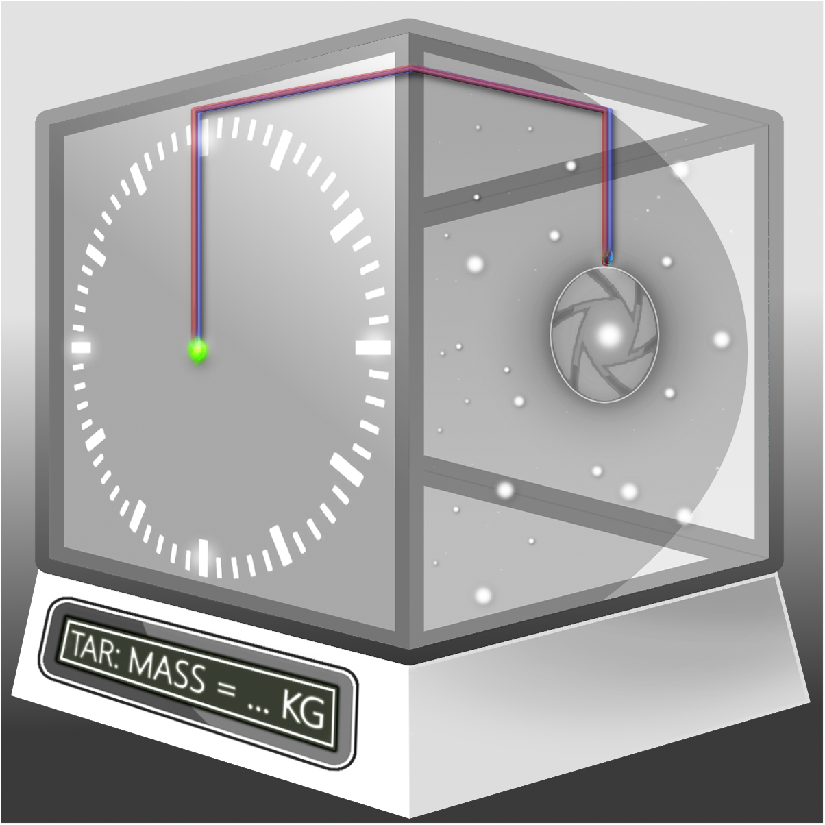