
Abstract
Quantum Fisher information matrix (QFIM) is a core concept in theoretical quantum metrology due to the significant importance of quantum Cramér–Rao bound in quantum parameter estimation. However, studies in recent years have revealed wide connections between QFIM and other aspects of quantum mechanics, including quantum thermodynamics, quantum phase transition, entanglement witness, quantum speed limit and non-Markovianity. These connections indicate that QFIM is more than a concept in quantum metrology, but rather a fundamental quantity in quantum mechanics. In this paper, we summarize the properties and existing calculation techniques of QFIM for various cases, and review the development of QFIM in some aspects of quantum mechanics apart from quantum metrology. On the other hand, as the main application of QFIM, the second part of this paper reviews the quantum multiparameter Cramér–Rao bound, its attainability condition and the associated optimal measurements. Moreover, recent developments in a few typical scenarios of quantum multiparameter estimation and the quantum advantages are also thoroughly discussed in this part.
Export citation and abstract BibTeX RIS

Original content from this work may be used under the terms of the Creative Commons Attribution 3.0 licence. Any further distribution of this work must maintain attribution to the author(s) and the title of the work, journal citation and DOI.
1. Introduction
After decades of rapid development, quantum mechanics has now gone deep into almost every corner of modern science, not only as a fundamental theory, but also as a technology. The technology originated from quantum mechanics is usually referred to as quantum technology, which is aiming at developing brand new technologies or improving current existing technologies with the association of quantum resources, quantum phenomena or quantum effects. Some aspects of quantum technology, such as quantum communications, quantum computation, quantum cryptography and quantum metrology, have shown great power in both theory and laboratory to lead the next industrial revolution. Among these aspects, quantum metrology is the most promising one that can step into practice in the near future.
Quantum metrology focuses on making high precision measurements of given parameters using quantum systems and quantum resources. Generally, a complete quantum metrological process contains four steps: (1) preparation of the probe state; (2) parameterzation; (3) measurement and (4) classical estimation, as shown in figure 1. The last step has been well studies in classical statistics, hence, the major concern of quantum metrology is the first three steps.
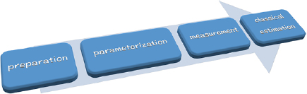
Figure 1. Schematic of a complete quantum metrological process, which contains four steps: (1) preparation of the probe state; (2) parameterzation; (3) measurement; (4) classical estimation.
Download figure:
Standard image High-resolution imageQuantum parameter estimation is the theory for quantum metrology, and quantum Cramér–Rao bound is the most well-studied mathematical tool for quantum parameter estimation [1, 2]. In quantum Cramér–Rao bound, the quantum Fisher information (QFI) and quantum Fisher information matrix (QFIM) are the key quantities representing the precision limit for single parameter and multiparameter estimations. In recent years, several outstanding reviews on quantum metrology and quantum parameter estimation have been provided from different perspectives and at different time, including the ones given by Giovannetti et al on the quantum-enhanced measurement [3] and the advances in quantum metrology [4], the ones given by Paris [5] and Toth et al [6] on the QFI and its applications in quantum metrology, the one by Braun et al on the quantum enhanced metrology without entanglement [7], the ones by Pezzè et al [8] and Huang et al [9] on quantum metrology with cold atoms, the one by Degen et al on general quantum sensing [10], the one by Pirandola et al on the photonic quantum sensing [11], the ones by Dowling on quantum optical metrology with high-N00N state [12] and Dowling and Seshadreesan on theoretical and experimental optical technologies in quantum metrology, sensing and imaging [13], the one by Demkowicz-Dobrzański et al on the quantum limits in optical interferometry [14], the one by Sidhu and Kok on quantum parameter estimation from a geometric perspective [15], and the one by Szczykulska et al on simultaneous multiparameter estimation [16]. Petz et al also wrote a thorough technical introduction on QFI [17].
Apart from quantum metrology, the QFI also connects to other aspects of quantum physics, such as quantum phase transition [18–20] and entanglement witness [21, 22]. The widespread application of QFI may be due to its connection to the Fubini-study metric, a Kähler metric in the complex projective Hilbert space. This relation gives the QFI a strong geometric meaning and makes it a fundamental quantity in quantum physics. Similarly, the QFIM shares this connection since the diagonal entries of QFIM simply gives the QFI. Moreover, the QFIM also connects to other fundamental quantity like the quantum geometric tensor [23]. Thus, besides the role in multiparameter estimation, the QFIM should also be treated as a fundamental quantity in quantum mechanics.
In recent years, the calculation techniques of QFIM have seen a rapid development in various scenarios and models. However, there lack papers that thoroughly summarize these techniques in a structured manner for the community. Therefore, this paper not only reviews the recent developments of quantum multiparameter estimation, but also provides comprehensive techniques on the calculation of QFIM in a variety of scenarios. For this purpose, this paper is presented in a way similar to a textbook with many technical details given in the appendices, which could help the readers to follow and better understand the corresponding results.
2. Quantum Fisher information matrix
2.1. Definition
Consider a vector of parameters  with xa the ath parameter.
  is encoded in the density matrix
  . In the entire paper we denote the QFIM as
  , and an entry of
  is defined as [1, 2]

where  represents the anti-commutation and La (Lb) is the symmetric logarithmic derivative (SLD) for the parameter xa (xb), which is determined by the equation6

The SLD operator is a Hermitian operator and the expected value  . Utilizing the equation above,
  can also be expressed by [24]

Based on equation (1), the diagonal entry of QFIM is

which is exactly the QFI for parameter xa.
The definition of Fisher information matrix originated from classical statistics. For a probability distribution  where
where  is the conditional probability for the outcome result y , an entry of Fisher information matrix is defined as

For discrete outcome results, it becomes ![$\mathcal{I}_{ab}:=\sum\nolimits_{y} \frac{[\partial_{a}p(y|\vec {x})][\partial_{b}p(y|\vec {x})]} {p(y|\vec {x})}$](https://content.cld.iop.org/journals/1751-8121/53/2/023001/revision2/aab5d4dieqn015.gif) . With the development of quantum metrology, the Fisher information matrix concerning classical probability distribution is usually referred to as classical Fisher information matrix (CFIM), with the diagonal entry referred to as classical Fisher information (CFI). In quantum mechanics, it is well known that the choice of measurement will affect the obtained probability distribution, and thus result in different CFIM. This fact indicates the CFIM is actually a function of measurement. However, while the QFI is always attained by optimizing over the measurements [30], i.e.
. With the development of quantum metrology, the Fisher information matrix concerning classical probability distribution is usually referred to as classical Fisher information matrix (CFIM), with the diagonal entry referred to as classical Fisher information (CFI). In quantum mechanics, it is well known that the choice of measurement will affect the obtained probability distribution, and thus result in different CFIM. This fact indicates the CFIM is actually a function of measurement. However, while the QFI is always attained by optimizing over the measurements [30], i.e.  , where
  represents a positive-operator valued measure (POVM), in general there may not be any measurement that can attain the QFIM.
The QFIM based on SLD is not the only quantum version of CFIM. Another well-used ones are based on the right and left logarithmic derivatives [2, 25], defined by  and
and  , with the corresponding QFIM
  . Different with the one based on SLD, which are real symmetric, the QFIM based on right and left logarithmic derivatives are complex and Hermitian. All versions of QFIMs belong to a family of Riemannian monotone metrics established by Petz [26, 27] in 1996, which will be further discussed in section 2.4. All the QFIMs can provide quantum versions of Cramér–Rao bound, yet with different achievability. For instance, for the D-invariant models only the one based on right logarithmic derivative provides an achievable bound [28]. The quantum Cramér–Rao bound will be further discussed in section 3. For pure states, Fujiwara and Nagaoka [29] also extended the SLD to a family via
  , in which La is not necessarily to be Hermitian, and when it is, it reduces to the SLD. An useful example here is the anti-symmetric logarithmic derivative
  . This paper focuses on the QFIM based on the SLD, thus, the QFIM in the following only refers to the QFIM based on SLD without causing any confusion.
The properties of QFI have been well organized by Tóth et al in [6]. Similarly, the QFIM also has some powerful properties that have been widely applied in practice. Here we organize these properties as below.
Proposition 2.1. Properties and useful formulas of the QFIM.
 is real symmetric, i.e. 7.
- is positive semi-definite, i.e. . If , then for any a.
- for a -independent unitary operation U.
- If , then .
- If with a -independent weight, then .
- Convexity: for .
- is monotonic under completely positive and trace preserving map , i.e. [27].
- If is function of , then the QFIMs with respect to and satisfy , with J the Jacobian matrix, i.e. .


![$[\mathcal{F}^{-1}]_{aa}\geqslant 1/\mathcal{F}_{aa}$](https://content.cld.iop.org/journals/1751-8121/53/2/023001/revision2/aab5d4dieqn029.gif)


![$p\in[0,1]$](https://content.cld.iop.org/journals/1751-8121/53/2/023001/revision2/aab5d4dieqn039.gif)


2.2. Parameterization processes
Generally, the parameters are encoded into the probe state via a parameter-dependent dynamics. According to the types of dynamics, there exist three types of parameterization processes: Hamiltonian parameterization, channel parameterization and hybrid parameterization, as shown in figure 2. In the Hamiltonian parameterization,  is encoded in the probe state
  through the Hamiltonian
  . The dynamics is then governed by the Schrödinger equation

and the parameterized state can be written as


Figure 2. The schematic of multiparameter parameterization processes. (a) Hamiltonian parameterization (b) Channel parameterization (c) Hybrid parameterization.
Download figure:
Standard image High-resolution imageThus, the Hamiltonian parameterization is a unitary process. In some other scenarios the parameters are encoded via the interaction with another system, which means the probe system here has to be treated as an open system and the dynamics is governed by the master equation. This is the channel parameterization. The dynamics for the channel parameterization is

where  represents the decay term dependent on
  . A well-used form of
  is the Lindblad form

where  is the j th Lindblad operator and
  is the j th decay rate. All the decay rates are unknown parameters to be estimated. The third type is the hybrid parameterization, in which both the Hamiltonian parameters and decay rates in equation (8) are unknown and need to be estimated.
2.3. Calculating QFIM
In this section we review the techniques in the calculation of QFIM and some analytic results for specific cases.
2.3.1. General methods.
The traditional derivation of QFIM usually assumes the rank of the density matrix is full, i.e. all the eigenvalues of the density matrix are positive. Specifically if we write  , with
  and
and  the eigenvalue and the corresponding eigenstate, it is usually assumed that
  for all
  . Under this assumption the QFIM can be obtained as follows.
Theorem 2.1. The entry of QFIM for a full-rank density matrix with the spectral decomposition  can be written as
where  is the dimension of the density matrix.
One can easily see that if the density matrix is not of full rank, there can be divergent terms in the above equation. To extend it to the general density matrices which may not have full rank, we can manually remove the divergent terms as
By substituting the spectral decomposition of  into the equation above, it can be rewritten as [5]
Recently, it has been rigorously proved that the QFIM for a finite dimensional density matrix can be expressed with the support of the density matrix [31]. The support of a density matrix, denoted by  , is defined as
  (
( is the full set of
  's eigenvalues), and the spectral decomposition can then be modified as
  . The QFIM can then be calculated via the following theorem.
Theorem 2.2. Given the spectral decomposition of a density matrix,  where
where  is the support, an entry of QFIM can be calculated as [31]
The detailed derivation of this equation can be found in appendix B. It is a general expression of QFIM for a finite-dimensional density matrix of arbitrary rank. Due to the relation between the QFIM and QFI, one can easily obtain the following corollary.
Corollary 2.2.1. Given the spectral decomposition of a density matrix,  , the QFI for the parameter xa can be calculated as [32–36]

The first term in equations (12) and (13) can be viewed as the counterpart of the classical Fisher information as it only contains the derivatives of the eigenvalues which can be regarded as the counterpart of the probability distribution. The other terms are purely quantum [5, 36]. The derivatives of the eigenstates reflect the local structure of the eigenspace on  . The effect of this local structure on QFIM can be easily observed via equations (12) and (13).
The SLD operator is important since it is not only related to the calculation of QFIM, but also contains the information of the optimal measurements and the attainability of the quantum Cramér–Rao bound, which will be further discussed in sections 3.1.2 and 3.1.3. In terms of the eigen-space of  , the entries of the SLD operator for
  can be obtained as follows8

for  and
and  ,
,  ; and for
  ,
,  can take arbitrary values. Fujiwara and Nagaoka [29, 37] first proved that this randomness does not affect the value of QFI and all forms of SLD provide the same QFI. As a matter of fact, this conclusion can be extended to the QFIM for any quantum state [31, 38], i.e. the entries that can take arbitrary values do not affect the value of QFIM. Hence, if we focus on the calculation of QFIM we can just set them zeros. However, this randomness plays a role in the search of optimal measurement, which will be further discussed in section 3.1.3.
In control theory, equation (2) is also referred to as the Lyapunov equation and the solution can be obtained as [5]

which is independent of the representation of  . This can also be written in an expanded form [38]

here  denotes the anti-commutator. Using the fact that
  , where
  , equation (17) can be rewritten as

This form of SLD can be easy to calculate if  is only non-zero for limited number of terms or has some recursive patterns.
Recently, Safránek [39] provided another method to compute the QFIM utilizing the density matrix in Liouville space. In Liouville space, the density matrix is a vector containing all the entries of the density matrix in Hilbert space. Denote  as the column vector of A in Liouville space and
  as the conjugate transpose of
  . The entry of
  is
is ![$[\mathrm{vec}(A)]_{id+j}=A_{ij}$](https://content.cld.iop.org/journals/1751-8121/53/2/023001/revision2/aab5d4dieqn090.gif) (
(![$i,j\in[0,d-1]$](https://content.cld.iop.org/journals/1751-8121/53/2/023001/revision2/aab5d4dieqn091.gif) ). The QFIM can be calculated as follows.
). The QFIM can be calculated as follows.
Theorem 2.3. For a full-rank density matrix, the QFIM can be expressed by [39]

where  is the conjugate of
  , and the SLD operator in Liouville space, denoted by
  , reads

This theorem can be proved by using the facts that 
 (
( is the transpose of B) [40–42] and
  .
.
Bloch representation is another well-used tool in quantum information theory. For a d-dimensional density matrix, it can be expressed by

where  is the Bloch vector (
 ) and
) and  is a (d2 − 1)-dimensional vector of
  generator satisfying
  . The anti-commutation relation for them is
  , and the commutation relation is
 ![$ \newcommand{\e}{{\rm e}} \left[\kappa_i,\kappa_j\right]= {\rm i}\sum\nolimits_{m=1}^{d^2-1}\epsilon_{ijm}\kappa_m$](https://content.cld.iop.org/journals/1751-8121/53/2/023001/revision2/aab5d4dieqn105.gif) , where
, where  and
and  are the symmetric and antisymmetric structure constants. Watanabe et al recently [43–45] provided the formula of QFIM for a general Bloch vector by considering the Bloch vector itself as the parameters to be estimated. Here we extend their result to a general case as the theorem below.
Theorem 2.4. In the Bloch representation of a d-dimensional density matrix, the QFIM can be expressed by

where G is a real symmetric matrix with the entry

The most well-used scenario of this theorem is single-qubit systems, in which  with
with  the vector of Pauli matrices. For a single-qubit system, we have the following corollary.
Corollary 2.4.1. For a single-qubit mixed state, the QFIM in Bloch representation can be expressed by

where  is the norm of
  . For a single-qubit pure state,
  .
.
The diagonal entry of equation (24) is exactly the one given by [47]. The proofs of the theorem and corollary are provided in appendix C.
2.3.2. Pure states.
A pure state satisfies  , i.e. the purity
  equals 1. For a pure state
  , the dimension of the support is 1, which means only one eigenvalue is non-zero (it has to be 1 since
  ), with which the corresponding eigenstate is
  . For pure states, the QFIM can be obtained as follows.
Theorem 2.5. The entries of the QFIM for a pure parameterized state  can be obtained as [1, 2]

The QFI for the parameter xa is just the diagonal element of the QFIM, which is given by

and the SLD operator corresponding to xa is  .
.
The SLD formula is obtained from the fact  for a pure state, then
  . Compared this equation to the definition equation, it can be seen that
  . A simple example is
  with
with ![$[H_{a},H_{b}]=0$](https://content.cld.iop.org/journals/1751-8121/53/2/023001/revision2/aab5d4dieqn124.gif) for any a and b, here
for any a and b, here  denotes the initial probe state. In this case, the QFIM reads

where  denotes the covariance between A and B on
  , i.e.

A more general case where Ha and Hb do not commute will be discussed in section 2.3.4.
2.3.3. Few-qubit states.
The simplest few-qubit system is the single-qubit system. A single-qubit pure state can always be written as  (
( is the basis), i.e. it only has two degrees of freedom, which means only two independent parameters (
 ) can be encoded in a single-qubit pure state. Assume
  ,
,  are the parameters to be estimated, the QFIM can then be obtained via equation (25) as

If the unknown parameters are not  , but functions of
  , the QFIM can be obtained from formula above with the assistance of Jacobian matrix.
For a single-qubit mixed state, when the number of encoded parameters is larger than three, the determinant of QFIM would be zero, indicating that these parameters cannot be simultaneously estimated. This is due to the fact that there only exist three degrees of freedom in a single-qubit mixed state, thus, only three or fewer independent parameters can be encoded into the density matrix  . However, more parameters may be encoded if they are not independent. Since
  here only has two eigenvalues
  and
and  , equation (13) then reduces to

In the case of single qubit, equation (30) can also be written in a basis-independent formula [46] below.
Theorem 2.6. The basis-independent expression of QFIM for a single-qubit mixed state  is of the following form

where  is the determinant of
  . For a single-qubit pure state,
 ![$\mathcal{F}_{ab}=2\mathrm{Tr}[(\partial_a\rho)(\partial_b\rho)]$](https://content.cld.iop.org/journals/1751-8121/53/2/023001/revision2/aab5d4dieqn142.gif) .
.
Equation (31) is the reduced form of the one given in [46]. The advantage of the basis-independent formula is that the diagonalization of the density matrix is avoided. Now we show an example for single-qubit. Consider a spin in a magnetic field which is in the z-axis and suffers from dephasing noise also in the z-axis. The dynamics of this spin can then be expressed by

where  is a Pauli matrix. B is the amplitude of the field. Take B and
  as the parameters to be estimated. The analytical solution for
  is
is

The derivatives of  on both B and
  are simple in this basis. Therefore, the QFIM can be directly calculated from equation (31), which is a diagonal matrix (
 ) with the diagonal entries


For a general two-qubit state, the calculation of QFIM requires the diagonalization of a 4 by 4 density matrix, which is difficult to solve analytically. However, some special two-qubit states, such as the X state, can be diagonalized analytically. An X state has the form (in the computational basis  ) of
) of
By changing the basis into  , this state can be rewritten in the block diagonal form as
  , where
  represents the direct sum and

Note that  and
and  are not density matrices as their trace is not normalized. The QFIM for this block diagonal state can be written as
  [36], where
  (
( ) is the QFIM for
  (
( ). The eigenvalues of
  are
are  and corresponding eigenstates are
for non-diagonal  with
with  (
( ) the normalization coefficient. Here the specific form of
  and
and  are
are

Based on above information,  can be specifically written as
where  is the QFIM entry for the state
  . For diagonal
  ,
,  is just
  and only the classical contribution term remains in above equation.
2.3.4. Unitary processes.
Unitary processes are the most fundamental dynamics in quantum mechanics since it can be naturally obtained via the Schrödinger equation. For a  -dependent unitary process
  , the parameterized state
  can be written as
  , where
  is the initial probe state which is
  -independent. For such a process, the QFIM can be calculated via the following theorem.
Theorem 2.7. For a unitary parametrization process U, the entry of QFIM can be obtained as [48]
where  and
and  are ith eigenvalue and eigenstate of the initial probe state
  .
.  is defined in equation (28). The operator
  is defined as [49, 50]

 is a Hermitian operator for any parameter xa due to above definition.
For the unitary processes, the parameterized state will remain pure for a pure probe state. The QFIM for this case is given as follows.
Corollary 2.7.1. For a unitary process U with a pure probe state  , the entry of QFIM is in the form

where  is defined by equation (28) and the QFI for xa can then be obtained as
  . Here
  is the variance of
  on
on  .
.
For a single-qubit mixed state  under a unitary process, the QFIM can be written as

with  an eigenstate of
  . This equation is equivalent to

The diagonal entry reads ![$ \newcommand{\e}{{\rm e}} \mathcal{F}_{aa}=4\left[2\mathrm{Tr} (\rho^{2}_{0})-1\right]|\langle\eta_{0}|\mathcal{H}_{a}|\eta_{1}\rangle|^{2}.$](https://content.cld.iop.org/journals/1751-8121/53/2/023001/revision2/aab5d4dieqn194.gif) Recall that theorem 2.6 provides the basis-independent formula for single-qubit mixed state, which leads to the next corollary.
Recall that theorem 2.6 provides the basis-independent formula for single-qubit mixed state, which leads to the next corollary.
Corollary 2.7.2. For a single-qubit mixed state  under a unitary process, the basis-independent formula of QFIM is
The diagonal entry reads
Under the unitary process, the QFIM for pure probe states, as given in equation (1), can be rewritten as

where  can be treated as an effective SLD operator, which leads to the following theorem.
Theorem 2.8. Given a unitary process, U, with a pure probe state,  , the effective SLD operator
  can be obtained as

In equation (41), all the information of the parameters is involved in the operator set  , which might benefit the analytical optimization of the probe state in some scenarios. Generally, the unitary operator can be written as
  where
where  is a time- independent Hamiltonian for the parametrization.
  can then be calculated as

where the technique  (A is an operator) is applied. Denote
 ![$H^{\times}(\cdot):=[H,\cdot]$](https://content.cld.iop.org/journals/1751-8121/53/2/023001/revision2/aab5d4dieqn204.gif) , the expression above can be rewritten in an expanded form [48]
, the expression above can be rewritten in an expanded form [48]

In some scenarios, the recursive commutations in expression above display certain patterns, which can lead to analytic expressions for the  operator. The simplest example is
  , with all Ha commute with each other. In this case
  since only the zeroth order term in equation (51) is nonzero. Another example is the interaction of a collective spin system with a magnetic field with the Hamiltonian
  , where B is the amplitude of the external magnetic field,
  with
with  and
and  .
.  is the angle between the field and the collective spin.
  for
for  is the collective spin operator.
  is the Pauli matrix for kth spin. In this case, the
  operator for
  can be analytically calculated via equation (51), which is [48]

where  with
with  .
.
Recently, Sidhu and Kok [51, 52] use this  -representation to study the spatial deformations, epecially the grid deformations of classical and quantum light emitters. By calculating and analyzing the QFIM, they showed that the higher average mode occupancies of the classical states performs better in estimating the deformation when compared with single photon emitters.
An alternative operator that can be used to characterize the precision limit of unitary process is [50, 53, 54]

As a matter of fact, this operator is the infinitesimal generator of U of parameter xa. Assume  is shifted by
  along the direction of xa and other parameters are kept unchanged. Then
  can be expanded as
  . The density matrix
  can then be approximately calculated as
  [53], which indicates that
  is the generator of U along parameter xa. The relation between
  and
and  can be easily obtained as

With this relation, the QFIM can be easily rewritten with  as
as
where  is the ith eigenstate of the parameterized state
  . And
. And  is defined by equation (28). The difference between the calculation of QFIM with
  and
and  is that the expectation is taken with the eigenstate of the probe state
  for the use of
  but with the parameterized state
  for
for  . For a pure probe state
  , the expression above reduces to
  with
with  . Similarly, for a mixed state of single qubit, the QFIM reads
  .
.
2.3.5. Gaussian states.
Gaussian state is a widely-used quantum state in quantum physics, particularly in quantum optics, quantum metrology and continuous variable quantum information processes. Consider a m-mode bosonic system with ai ( ) as the annihilation (creation) operator for the ith mode. The quadrature operators are [55, 56]
  and
and  , which satisfy the commutation relation
 ![$\left[\hat{q}_{i}, \hat{p}_{j}\right]={\rm i}\delta_{ij}$](https://content.cld.iop.org/journals/1751-8121/53/2/023001/revision2/aab5d4dieqn247.gif) (
( ). A vector of quadrature operators,
  satisfies

for any i and j where  is the symplectic matrix defined as
  where
where  denote the direct sum. Now we introduce the covariance matrix
  with the entries defined as
  . C satisfies the uncertainty relation
  [57, 58]. According to the Williamson's theorem, the covariance matrix can be diagonalized utilizing a symplectic matrix S [58, 59], i.e.

where  with ck the kth symplectic eigenvalue and
  is a 2-dimensional identity matrix. S is a 2m-dimensional real matrix which satisfies
  .
.
A very useful quantity for Gaussian states is the characteristic function

where  is a 2m-dimensional real vector. Another powerful function is the Wigner function, which can be obtained by taking the Fourier transform of the characteristic function

Considering the scenario with first and second moments, a state is a Gaussian state if  and
and  are Gaussian, i.e. [55, 56, 58, 60, 61]


where  is the first moment. A pure state is Gaussian if and only if its Wigner function is non-negative [58].
The study of QFIM for Gaussian states started from the research of QFI. The expression of QFI was first given in 2013 by Monras for the multi-mode case [62] and Pinel et al for the single-mode case [63]. In 2018, Nichols et al [65] and Šafránek [66] provided the expression of QFIM for multi-mode Gaussian states independently, which was obtained based on the calculation of SLD [7]. The SLD operator for Gaussian states has been given in [62, 65, 67], and we organize the corresponding results in the following theorem.
Theorem 2.9. For a continuous variable bosonic m-mode Gaussian state with the displacement vector (first moment)  and the covariance matrix (second moment) C, the SLD operator is [62, 64–67, 69]

where  is the 2m-dimensional identity matrix and the coefficients read


Here

for  and
and ![$g^{(\,jk)}_{l}=\mathrm{Tr}[S^{-1}(\partial_{a}C)(S^{\mathrm{T}}){}^{-1} A^{(\,jk)}_{l}]$](https://content.cld.iop.org/journals/1751-8121/53/2/023001/revision2/aab5d4dieqn266.gif) .
.  is a 2m-dimensional matrix with all the entries zero expect a
  block, shown as below
where  represents a 2 by 2 block with zero entries.
  is similar to
  but replace the block
  with
with  9.
9.
Being aware of the expression of SLD operator given in theorem 2.9, the QFIM can be calculated via equation (1). Here we show the result explicitly in following theorem.
Theorem 2.10. For a continuous variable bosonic m-mode Gaussian state with the displacement vector (first moment)  and the covariance matrix (second moment) C, the entry of QFIM can be expressed by [64–66]

and the QFI for an m-mode Gaussian state with respect to xa can be immediately obtained as [62]

The expression of right logarithmic derivative for a general Gaussian state and the corresponding QFIM was provided by Gao and Lee [64] in 2014, which is an appropriate tool for the estimation of complex numbers [25], such as the number  of a coherent state
  . The simplest case is a single-mode Gaussian state. For such a state, Ga can be calculated as following.
Corollary 5. For a single-mode Gaussian state Ga can be expressed as10

where  is the symplectic eigenvalue of C and

For pure states,  is a constant, Ga then reduces to

From this Ga,  and
and  can be further obtained, which can be used to obtain the SLD operator via equation (62) and the QFIM via equation (68).
Another widely used method to obtain the QFI for Gaussian states is through the fidelity (see section 2.4.2 for the relation between fidelity and QFIM). The QFI for pure Gaussian states is studied in [68]. The QFI for single-mode Gaussian states has been obtained through the fidelity by Pinel et al in [63], and for two-mode Gaussian states by Šafránek et al in [69] and Marian et al [70] in 2016, based on the expressions of the fidelity given by Scutaru [71] and Marian et al in [72]. The expressions of the QFI and the fidelity for multi-mode Gaussian states are given by Monras [62], Safranek et al [69] and Banchi et al [73], and reproduced by Oh et al [74] with a Hermitian operator related to the optimal measurement of the fidelity.
There are other approaches, such as the exponential state [76], Husimi Q function [77], that can obtain the QFI and the QFIM for some specific types of Gaussian states. Besides, a general method to find the optimal probe states to optimize the QFIM of Gaussian unitary channels is also provided by Šafránek and Fuentes in [78], and Matsubara et al [75] in 2019. Matsubara et al performed the optimization of the QFI for Gaussian states in a passive linear optical circuit. For a fixed total photon number, the optimal Gaussian state is proved to be a single-mode squeezed vacuum state and the optimal measurement is a homodyne measurement.
2.4. QFIM and geometry of quantum mechanics
2.4.1. Fubini-study metric.
In quantum mechanics, the pure states is a normalized vector because of the basic axiom that the norm square of its amplitude represents the probability. The pure states thus can be represented as rays in the projective Hilbert space, on which Fubini–Study metric is a Kähler metric. The squared infinitesimal distance here is usually expressed as [79]

As  and
and  ,
,  can be expressed as

here  is the
  element of the QFIM. This means the Fubini–Study metric is a quarter of the QFIM for pure states. This is the intrinsic reason why the QFIM can depict the precision limit. Intuitively, the precision limit is just a matter of distinguishability. The best precision means the maximum distinguishability, which is naturally related to the distance between the states. The counterpart of Fubini-study metric for mixed states is the Bures metric, a well-known metric in quantum information and closely related to the quantum fidelity, which will be discussed below.
2.4.2. Fidelity and Bures metric.
In quantum information, the fidelity  quantifies the similarity between two quantum states
  and
and  , which is defined as [80]

Here ![$f\in[0,1]$](https://content.cld.iop.org/journals/1751-8121/53/2/023001/revision2/aab5d4dieqn289.gif) and f = 1 only when
and f = 1 only when  . Although the fidelity itself is not a distance measure, it can be used to construct the Bures distance, denoted as
  , as [80]

The relationship between the fidelity and the QFIM has been well studied in the literature [30, 31, 81–84]. In the case that the rank of  is unchanged with the varying of
  , the QFIM is related to the infinitestmal Bures distance in the same way as the QFIM related to the Fubini-study metric11

In recent years it has been found that the fidelity susceptibility, the leading order (the second order) of the fidelity, can be used as an indicator of the quantum phase transitions [18]. Because of this deep connection between the Bures metric and the QFIM, it is not surprising that the QFIM can be used in a similar way. On the other hand, the enhancement of QFIM at the critical point indicates that the precision limit of the parameter can be improved near the phase transition, as shown in [85, 86].
In the case that the rank of  does not equal to that of
  , Šafránek recently showed [87] that the QFIM does not exactly equal to the fidelity susceptibility. Later, Seveso et al further suggested [88] that the quantum Cramér–Rao bound may also fail at those points.
Besides the Fubini–Study metric and the Bures metric, the QFIM is also closely connected to the Riemannian metric due to the fact that the state space of a quantum system is actually a Riemannian manifold. In more concrete terms, the QFIM belongs to a family of contractive Riemannian metric [24, 26, 89, 90], associated with which the infinitesimal distance in state space is  with
with  as the contractive Riemannian metric. In the eigenbasis of the density matrix
  ,
,  takes the form as [91–93]

where  is the Morozova–Čencov function, which is an operator monotone (for any positive semi-definite operators), self inverse (
 ) and normalized (
 ) real function. When
  , the metric above reduces to the QFIM (based on the SLD). The QFIMs based on right and left logarithmic derivatives can also be obtained by taking
  and
and  . The Wigner–Yanase information metric can be obtained from it by taking
  .
.
2.4.3. Quantum geometric tensor.
The quantum geometric tensor originates from a complex metric in the projective Hilbert space, and is a powerful tool in quantum information science that unifies the QFIM and the Berry connection. For a pure state  , the quantum geometric tensor Q is defined as [23, 95]

Recall the expression of QFIM for pure states, given in equation (25), the real part of  is actually the QFIM up to a constant factor, i.e.

In the mean time, due to the fact that

i.e.  is real, the imaginary part of
  then reads

where  is the Berry connection [96] and
  is the Berry curvature. The geometric phase can then be obtained as [97]

where the integral is taken over a closed trajectory in the parameter space.
Recently, Guo et al [98] connected the QFIM and the Berry curvature via the Robertson uncertainty relation. Specifically, for a unitary process with two parameters, ![$\Upsilon_{\mu\nu}={\rm i}\langle\psi_{0}| [\mathcal{H}_{\mu},\mathcal{H}_{\nu}]|\psi_{0}\rangle$](https://content.cld.iop.org/journals/1751-8121/53/2/023001/revision2/aab5d4dieqn313.gif) with
with  defined in equation (42) and
  the probe state, the determinants of the QFIM and the Berry curvature should satisfy

2.5. QFIM and thermodynamics
The density matrix of a quantum thermal state is

where  is the partition function and
  .
.  is the Boltzmann constant and T is the temperature. For such state we have
  , where we have set
  . If we take the temperature as the unknown parameter, the SLD, which is the solution to
  , can then be obtained as

which commutes with  . The QFI for the temperature hence reads

i.e.  is proportional to the fluctuation of the Hamiltonian. Compared to the specific heat
  , we have [18, 82, 99–101]

i.e. for a quantum thermal state, the QFI for the temperature is proportional to the specific heat of this system. For a system of which the Hamiltonian has no interaction terms, the relation above still holds for its subsystems [102].
The correlation function is an important concept in quantum physics and condensed matter physics due to the wide applications of the linear response theory. It is well known that the static susceptibility between two observables A and B, which represents the influence of  's perturbation on
  under the thermal equilibrium, is proportional to the canonical correlation
  [103], which can be further written into
  . Denote
  and replace A, B with
  and
and  , the canonical correlation reduces to the so-called Bogoliubov–Kubo–Mori Fisher information matrix
  [27, 104–107]. However, this relation does not suggest how to connect the linear response function with the QFIM based on SLD. In 2007, You et al [18, 108] first studied the connection between the fidelity susceptibility and the correlation function, and then in 2016, Hauke et al [109] extended this connection between the QFI and the symmetric and asymmetric correlation functions to the thermal states. Here we use their methods to establish the relation between the QFIM and the cross-correlation functions.
Consider a thermal state corresponding to the Hamiltonian  , where Oa is a Hermitian generator for xa and
 ![$[O_{a}, O_{b}]=0$](https://content.cld.iop.org/journals/1751-8121/53/2/023001/revision2/aab5d4dieqn334.gif) for any a and b, the QFIM can be expressed as12
for any a and b, the QFIM can be expressed as12

or equivalently,

Here  is the symmetric cross-correlation spectrum defined as

where  and
and  . Its real part can also be written as

 is the asymmetric cross-correlation spectrum defined as

Because of equations (89) and (90), and the fact that  and
and  can be directly measured in the experiments [110–114],
  becomes measurable in this case, which breaks the previous understanding that QFI is not observable since the fidelity is not observable. Furthermore, due to the fact that the QFI is a witness for multipartite entanglement [22], and a large QFI can imply Bell correlations [115], equations (89) and (90) provide an experimentally-friendly way to witness the quantum correlations in the thermal systems. As a matter of fact, Shitara and Ueda [94] showed that the relations in equations (89) and (90) can be further extended to the family of metric described in equation (78) by utilizing the generalized fluctuation-dissipation theorem.
2.6. QFIM in quantum dynamics
Quantum dynamics is not only a fundamental topic in quantum mechanics, but also widely connected to various topics in quantum information and quantum technology. Due to some excellent mathematical properties, the QFIM becomes a good candidate for the characterization of certain behaviors and phenomena in quantum dynamics. In the following we show the roles of QFIM in quantum speed limit and the characterization of non-Markovianity.
2.6.1. Quantum speed limit.
Quantum speed limit aims at obtaining the smallest evolution time for quantum processes [6, 49, 93, 116–121]. It is closely related to the geometry of quantum states since the dynamical trajectory with the minimum evolution time is actually the geodesic in the state space, which indicates that the QFIM should be capable to quantify the speed limit. As a matter of fact, the QFI and the QFIM have been used to bound the quantum speed limit in recent studies [6, 49, 116, 117]. For a unitary evolution,  , to steer a state away from the initial position with a Bures angle
  (f is the fidelity defined in equation (75)), the evolution time t needs to satisfy [6, 49, 122]

where  is the QFI for the time t. For a more general case, that the Hamiltonian is time-dependent, Taddei et al [49] provided an implicit bound based on the QFI,
where  is any metric on the space of quantum states via the fidelity f . In 2017, Beau and del Campo [123] discussed the nonlinear metrology of many-body open systems and established the relation between the QFI for coupling constants and the quantum speed limit, which indicates that the quantum speed limit directly determines the amplitude of the estimation error in such cases.
Recently, Pires et al [93] established an infinite family of quantum speed limits based on a contractive Riemannian metric discussed in section 2.4.2. In the case that  is time-dependent, i.e.
  , the geodesic distance
  gives a lower bound of general trajectory,

where  is defined in equation (78). Taking the maximum Morozova–Čencov function, the above inequality leads to the quantum speed limit with time-dependent parameters given in [49].
2.6.2. Non-Markovianity.
Non-Markovianity is an emerging concept in open quantum systems. Many different quantification of the non-Markovianity based on monotonic quantities under the completely positive and trace-preserving maps have been proposed [124–126]. The QFI can also be used to characterize the non-Markovianity since it also satisfies the monotonicity [6]. For the master equation

the quantum Fisher information flow

given by Lu et al [127] in 2010 is a valid witness for non-Markovianity. Later in 2015, Song et al [128] utilized the maximum eigenvalue of average QFIM flow to construct a quantitative measure of non-Markovianity. The average QFIM flow is the time derivative of average QFIM  . Denote
  as the maximum eigenvalue of
  at time t, then the non-Markovianity can be alternatively defined as

One may notice that this is not the only way to define non-Makovianity with the QFIM, similar constructions would also be qualified measures for non-Markovianity.
3. Quantum multiparameter estimation
3.1. Quantum multiparameter Cramér–Rao bound
3.1.1. Introduction.
The main application of the QFIM is in the quantum multiparameter estimation, which has shown very different properties and behaviors compared to its single-parameter counterpart [16]. The quantum multiparameter Cramér–Rao bound, also known as Helstrom bound, is one of the most widely used asymptotic bound in quantum metrology [1, 2].
Theorem 3.1. For a density matrix  in which a vector of unknown parameters
  is encoded, the covariance matrix
  of an unbiased estimator
  under a set of POVM,
  , satisfies the following inequality13

where  is the CFIM,
  is the QFIM and n is the repetition of the experiment.
The second inequality is called the quantum multiparameter Cramér–Rao bound. In the derivation, we assume the QFIM can be inverted, which is reasonable since a singular QFIM usually means not all the unknown parameters are independent and the parameters cannot be estimated simultaneously. In such cases one should first identify the set of parameters that are independent, then calculate the corresponding QFIM for those parameters.
For cases where the number of unknown parameters is large, it may be difficult or even meaningless to know the error of every parameter, and the total variance or the average variance is a more appropriate macroscopic quantity to study. Recall that the ath diagonal entry of the covariance matrix is actually the variance of the parameter xa. Thus, the bound for the total variance can be immediately obtained as following.
Corollary 3.1.1. Denote  as the variance of xa, then the total variance
  is bounded by the trace of
  , i.e.

The inverse of QFIM sometimes is difficult to obtain analytically and one may need a lower bound of  to roughly evaluate the precision limit. Being aware of the property of QFIM (given in section 2.1) that
 ![$[\mathcal{F}^{-1}]_{aa} \geqslant 1/\mathcal{F}_{aa}$](https://content.cld.iop.org/journals/1751-8121/53/2/023001/revision2/aab5d4dieqn364.gif) , one can easily obtain the following corollary.
, one can easily obtain the following corollary.
Corollary 3.1.2. The total variance is bounded as

The second inequality can only be attained when  is diagonal. Similarly,

The simplest example for the multi-parameter estimation is the case with two parameters. In this case,  can be calculated analytically as

Here  denotes the determinant. With this equation, the corollary above can reduce to the following form.
Corollary 3.1.3. For two-parameter quantum estimation, corollary 3.1.1 reduces to

where  and
and  can be treated as effective classical and quantum Fisher information.
In statistics, the mean error given by  is not the only way for the characterization of mean error. Recently Lu et al [129] considered the generalized-mean, including the geometric and harmonic means, and provided the corresponding multiparameter Cramér–Rao bounds.
3.1.2. Attainability.
Attainability is a crucial problem in parameter estimation. An unattainable bound usually means the given precision limit is too optimistic to be realized in physics. In classical statistical estimations, the classical Cramér–Rao bound can be attained by the maximum likelihood estimator in the asymptotic limit, i.e.  , where
  is the local maximum likelihood estimator and a function of repetition or sample number, which is unbiased in the asymptotic limit. Because of this, the parameter estimation based on Cramér–Rao bound is an asymptotic theory and requires infinite samples or repetition of the experiment. For a finite sample case, the maximum likelihood estimator is not unbiased and the Cramér–Rao bound may not be attainable as well. Therefore, the true attainability in quantum parameter estimation should also be considered in the sense of asymptotic limit since the attainability of quantum Cramér–Rao bound usually requires the QFIM equals the CFIM first. The general study of quantum parameter estimation from the asymptotic aspect is not easy, and the recent progress can be found in [90] and references therein. Here in the following, the attainability majorly refers to that if the QFIM coincides with the CFIM in theory. Besides, another thing that needs to emphasize is that the maximum likelihood estimator is optimal in a local sense [129], i.e. the estimated value is very close to the true value, and a locally unbiased estimator only attains the bound locally but not globally in the parameter space, thus, the attainability and optimal measurement discussed below are referred to the local ones.
For the single-parameter quantum estimations, the quantum Cramér–Rao bound can be attained with a theoretical optimal measurement. However, for multi-parameter quantum estimation, different parameters may have different optimal measurements, and these optimal measurements may not commute with each other. Thus there may not be a common measurement that is optimal for the estimation for all the unknown parameters. The quantum Cramér–Rao bound for the estimation of multiple parameters is then not necessary attainable, which is a major obstacle for the utilization of this bound in many years. In 2002, Matsumoto [131] first provided the necessary and sufficient condition of attainability for pure states. After this, its generalization to mixed states was discussed in several specific scenarios [28, 132–134] and rigorously proved via the Holevo bound firstly with the theory of local asymptotic normality [135] and then the direct minimization of one term in Holevo bound [136]. We first show this condition in the following theorem.
Theorem 3.2. The necessary and sufficient condition for the saturation of the quantum multiparameter Cramér–Rao bound is

For a pure parameterized state  , this condition reduces to

which is equivalent to the form

When this condition is satisfied, the Holevo bound is also attained and equivalent to the Cramér–Rao bound [135, 136]. Recall that the Berry curvature introduced in section 2.4.3 is of the form

Hence, the above condition can also be expressed as following.
Corollary 3.2.1. The multi-parameter quantum Cramér–Rao bound for a pure parameterized state can be saturated if and only if

i.e. the matrix of Berry curvature is a null matrix.
For a unitary process U with a pure probe state  , this condition can be expressed with the operator
  and
and  , as shown in the following corollary [48].
Corollary 3.2.2. For a unitary process U with a pure probe state  , the necessary and sufficient condition for the attainability of quantum multiparameter Cramér–Rao bound is

Here  was introduced in section 2.3.4.
3.1.3. Optimal measurements.
The satisfaction of attainability condition theoretically guarantees the existence of some CFIM that can reach the QFIM. However, it still requires an optimal measurement. The search of practical optimal measurements is always a core mission in quantum metrology, and it is for the best that the optimal measurement is independent of the parameter to be estimated. The most well studied measurement strategies nowadays include the individual measurement, adaptive measurement and collective measurement, as shown in figure 3. The individual measurement refers to the measurement on a single copy (figure 3(a)) or local systems (black lines in figure 3(d)), and can be easily extend the sequential scenario (figure 3(c)), which is the most common scheme for controlled quantum metrology. The collective measurement, or joint measurement, is the one performed simultaneously on multi-copies or on the global system (orange lines in figure 3(d)) in parallel schemes. A typical example for collective measurement is the Bell measurement. The adaptive measurement (figure 3(b)) usually uses some known tunable operations to adjust the outcome. A well-studied case is the optical Mach–Zehnder interferometer with a tunable path in one arm. The Mach–Zehnder interferometer will be thoroughly introduced in the next section.
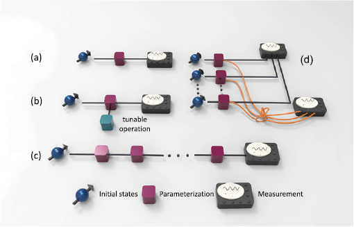
Figure 3. Schematics for basic measurement schemes in quantum metrology, including individual measurment, adaptive measurement and collective measurement.
Download figure:
Standard image High-resolution imageFor the single parameter case, a possible optimal measurement can be constructed with the eigenstates of the SLD operator. Denote  as the set of eigenstates of La, if we choose the set of POVM as the projections onto these eigenstates, then the probability for the ith measurement result is
  . In the case where
  is independent of xa, the CFI then reads

Due to the equation  , the equation above reduces to

which means the POVM  is the optimal measurement to attain the QFI. However, if the eigenstates of the SLD are dependent on xa, it is no longer the optimal measurement. In the case with a high prior information, the CFI with respect to
  (
( is the estimated value of xa) may be very close to the QFI. In practice, this measurement has to be used adaptively. Once we obtain a new estimated value
  via the measurement, we need to update the measurement with the new estimated value and then perform the next round of measurement. For a non-full rank parameterized density matrix, the SLD operator is not unique, as discussed in section 2.3.1, which means the optimal measurement constructed via the eigenbasis of SLD operator is not unique. Thus, finding a realizable and simple optimal measurement is always the core mission in quantum metrology. Update to date, only known states in single-parameter estimation that own parameter-independent optimal measurement is the so-called quantum exponential family [27, 90], which is of the form

where  is a function of the unknown parameter x,
  is a parameter-independent density matrix, and O is an unbiased observable of x, i.e.
  . For this family of states, the SLD is Lx = c(x)(O − x) and the optimal measurement is the eigenstates of O.
For multiparameter estimation, the SLD operators for different parameters may not share the same eigenbasis, which means  is no longer an optimal choice for the estimation of all unknown parameters, even with the adaptive strategy. Currently, most of the studies in multiparameter estimation focus on the construction of the optimal measurements for a pure parameterized state
  . In 2013, Humphreys et al [152] proposed a method to construct the optimal measurement, a complete set of projectors containing the operator
  (
( is the true value of
  ). Here
  equals the value of
  by taking
  . All the other projectors can be constructed via the Gram–Schmidt process. In practice, since the true value is unknown, the measurement has to be performed adaptively with the estimated values
  , similar as the single parameter case. Recently, Pezzè et al [137] provided the specific conditions this set of projectors should satisfy to be optimal, which is organized in the following three theorems.
Theorem 3.3. Consider a parameterized pure state  .
.  with
with  the true value of
  . The set of projectors
  is an optimal measurement to let the CFIM reach QFIM if and only if [137]

which is equivalent to

The proof is given in appendix I. This theorem shows that if the quantum Cramér–Rao bound can be saturated then it is always possible to construct the optimal measurement with the projection onto the probe state itself at the true value and a suitable choice of vectors on the orthogonal subspace [137].
Theorem 3.4. For a parameterized state  , the set of projectors
  is an optimal measurement to let the CFIM reach QFIM if and only if [137]

For the most general case that some projectors are vertical to  and some not, we have following theorem.
Theorem 3.5. For a parameterized pure state  , assume a set of projectors
  include two subsets
  and
and  , i.e.
  , then it is an optimal measurement to let the CFIM to reach the QFIM if and nly if [137] equation (115) is fulfilled for all the projectors in set A and (117) is fulfilled for all the projectors in set B.
Apart from the QFIM, the CFIM is also bounded by a measurement-dependent matrix with the abth entry ![$\sum\nolimits_{k}\mathrm{Re}[\mathrm{Tr}(\rho L_{a}\Pi_{k}L_{b})]$](https://content.cld.iop.org/journals/1751-8121/53/2/023001/revision2/aab5d4dieqn412.gif) [138], where
[138], where  is a set of POVM. Recently, Yang et al [138] provided the attainable conditions for the CFIM to attain this bound by generalizing the approach in [30].
3.2. Phase estimation in the Mach–Zehnder interferometer
Mach–Zehnder interferometer (MZI) is one of the most important model in quantum technology. It was first proposed in 1890th as an optical interferometer, and its quantum description was given in 1986 [139]. With the development of quantum mechanics, now it is not only a model for optical interferometer, but can also be realized via other systems like spin systems and cold atoms. The recently developed gravitational wave detector GEO 600 can also be mapped as a MZI in the absence of noise [140]. It is a little bit more complicated when the noise is involved, for which a valid bound has been provided by Branford et al [141] and is attainable by a frequency-dependent homodyne detection. Phase estimation in MZI is the earliest case showing quantum advantages in metrology. In 1981, Caves [142] showed that there exists an unused port in the MZI due to quantum mechanics and the vacuum fluctuation in that port actually affects the phase precision and limit it to the standard quantum limit (also known as shot-noise limit), which is the ultimate limit for a classical apparatus. He continued to point out that injecting a squeezed state in the unused port can lead to a high phase precision beating the standard quantum limit. This pioneer work proved that quantum technologies can be powerful in the field of precision measure, which was experimentally confirmed in [143, 144]. Since then, quantum metrology has been seeing a rapid development and grown into a major topic in quantum technology.
MZI is a two-path interferometer, which generally consists of two beam splitters and a phase shift between them, as shown in figure 4(a). In theory, the beam splitters and phase shift are unitary evolutions. A 50:50 beam splitter can be theoretically expressed by  where
where  is a Schwinger operator with
  ,
,  (
( ,
,  ) the annihilation (creation) operators for two paths. Other Schwinger operators are
  and
and  . The Schwinger operators satisfy the commutation
 ![$ \newcommand{\e}{{\rm e}} [J_{i}, J_{j}]={\rm i}\sum\nolimits_{k}\epsilon_{ijk}J_{k}$](https://content.cld.iop.org/journals/1751-8121/53/2/023001/revision2/aab5d4dieqn422.gif) with
with  the Levi-Civita symbol. The second beam splitter usually takes the form as
  . For the standard MZI, the phase shift can be modeled as
  , which means the entire operation of MZI is
  , which is a SU(2) rotation, thus, this type of MZI is also referred as SU(2) interferometer. If the input state is a pure state
  , the QFI for
  is just the variance of Jy with respect to
  , i.e.
  .
.
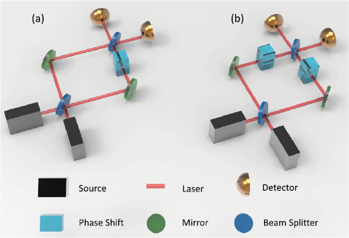
Figure 4. (a) Schematic for a standard Mach–Zehnder interferometer, which generally consists of two beam splitters and a phase shift; (b) schematic for a double phase Mach–Zehnder interferometer in which the phase shifts are put in all two paths. Here we emphasize that though the schematic is given in an optical setup, the MZI model can also be realized via other systems like spin systems and cold atoms.
Download figure:
Standard image High-resolution image3.2.1. Double-phase estimation.
A double-phase MZI consists of two beam splitters and a phase shift in each path, as shown in figure 4(b). In this setup, the operator of the two phase shifts is  . According to proposition 2.1, the QFIM for the phases is not affected by the second beam splitter
  since it is independent of the phases. Thus, the second beam splitter can be neglected for the calculation of QFIM. Now take
  and
and  as the parameters to be estimated. For a separable input state
  with
with  as a coherent state, the entries of QFIM reads [145]


Focusing on the maximization of  subject to a constraint of fixed mean photon number on b mode, Lang and Caves [145] proved that the squeezed vacuum state is the optimal choice for
  which leads to the maximum sensitivity of
  .
.
Since Caves already pointed out that the vacuum fluctuation will affect the phase sensitivity [142], it is then interesting to ask the question that how bad the phase sensitivity could be if one input port keeps vacuum? Recently Takeoka et al [146] considered this question and gave the answer by proving a no-go theorem stating that in the double phase MZI, if one input port is the vacuum state, the sensitivity can never be better than the standard quantum limit regardless of the choice of quantum state in the other port and the detection scheme. However, this theorem does not hold for a single phase shift scenario in figure 4(a). Experimentally, Polino et al [147] recently demonstrated quantum-enhanced double-phase estimation with a photonic chip.
Besides the two-phase estimation, another practical two-parameter scenario in interometry is the joint measurement of phase and phase diffusion. In 2014, Vidrighin et al [132] provide a trade-off bound on the statistical variances for the joint estimation of phase and phase diffusion. Later in 2015, Altorio et al [148] addressed the usefulness of weak measurements in this case and in 2018 Hu et al [149] discussed the SU(1,1) interferometry in the presence of phase diffusion. In the same year, Roccia et al [150] experimentally showed that some collective measurement, like Bell measurement, can benefit the joint estimation of phase and phase diffusion.
3.2.2. Multi-phase estimation.
Apart from double phase estimation, multi-phase estimation is also an important scenario in multiparameter estimation. The multi-phase estimation is usually considered in the multi-phase interferometer shown in figure 5(a). Another recent review on this topic is [16]. In this case, the total variance of all phases is the major concern, which is bounded by  according to corollary 3.1.1. For multiple phases, the probe state undergoes the parameterization, which can be represented by
  where Hj is the generator of the j th mode. In the optical scenario, this operation can be chosen as
  with
with  (aj ) as the creation (annihilation) operator for the j th mode. For a separable state
  where
where  is a state of the ith mode, and p k is the weight with p k > 0 and
  , the QFI satisfies
  [151] with
  (
( ) as the maximum (minimum) eigenvalue of Hj . From corollary 3.1.2, the total variance is then bounded by [151]
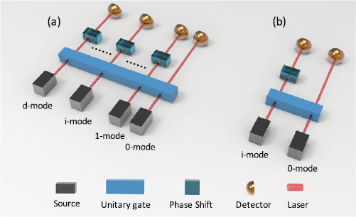
Figure 5. Schematics of (a) simultaneous multi-phase estimation and (b) independent estimation of multiple phases. 0-mode light is the reference mode. In the independent estimation, the phase in the ith mode is estimated via the MZI consisting of 0-mode and i-mode lights.
Download figure:
Standard image High-resolution imageThis bound indicates that the entanglement is crucial in the multi-phase estimation to beat the standard quantum limit.
N00N state is a well known entangled state in quantum metrology which can saturate the Heisenberg limit. In 2013, Humphreys et al [152] discussed a generalized  -mode N00N state in the form
  where
where  is the state in which only the ith mode corresponds to a Fock state and all other modes are left vacuum. c0 and c1 are real coefficients satisfying
  . The 0-mode is the reference mode and the parametrization process is
  . The generation of this state has been proposed in [153]. Since this process is unitary, the QFIM can be calculated via corollary 2.7.1 with
  . It is then easy to see that the entry of QFIM reads [152]
  , which further gives

where the optimal c1 is  .
.
Apart from the scheme in figure 5(a) with the simultaneous estimation, the multi-phase estimation can also be performed by estimating the phases independently, using the ith mode and the reference mode, as shown in figure 5(b). In this scheme, the phases are estimated one by one with the N00N state, which provides the total precision limit  [152]. Thus, the simultaneous estimation scheme in figure 5(a) shows a
  advantage compared to the independent scheme in figure 5(b). However, the performance of the simultaneous estimation may be strongly affected by the noise [154, 155] and the
  advantage may even disappear under the photon loss noise [156].
In the single phase estimation, it is known that the entangled coherent state  (
( is a coherent state and
  is the normalization) can provide a better precision limit than the N00N state [157]. Hence, it is reasonable to think the generalization of entangled coherent state may also outperform the generalized N00N state. This result was theoretically confirmed in [158]. For a generalized entangled coherent state written in the form
  with
with  , the QFIM is
 ![$\mathcal{F}_{ij}=4|c_{1}|^{2} |\alpha|^{2}[\delta_{ij}(1+|\alpha|^{2})-|c_{1}|^{2}|\alpha|^{2}]$](https://content.cld.iop.org/journals/1751-8121/53/2/023001/revision2/aab5d4dieqn466.gif) [158]. For most values of d and
[158]. For most values of d and  , the minimum
  can be written as

which is smaller than the counterpart of the generalized N00N state, indicating the performance of the generalized entangled coherent state is better than the generalized N00N state. For a large  , the total particle number ∼
 and the performances of both states basically coincide. With respect to the independent scheme, the generalized entangled coherent also shows a
  advantage in the absence of noise.
In 2017, Zhang et al [159] considered a general balanced state  with
with  . c is the normalization coefficient. Four specific balanced states: N00N state, entangled coherent state, entangled squeezed vacuum state and entangled squeezed coherent state, were calculated and they found that the entangled squeezed vacuum state shows the best performance, and the balanced type of this state outperforms the unbalanced one in some cases.
A linear network is another common structure for multi-phase estimation [160, 161]. Different with the structure in figure 5(a), a network requires the phase in each arm can be detected independently, meaning that each arm needs a reference beam. The calculation of Cramér–Rao bound in this case showed [161] that the linear network for miltiparameter metrology behaves classically even though endowed with well-distributed quantum resources. It can only achieve the Heisenberg limit when the input photons are concentrated in a small number of input modes. Moreover, the performance of a mode-separable state  may also shows a high theoretical precision limit in this case if
  .
.
Recently, Gessner [162] considered a general case for multi-phase estimation with multimode interferometers. The general Hamiltonian is  with
with  a local Hamiltonian for the ith particle in the kth mode. For the particle-separable states, the maximum QFIM is a diagonal matrix with the ith diagonal entry
  being the ith average particle number (ni is the ith particle number operator). This bound could be treated as the shot-noise limit for the multi-phase estimation. For the mode-separable states, the maximum QFIM is also diagonal, with the ith entry
  , which means the maximum QFIM for mode-separable state is larger than the particle-separate counterpart. Taking into account both the particle and mode entanglement, the maximum QFIM is in the form
  , which gives the Heisenberg limit in this case.
The comparison among the performances of different strategies usually requires the same amount of resources, like the same sensing time, same particle number and so on. Generally speaking, the particle number here usually refers to the average particle number, which is also used to define the standard quantum limit and Heisenberg limit in quantum optical metrology. Although the Heisenberg limit is usually treated as a scaling behavior, people still attempt to redefine it as an ultimate bound given via quantum mechanics by using the expectation of the square of number operator to replace the square of average particle number [163], i.e. the variance should be involved in the Heisenberg limit [163, 164] and be treated as a resource.
3.3. Waveform estimation
In many practical problems, like the detection of gravitational waves [141] or the force detection [165], what needs to be estimated is not a parameter, but a time-varing signal. The QFIM also plays an important role in the estimation of such signals, also known as waveform estimation [166]. By discretizing time into small enough intervals, the estimation of a time-continuous signal  becomes the estimation of multiparameters xj 's. The prior information of the waveform has to be taken into account in the estimation problem, e.g. restricting the signal to a finite bandwidth, in order to make the estimation error well-defined. The estimation-error covariance matrix
  is then given by

where  and y denotes the measurement outcome. Tsang proved the most general form of Bayesian quantum Cramér-Rao bound

where the classical part

depends only on the prior information about the vector parameter  and the quantum part [29, 166]

depends on the parametric family  of density operators with
  being determined via

Note that  is an extended version of SLD and is not necessary to be Hermitian. When all
  's are Hermitian,
  is the average of the QFIM over the prior distribution of
  .
.  can also be anti-Hermiaition [29]. In this case, the corresponding bound is equivalent to the SLD one for pure states but a potentially looser one for mixed states. For a unitary evolution, the entire operator U can be discretized into
  , where
  . Denote
  and
and  with
with  the probe state, the quantum part in equation (127) reads [166]

Taking the continuous-time limit, it can be rewritten as [166]

Together with  , the fundamental quantum limit to waveform estimation based on QFIM is established [166]. The waveform estimation can also be solved with other tools, like the Bell–Ziv–Zakai lower bounds [167].
3.4. Control-enhanced multiparameter estimation
The dynamics of many artificial quantum systems, like the Nitrogen-vacancy center, trapped ion and superconducting circuits, can be precisely altered by control. Hence, control provides another freedom for the enhancement of the precision limit in these apparatuses. It is already known that quantum control can help to improve the QFI to the Heisenberg scaling with the absence of noise in some scenarios [54, 169–170]. However, like other resources, this improvement could be sensitive to the noise, and the performance of optimal control may strongly depend on the type of noise [171, 172]. In general, the master equation for a noisy quantum system is described by

Here  is a
is a  -dependent superoperator. For the Hamiltonian estimation under control, the dynamics is

where  is the control Hamiltonian with Hk the kth control and
  the corresponding time-dependent control amplitude. For a general Hamiltonian, the optimal control can only be tackled via numerical methods. One choice for this problem is the Gradient ascent pulse engineering algorithm.
Gradient ascent pulse engineering (GRAPE) algorithm is a gradient-based algorithm, which was originally developed to search the optimal control for the design of nuclear magnetic resonance pulse sequences [173], and now is extended to the scenario of quantum parameter estimation [171, 172]. As a gradient-based method, GRAPE requires an objective function and analytical expression of the corresponding gradient. For quantum single-parameter estimation, the QFI is a natural choice for the objective function. Of course, in some specific systems the measurement methods might be very limited, which indicates the CFI is a proper objective function in such cases. For quantum multiparameter estimation, especially those with a large parameter number, it is difficult or even impossible to take into account the error of every parameter, and thus the total variance  which represents the average error of all parameters, is then a good index to show system precision. According to corollary 3.1.1,
  and
and  (for fixed measurement) could be proper objective functions for GRAPE if we are only concern with the total variance. For two-parameter estimation,
  and
and  reduce to the effective QFI
  and CFI
  according to corollary 3.1.3. However, as the parameter number increases, the inverse matrix of QFIM and CFIM are difficult to obtain analytically, and consequently superseded objective functions are required.
  or
or  , based on corollary 3.1.2, is then a possible superseded objective function for fixed measurement. However, the use of
  should be very cautious since
  cannot always be achievable. The specific expressions of gradients for these objective functions in Hamiltonian estimation are given in appendix J.
The flow of the algorithm, shown in figure 6, is formulated as follows [171, 172]:
- (i)Guess a set of initial values for ( is the kth control at the j th time step).
- (ii)Evolve the dynamics with the controls.
- (iii)Calculate the objective function. For single-parameter estimation, the objective function can be chosen as QFI or CFI (for mixed measurement). For two-parameter estimation, it can be chosen as or . For large parameter number, it can be chosen as or .
- (iv)Calculate the gradient.
- (v)Update to ( is a small quantity) for all j simultaneously.
- (vi)Go back to step (ii) until the objective function converges.


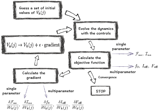
Figure 6. Flow chart of GRAPE algorithm for controlled single-parameter and multiparameter estimation. Reprinted figure with permission from [171, 172]. Copyright (2019) by the American Physical Society.
Download figure:
Standard image High-resolution imageIn step (v), all  are updated simultaneously in each time of iteration [173], as shown in figure 7(a), which could improve the speed of convergence in some cases. However, this parallel update method does not promise the monotonicity of convergence, and the choice of initial guess of
  is then important for a convergent result. The specific codes for this algorithm can be found in the package QuanEstimation14.

Figure 7. (a) In GRAPE, the entire evolution time T is cut into m parts with time interval  , i.e.
  .
.  within the j th time interval is denoted as
  and is assumed to be a constant. All the
  are simultaneously updated in each iteration. (b) Krotov's method updates one
  in each iteration.
Download figure:
Standard image High-resolution imageKrotov's method is another gradient-based method in quantum control, which promises the monotonicity of convergence during the iteration [174]. Different from GRAPE, only one  is updated in each iteration in Krotov's method, as shown in figure 7(b). This method can also be extended to quantum parameter estimation with the aim of searching the optimal control for a high precision limit. It is known that the gradient-based methods can only harvest the local extremals. Thus, it is also useful to involve gradient-free methods, including Monte Carlo method and particle swarm optimization, into the quantum parameter estimation, or apply a hybrid method combining gradient-based and gradient-free methods as discussed in [175].
3.5. Estimation of a magnetic field
Measurement of the magnetic fields is an important application of quantum metrology, as it promises better performances than the classical counterparts. Various physical systems have been used as quantum magnetometers, including but not limited to nitrogen-vacancy centers [176, 177], optomechanical systems [178], and cold atoms [179].
A magnetic field can be represented as a vector,  , in the spherical coordinates, where B is the amplitude, and
  define the direction of the field. Therefore, the estimation of a magentic field is in general a three-parameter estimation problem. The estimation of the amplitude with known angles is the most widely-studied case in quantum metrology, both in theory and experiments. For many quantum systems, it is related to the estimation of the strength of system-field coupling. In the case where one angle, for example
  is known, the estimation of the field becomes a two-parameter estimation problem. The simplest quantum detector for this case is a single-spin system [48, 53]. An example of the interaction Hamiltonian is
  with
with  and
and  . The QFIM can then be obtained by making use of the expressions of
  operators [48, 53]

where  . The entries of QFIM then read


where  is the Bloch vector of the probe state. The maximal values of
  and
and  can be attained when
  is vertical to both
  and
and  . However, as a two-parameter estimation problem, we have to check the value of
 ![$\langle\psi_{0}|[\mathcal{H}_{B},\mathcal{H}_{\theta}]|\psi_{0}\rangle$](https://content.cld.iop.org/journals/1751-8121/53/2/023001/revision2/aab5d4dieqn547.gif) due to corollary 3.2.2. Specifically, for a pure probe state it reads
due to corollary 3.2.2. Specifically, for a pure probe state it reads ![$\langle\psi_{0}|[\mathcal{H}_{B},\mathcal{H}_{\theta}]|\psi_{0}\rangle =-\sin(Bt)(\vec {n}_{0}\times\vec {n}_{1})\cdot\vec {\sigma}$](https://content.cld.iop.org/journals/1751-8121/53/2/023001/revision2/aab5d4dieqn548.gif) . For the time
. For the time  (
( ), the expression above vanishes. However, another consequence of this condition is that
  also vanishes. Thus, single-qubit probe may not be an ideal magnetometer when at least one angle is unknown. One possible candidate is a collective spin system, in which the
  operator and QFIM are provided in [180]. Another simple and practical-friendly candidate is a two-qubit system. One qubit is the probe and the other one is an ancilla, which does not interact with the field. Consider the Hamiltonian
  , the maximal QFIM in this case is (in the basis
  ) [84]
which can be attained by any maximally entangled state and the Bell measurement as the optimal measurement. With the assistance of an ancilla, all three parameters  of the field can be simultaneously estimated. However,
  and
and  are only proportional to
  , indicating that unlike the estimation of the amplitude, a longer evolution time does not always lead to a better precision for the estimation of
  or
or  .
.
In 2016, Baumgratz and Datta [181] provided a framework for the estimation of a multidimensional field with noncommuting unitary generators. Analogous to the optical multi-phase estimation, simultaneous estimation shows a better performance than separate and individual estimation.
To improve the performance of the probe system, additional control could be employed. For unitary evolution [84], showed that the performance can be significantly enhanced by inserting the anti-evolution operator as the control. Specifically if after each evolution of a period of  , we insert a control which reverses the evolution as
  , the QFIM can reach
where N is the number of the injected control pulses, and  . In practice the control needs to be applied adaptively as
  with
with  as the estimated value obtained from previous measurement results. In the controlled scheme, the number of control pulses becomes a resource for the estimation of all three parameters. For the amplitude, the precision limit is the same as non-controlled scheme. But for the angles, the precision limit is significantly improved, especially when N is large. When
  , the QFIM becomes
which reaches the highest precision for the estimation of B,  and
and  simultaneously. Recently, Hou et al [182] demonstrated this scheme up to eight controls in an optical platform and demonstrate a precision near the Heisenberg limit.
Taking into account the effect of noise, the optimal control for the estimation of the magnetic field is then hard to obtain analytically. The aforementioned numerical methods like GRAPE or Krotov's method could be used in this case to find the optimal control. The performance of the controlled scheme relies on the specific form of noise [171, 172], which could be different for different magnetometers.
In practice, the magnetic field may not be a constant field in space. In this case, the gradient of the field also needs to be estimated. The corresponding theory for the estimation of gradients based on Cramér–Rao bound has been established in [183, 184].
3.6. Other applications and alternative mathematical tools
Apart from the aforementioned cases, quantum multiparameter estimation is also studied in other scenarios, including the spinor systems [186], unitary photonic systems [187], networked quantum sensors [188], and the quantum thermometry [189]. In the case of noise estimation, the simultaneous estimation of loss parameters has been studied in [190].
In 2016, Tsang et al [191] used quantum multiparameter estimation for a quantum theory of superresolution for two incoherent optical point sources. With weak-source approximation, the density operator for the optical field in the imaging plane can be expressed as  , with
  the average photon number in a temporal mode,
  the vacuum state,
  the quantum state of an arrival photon from the point source located at xj of the object plane,
  the wave function in the image plane, and
  the photon image-plane position eigenstate. Taking the position coordinates to be one-dimensional, the parameters to be estimated are x1 and x2. The performance of the underlying quantum measurement can be assessed by the CFIM and its fundamental quantum limit can be revealed by the QFIM. In this case, the QFIM is analytically calculated in the 4-dimensional Hilbert subspace spanned by
  ,
,  ,
,  , and
, and  . For convenience, the two parameters x1 and x2 can be transformed to the centriod
  and the separation
  . Assuming the imaging system is spatially invariant such that the point-spread function of the form
  with real-valued
  , the QFIM with respect to
  and
and  is then given by

where ![$\Delta k^2 = \int_{-\infty}^\infty [\partial \psi(y) / \partial y]^2\,\mathrm{d}y$](https://content.cld.iop.org/journals/1751-8121/53/2/023001/revision2/aab5d4dieqn585.gif) and
and  [191]. With this result, it has been shown that direct imaging performs poorly for estimating small separations and other elaborate methods like spatial-mode demultiplexing and image inversion interferometry can be used to achieve the quantum limit [191, 192].
The design of enhanced schemes for quantum parameter estimation would inevitably face optimization processes, including the optimization of probe states, the parameterization trajectories, the measurement and so on. If control is involved, one would also need to harvest the optimal control. Therefore, the stochastic optimization methods, including convex optimization, Monte Carlo method and machine learning, could be used in quantum parameter estimation.
Machine learning is one of the most promising and cutting-edge methods nowadays. In recent years, it has been applied to condensed matter physics for phase transitions [193, 194], design of a magneto-optical trap [195] and other aspects [196]. With respect to quantum parameter estimation, in 2010, Hentschel and Sanders [197] applied the particle swarm optimization algorithm [198] in the adaptive phase estimation to determine the best estimation strategy, which was experimentally realized by Lumino et al [199] in 2018. Meanwhile, in 2017, Greplova et al [200] proposed to use neural networks to estimate the rates of coherent and incoherent processes in quantum systems with continuous measurement records. In the case of designing controlled schemes, similar to gradient-based methods, machine learning could also help use to find the optimal control protocal in order to achieve the best precision limit [185]. In particular, for quantum multiparameter estimation, there still lacks of systematic research on the role of machine learning. For instance, we are not assured if there exists different performance compared to single-parameter estimation.
As a mathematical tool, quantum Cramér–Rao bound is not the only one for quantum multiparameter estimation. Bayesian approach [203–207], including Ziv–Zakai family [167, 168, 201] and Weiss–Weinstein family [166, 208], and some other tools [208–210] like Holevo bound [2, 28, 202], have also shown their validity in various multiparameter scenarios. These tools beyond the Cramér–Rao bound will be thoroughly reviewed by Guţă et al [211] in the same special issue and hence we do not discuss them in this paper. Please see [211] for further reading of this topic. In some scenarios in quantum parameter estimations, there may exist some parameters that not of interest but affect the precision of estimating other parameters of interest, which is usually referred to as the nuisance parameters. Suzuki et al [212] has thoroughly reviewed the quantum state estimation with nuisance parameters in the same special issue. Please see [212] for further reading.
4. Conclusion and outlook
Quantum metrology has been recognized as one of the most promising quantum technologies and has seen a rapid development in the past few decades. Quantum Cramér–Rao bound is the most studied mathematical tool for quantum parameter estimation, and as the core quantity of quantum Cramér–Rao bound, the QFIM has drawn plenty of attentions. It is now well-known that the QFIM is not only a quantity to quantify the precision limit, but also closely connected to many different subjects in quantum physics. This makes it an important and fundamental concept in quantum mechanics.
In recent years, many quantum multiparameter estimation schemes have been proposed and discussed with regard to various quantum systems, and some of them have shown theoretical advances compared to single-parameter schemes. However, there are still many open problems, such as the design of optimal measurement, especially simple and practical measurement which are independent of the unknown parameters, as well as the robustness of precision limit against the noises and imperfect controls. We believe that some of the issues will be solved in the near future. Furthermore, quantum multiparameter metrology will then go deeply into the field of applied science and become a basic technology for other aspects of sciences.
Acknowledgments
The authors thank Zibo Miao, Christiane Koch, Rafał Demkowicz-Dobrzański, Yanming Che, Dominic Branford, Dominik Šafránek, Jasminder Sidhu, Wenchao Ge, Jesus Rubio, Wojciech Rzadkowski, Marco Genoni, Haggai Landa and two anonymous referees for for helpful discussions and suggestions. JL particularly thanks Yanyan Shao and Jinfeng Qin for the assistance on drawing some of the schematics. JL acknowledges the support from National Natural Science Foundation of China (Grant No. 11805073) and the startup grant of HUST. HY acknowledges the support from the Research Grants Council of Hong Kong (GRF No. 14207717). XML acknowledges the support from the National Natural Science Foundation of China (Grant Nos. 61871162 and 11805048), and Zhejiang Provincial Natural Science Foundation of China (Grant No. LY18A050003). XW acknowledges the support from National Key Research and Development Program of China (Grant Nos. 2017YFA0304202 and 2017YFA0205700), the National Natural Science Foundation of China (Grant Nos. 11935012 and 11875231), and the Fundamental Research Funds for the Central Universities (Grant No. 2017FZA3005).
Appendix A. Derivation of traditional form of QFIM
The traditional calculation of QFIM usually assume a full rank density matrix, of which the spectral decompostion is in the form
where  and
and  are ith eigenvalue and eigenstate of
  .
.  is the dimension of
  .
.  satisfies
  with
with  the identity matrix. Substituting equation (A.1) into the equation of SLD (
 is the abbreviation of
  )
)

and taking  on both sides of above equation, one can obtain

Next, utlizing equation (A.1), the QFIM

can be rewritten as

Inserting the equation  into above equation, one can obtain
Substituting equation (A.3) into this equation, one has
Exchange subscripts i and j , the traditional form of QFIM is obtained as below
Appendix B. Derivation of QFIM for arbitrary-rank density matrices
In this appendix we show the detailed derivation of QFIM for arbitrary-rank density matrices. Here the spectral decompostion of  is
is

where  and
and  are ith eigenvalue and eigenstate of
  . Notice N here is the dimension of
  's support. For a full-rank density matrix, N equals to
  , the dimension of
  , and for a non-full rank density matrix,
  , and
, and  (
( is the identity matrix and
  ). Furthermore,
  for
for ![$i\in[0,N-1]$](https://content.cld.iop.org/journals/1751-8121/53/2/023001/revision2/aab5d4dieqn611.gif) . With these notations,
. With these notations,  can be expressed by
Followings are the detailed proof of this equation.
Based on the equation of SLD ( is the abbreviation of
  )
)

one can easily obtain

The derivative of  reads
reads  , which gives
 is the Kronecker delta function (
 for i = j and zero otherwise). Substituting this expression into above equation,
  can be calculated as

With the solution of SLD, we can now further calculate the QFIM. Utlizing equation (B.1), the QFIM can be rewritten into

Inserting the equation  into above equation, one can obtain
In this equation, it can be seen that the arbitrary part of  does not affect the value of QFIM since it is not involved in above equation, but it provides a freedom for the optimal measurements, which will be further discussed later. Substituting equation (B.5) into above equation, we have
where the fact  has been applied. The third term in above equation can be further calculated as
Therefore equation (B.8) can be rewritten into
Exchange the subscripts i and j in the second and fourth terms of above equation, it reduces into a symmetric form as shown in equation (B.2).
Appendix C. QFIM in Bloch representation
Bloch representation is a well-used representation of quantum states in quantum mechanics and quantum information theory. For a d-dimensional quantum state  , it can be expressed by

where  is the Bloch vector (
 ) and
) and  is a (d2 − 1)-dimensional vector of
  generator satisfying
  and
and
where  is the Kronecker delta function.
  and
and  are the symmetric and antisymmetric structure constants, which can be calculated via the following equations


It is easy to find  and
and  keeps still for any order of ijl, which will be used in the following.
Now we express the SLD operator with the  generators as [43, 44]

where za is a number and  is a vector. In the following we only use z and
  for convenience. From the equation
  , one can find

where  . Furthermore,

The coefficients of  in equation (C.7) from both sides have to be the same, which gives

which can also be obtained from the equation  . Similarly, the coefficients of
  in equation (C.7) from both sides have to be the same, which gives

This can also be obtained by multipling  on both sides of equation (C.7) and then taking the trace. Now we introduce the matrix G with the entry

It is easy to see G is real symmetric. Substituting equation (C.2) into the equation above, it can be further written into

Hence, the last term in equation (C.10) can be rewritten into
Substituting this equation into equation (C.10), one has  , which immediately leads to

Futhermore, one can check that

Utilizing this equation, equation (C.14) reduces to

Therefore,

Next, we calculate the entry of QFIM and we will use the full notation za and  instead of z,
  . The entry of QFIM reads
Based on equations (C.9) and (C.14), one can obtain

Hence, the QFIM can be written as

Utilizing equation (C.17), the QFIM can be finally written into
The theorem has been proved.
The simplest case here is single-qubit systems. The corresponding density matrix is  with
with  the vector of Pauli matrices and
  is the 2 by 2 identity matrix. In this case,
  (
( is the 3 by 3 identity matrix) due to the fact
  . Equation (C.21) then reduces to

It can be checked that

The QFIM then reads

or equivalently,

Appendix D. One-qubit basis-independent expression of QFIM
This appendix shows the proof of theorem 2.6. We first prove that the QFIM for one-qubit mixed state can be written as [46]

Utilizing the spectral decomposition  , the first term reads
The second term
Since
and
one can finally obtain
which coincides with the traditional formula of QFIM in theorem 2.1. Equation (D.1) is then proved. Furthermore, one may notice that  ,
,  , and
, and  , which gives
namely, the equality ![$\mathrm{Tr}\left[(\partial_{x_{a}}\rho)(\partial_{x_{b}}\rho)\right]=\mathrm{Tr} \left(\rho\{\partial_{x_{a}}\rho, \partial_{x_{b}}\rho)\}\right)$](https://content.cld.iop.org/journals/1751-8121/53/2/023001/revision2/aab5d4dieqn657.gif) holds for single-qubit mixed states. Thus, equation (D.1) can further reduce to
holds for single-qubit mixed states. Thus, equation (D.1) can further reduce to

The theorem has been proved.
Appendix E. Derivation of SLD operator for Gaussian states
E.1. SLD operator for multimode Gaussian states
The derivation in this appendix is majorly based on the calculation in [62, 67]. Let us first recall the notations before the derivation. The vector of quadrature operators are defined as  .
.  is a symplectic matrix
  .
.  is the characteristic function. Furthermore, denote
  . To keep the calculation neat, we use
  ,
,  , L instead of
  ,
,  ,
,  in this appendix. Some other notations are
  and
and  .
.
The characteristic function  , where
  with
with  . Substituting D into the equation
  and taking the trace, we obtain

Next, assume the SLD operator is in the following form

where L(0) is a real number,  is a 2m-dimensional real vector and G is a 2m-dimensional real symmetric matrix. These conditions promise the Hermiticity of SLD. With this ansatz, equation (E.1) can then be rewritten into

Now we calculate  in equation (E.3). Denote
 ![$[A,\cdot]=A^{\times}(\cdot)$](https://content.cld.iop.org/journals/1751-8121/53/2/023001/revision2/aab5d4dieqn676.gif) , one can have
, one can have
where we have used the fact  and
and  which come from the equation
  . Substituting the equation

into the first line of equation (E.4) and repeat the calculation, one can obtain  . Combining this equation with equation (E.4),
  can be finally written as

which further gives  . Based on this equation, it can be found
  . Again since
  , it reduces to

Next, continue to take the derivative on  , we have

Due to the Baker–Campbell–Hausdorff formula, ![$ \newcommand{\re}{{\rm Re}} \renewcommand{\dag}{\dagger}D^{\dagger}R_{i}D=R_{i} +[-{\rm i} \vec {R}^{\mathrm{T}}\Omega\vec {s},R_{i}]=R_{i}+s_{i}$](https://content.cld.iop.org/journals/1751-8121/53/2/023001/revision2/aab5d4dieqn686.gif) , the commutation between Ri and D can be obtained as
, the commutation between Ri and D can be obtained as ![$[R_{i},D]=s_{i}D$](https://content.cld.iop.org/journals/1751-8121/53/2/023001/revision2/aab5d4dieqn687.gif) , which further gives
, which further gives  . Then equation (E.8) can be rewritten into

And one can finally obtain
With equations (E.7) and (E.10), equation (E.3) can be expressed by
On the other hand, from the expression of characteristic function

it can be found that

and
Then we have  , and
, and
Substituting these equations into equation (E.11),  can be expressed by
This equation can be written into a more compact way as below
Compare this equation with equation (E.13), it can be found that


From the second equation above, one can obtain

Using this equation and the equation (E.16), it can be found that

Once we obtain the expression of G, L(0) and  can be obtained correspondingly, which means we need to solve equation (E.18), which can be rewritten into following form

Since  and
and  , above equation can be rewritten into

where  . Denote the map
  , then
  . The map
  can be decomposed via the generators
  (
( ), where

for 
 is a 2m-dimensional matrix with all the entries zero expect the
  block shown as below
where  represents a 2 by 2 block with zero entries.
  is similar to
  but replace the block
  with
with  .
.  satisfies the orthogonal relation
  . Recall that
  , it is easy to check that


Next decompose  with
with  as
as

where ![$g^{(\,jk)}_{l}=\mathrm{Tr}[S^{-1}\dot{C}(S^{\mathrm{T}}){}^{-1}A^{(\,jk)}_{l}]$](https://content.cld.iop.org/journals/1751-8121/53/2/023001/revision2/aab5d4dieqn713.gif) . Decomposing
. Decomposing  as
as  , and substituting it into equation (E.22), we have

Utilizing equations (E.25) and (E.26), above equation reduces to

which indicates

Thus,  can be solved as below
In summary, the SLD can be expressed by

where
with

for  and
and ![$g^{(\,jk)}_{l}=\mathrm{Tr}[S^{-1}\dot{C}(S^{\mathrm{T}}){}^{-1}A^{(\,jk)}_{l}]$](https://content.cld.iop.org/journals/1751-8121/53/2/023001/revision2/aab5d4dieqn718.gif) . And
. And


E.2. SLD operator for single-mode Gaussian state
For a single-mode case, a 2 by 2 symplectic S matrix satisfies  . Based on the equation
  (c is the symplectic value), the following equations can be obtained


Together with the equation  , the symplectic value c can be solved as
  . Assume the form


Substituting above expressions into equation (E.37), it can be found  need to satisfy

Since there is only four constrains for these five variables, one of them is free. We take  , and the symplectic matrix reduces to

where  satisfies
  and
and  . Based on theorem 2.9, we obtain


where  ,
,  are short for
  and
and  . Meanwhile, we have


These expressions immediately give  as below
Define a matrix

![$[G_{x_a}]_{00}$](https://content.cld.iop.org/journals/1751-8121/53/2/023001/revision2/aab5d4dieqn733.gif) can be rewritten into
can be rewritten into

Similarly, one can obtain

and

These expressions indicate

with

Appendix F. QFIM and Bures metric
The Bures distance between two quantum states  and
and  is defined as

where  is the quantum fidelity. Now we calcuate the fidelity for two close quantum states
  and
and  . The Taylor series of
  (up to the second order) reads

In the following  will be used as the abbreviation of
  . Utilizing the equation above, one can obtain
Now we assume

Taking the square of above equation and compare it to equation (F.3), one can obtain


where  is short for
  .
.  (not
(not  ) is used to make sure the equation is unchanged when the subscripts a and b exchange. Meawhile, from equation (F.4), the Bures metric
  (the abbreviation
  will bu used below) can be calculated as

As long as we obtain the specific expressions of Wa and Yab from equations (F.5) and (F.6),  can be obtained immediately. To do that, we utilize the spectral decomposition
  . In the basis
  , the matrix entries (
![$[\cdot]_{ij}=\langle\lambda_{i} |\cdot|\lambda_{j}\rangle$](https://content.cld.iop.org/journals/1751-8121/53/2/023001/revision2/aab5d4dieqn751.gif) ) read
) read


Here ![$[\partial_{x_{a}}\rho]_{ij}=\delta_{ij}\partial_{x_{a}} \lambda_{i}-(\lambda_{i}-\lambda_{j})\langle\lambda_{i}|\partial_{x_{a}}\lambda_{j}\rangle$](https://content.cld.iop.org/journals/1751-8121/53/2/023001/revision2/aab5d4dieqn752.gif) , and
, and
where  and
and  are short for
  and
and  . Now we denote
  's dimension as N and
  for
for  . Under the assumption that the support
  is not affected by the values of
  , i.e. the rank of
  equals to that of
  ,
,  and
and  are both block diagonal. Based on equation (F.5), the ijth matrix entry of Wa can be calculated as

for ![$i,j\in [0,M-1]$](https://content.cld.iop.org/journals/1751-8121/53/2/023001/revision2/aab5d4dieqn766.gif) and
and ![$[W_{a}]_{ij}=0$](https://content.cld.iop.org/journals/1751-8121/53/2/023001/revision2/aab5d4dieqn767.gif) for others. One can observe that Wa is a Hermitian matrix, and
for others. One can observe that Wa is a Hermitian matrix, and

which means there is no first order term in Bures metric. With respect to the second order term, we need to know the value of ![$[Y_{ab}]_{ii}$](https://content.cld.iop.org/journals/1751-8121/53/2/023001/revision2/aab5d4dieqn768.gif) . From equation (F.6), one can obtain
. From equation (F.6), one can obtain

Due to the fact  , one can have

which further gives
where the fact  has been applied. Next, from equation (F.11) one can obtain

which means
Thus,  can then be expressed by
With this equation, we finally obtain

One should notice that this proof shows that this relation is established for density matrices with any rank as long as the rank of  is unchanged with the varying of
  . In the case the rank can change, a thorough discussion can be found in [87].
Appendix G. Relation between QFIM and cross-correlation functions
This appendix gives the thorough calculation of the relation between QFIM and dynamic susceptibility in [109]. Consider the unitary parameterization  with a thermal state
  . Here
  is the partition function. Oa is a Hermitian generator for xa. In the following we set kB = 1 and assume all Oa are commutative, i.e.
 ![$[O_{a},O_{b}]=0$](https://content.cld.iop.org/journals/1751-8121/53/2/023001/revision2/aab5d4dieqn777.gif) for any a and b. Denote
for any a and b. Denote  , and
, and  , the symmetric cross-correlation spectrum in this case reads

Utilizing the energy basis  (with Ei the ith energy), it can be rewritten into

Further use the equation  ,
,  can reduce to

With this expression, one can find
Since
one can obtain

From the expression of QFIM, it can be found that

It can also be checked that

In the mean time, the asymmetric cross-correlation spectrum is in the form
which directly gives the relation between  and Sab as below
namely,

which is just the fluctuation-dissipation theorem. Using this relation, one can further obtain the result in [109] as below

Appendix H. Derivation of quantum multiparameter Cramér–Rao bound
The derivation of quantum multiparameter Cramér–Rao bound is based on the Cauchy–Schwarz inequality below

which comes from the complete form

Define X and Y as


where  are real numbers for any m, and
  . Here Om is an observable defined as

 is the estimator of xm and is the function of kth result. Based on equation (H.3), it can be calculated that
  , which can be symmetrized into
  . Define
  ,
,  can be further rewritten into

Similarly, define  and through some algebra,
  can be calculated as

where C is the covariance matrix for {Om}, and is defined as  . Furthermore, one can also obtain

where the entry of B is defined as  . Utilizing
  , Bml reduces to
  . Since we consider unbiased estimators, i.e.
  , Bml further reduces to
  , with
  the Kronecker delta function. Hence, for unbiased estimators B is actually the identity matrix
  .
.
Now substituting equations (H.6)–(H.8) into the Cauchy–Schwarz inequality (H.1), one can obtain

Assuming  is invertable, i.e. it is positive-definite, and taking
  , above inequality reduces to
  . Since
  is positive-definite,
  is also positive-definite, which means
  is a positive number, thus, the above equation can further reduce to
  , namely,

Next we discuss the relation between C and  . Utilizing the defintion of Om, Cml can be written as
and  for unbiased estimators reads

If  is a set of projection operators, it satisfies
  . For unbiased estimators,
  , which gives
  , i.e.

If  is a set of POVM, one can see
In the mean time,

Now define  . Based on the Cauchy–Schwarz inequality
  , which is valid for any operator A, one can immediately obtain
  , which further gives
  . Through some calculations, the expression of
  is in the form
Now taking the difference of equations (H.14) and (H.15), it can be found

Finally, we obtain the following inequality  , namely, for any POVM measurement,

Based on inequality (H.10) and the property of quadratic form, we finally obtain  . Consider the repetition of experiments (denoted as n), above bound needs to add a factor of 1/n. Hence the quantum multiparameter Cramér–Rao bound can be finally expressed by

Appendix I. Construction of optimal measurement for pure states
Assume the true values of the vector of unknown parameters  is
is  , we now provide the proof that for a pure parameterized state
  , a set of projectors containing the state
  , i.e.
  is possible to be an optimal measurement to attain the quantum Cramér–Rao bound, as shown in [137, 152]. The calculation in this appendix basically coincides with the appendix in [137].
Since  contains the information of the true value, in practice one need to use the estimated value of
  (denoted as
  ) to construct
  to perform this measurement, then improve the accuracy of
  adaptively. Thus, it is reasonable to assume
  . The probability for
  is
is  , which gives the CFIM as below

At the limit  , it is

For the k = 0 term,
and  . Thus, the CFIM is

Due to the fact
one can have

where
To let  , Q has to be a zero matrix. Since the diagonal entry

in which all the terms within the summation are non-negative. Therefore, its value is zero if and only if

Furthermore, this condition simultaneously makes the non-diagonal entries of Q vanish. Thus, it is the necessary and sufficient condition for Q = 0, which means it is also the necessary and sufficient condition for  at the point of true value. One may notice that the limitation in equation (I.9) is a 0/0 type. Thus, we use the formula
  to further calculate above equation. With this formula, one has

 cannot generally be zero for all xj since all
  are not orthogonal in general. Thus, equation (I.9) is equivalent to

Appendix J. Gradient in GRAPE for Hamiltonian estimation
J.1. Gradient of CFIM
The core of GRAPE algorithm is to obtain the expression of gradient. The dynamics of the system is described by

For the Hamiltonian estimation under control, the dynamics is

where  is the control Hamiltonian with Hk the kth control and
  the corresponding time-dependent control amplitude. To perform the algorithm, the entire evolution time T is cut into m parts with time interval
  , i.e.
  .
.  within the j th time interval is denoted as
  and is assumed to be a constant.
For a set of probability distribution  with
with  a set of POVM. The gradient of
  at target time T reads [172]
where


and  ,
,  and
and  are Hermitian operators and can be expressed by


The notation ![$A^{\times}(\cdot):=[A,\cdot]$](https://content.cld.iop.org/journals/1751-8121/53/2/023001/revision2/aab5d4dieqn854.gif) is a superoperator.
is a superoperator.  is the Kronecker delta function.
  is the propagating superoperator from the j th time point to the
  th time with the definition
  for
for  . We define
  for
for  .
.  is the quantum state at j th time.
For a two-parameter case  , the objective function can be chosen as
  according to corollary 3.1.3, and the corresponding gradient is
For the objective function
the gradient reads

J.2. Gradient of QFIM
Now we calculate the gradient of the QFIM. Based on the equation

we can obtain

Similarly, we have
Next, from the definition of QFIM, the gradient for  at target time T reads [172]
Combing equations (J.13)–(J.15), one can obtain
Substituing the specific expressions of  given in [172], one can obtain the gradient of
  as below
The gradient for the diagonal entry  reduces to the form in [172], i.e.

Footnotes
- 6
In the entire paper the notation
() is used as an abbreviation of . - 7 represents the set of real numbers.
- 8
The derivation is in appendix B.
- 9
The derivation of this theorem is in appendix E.1.
- 10
The derivation of this corollary is in appendix E.2.
- 11
The derivation is given in appendix F.
- 12
The details of the derivation can be found in appendix G.
- 13
The derivation of this theorem is given in appendix H.
- 14
QuanEstimation package: https://github.com/LiuJPhys/QuanEstimation.


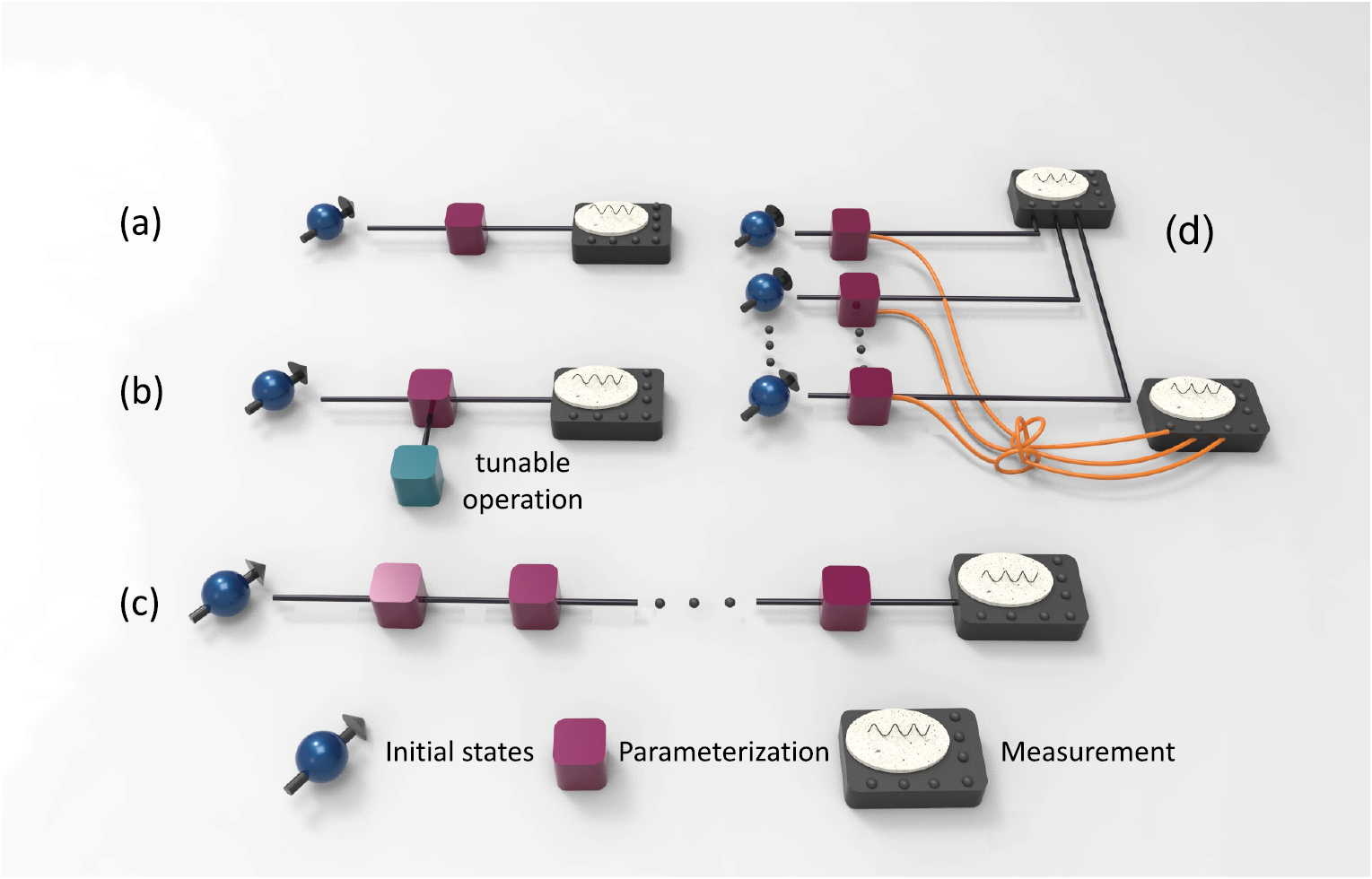