

Abstract
Lossy bosonic channels play an important role in a number of quantum information tasks, since they well approximate thermal dissipation in an experiment. Here, we characterize their metrological power in the idler-free and entanglement-assisted cases, using respectively single- and two-mode Gaussian states as probes. In the problem of estimating the loss parameter, we study the power-constrained quantum Fisher information (QFI) for generic temperature and loss parameter regimes, showing qualitative behaviours of the optimal probes. We show semi-analytically that the two-mode squeezed-vacuum state optimizes the QFI for any value of the loss parameter and temperature. We discuss the optimization of the total QFI, where the number of probes is allowed to vary by keeping the total power constrained. In this context, we elucidate the role of the 'shadow-effect', or passive signature, for reaching a quantum advantage. Finally, we discuss the implications of our results for the quantum illumination and quantum reading protocols.
Export citation and abstract BibTeX RIS

Original content from this work may be used under the terms of the Creative Commons Attribution 4.0 licence. Any further distribution of this work must maintain attribution to the author(s) and the title of the work, journal citation and DOI.
1. Introduction
Lossy channels are important to describe realistic scenarios in all quantum information tasks. Key examples are given by dissipative bosonic channels [1]. Assume a bosonic mode interacting with a thermal bath at a certain temperature. How is the quantum state susceptible to the presence of the bath? In other words, how well can we estimate the amount of losses given a certain probe? This question, aside being interesting for calibrating a number of physical setups, is important for several imaging [2–5], detection [6–12], and communication [13–18] scenarios. Quantum information tools based on the quantum Fisher information (QFI) have been developed in a generic quantum parameter estimation framework [19, 20]. Mostly, one aims to answer questions about optimality of the input state and the measurement. This is indeed challenging when the dynamics are non-unitary, because the procedure involves computing distances and/or fidelities between mixed quantum states. However, the single loss parameter case is 'simple' enough to be studied thoroughly, while being relevant for modeling dissipation of light in a propagating medium. The problem can be further simplified if one restricts the analysis to Gaussian probes [21–26].
There are various contributions tackling different aspects of the loss parameter estimation problem, see reference [27] for a review. A first result is given by Sarovar and Milburn, who developed a general theory for finding the optimal estimator given a probe, with an application for the damping channel for a Fock state as input [28]. Venzl and Freyberger first noticed that the quantum estimation of the loss parameter can be improved using entanglement [29], but they limit their theory to superposition of coherent states with an unoptimized measurement. Monras and Paris proposed the first complete study of the optimal QFI with a generic Gaussian state input [30]. Their study has been extended to non-Gaussian probes by Adesso et al [31]. All these contributions have been developed in the zero temperature case. An extension of these results to the finite temperature and the entanglement-assisted cases has been advanced in references [32, 33]. More recently, a general theory for the estimating multiple loss parameters in zero temperature bath considering generic non-Gaussian states was recently introduced by Nair [34]. Here, the author found that states diagonal in the Fock basis are optimal. The result directly implies that, when restricting to Gaussian probes, two-mode squeezed-vacuum (TMSV) states are optimal for the estimation of the single loss parameter. Extensions to non Gaussian-preserving models have been considered lately by Rossi et al in reference [35], where the authors showed that the presence of a Kerr non-linearity can improve the estimation performance, especially at short-interaction times. Finally, non-Markovian environments have been recently considered in references [36–38]. Despite the numerous literature in the topic, a complete characterization of the optimal states when restricting to the single- and two-mode Gaussian cases, as often analyzed in unitary models [39], is still missing.
In this article, we study the QFI for the estimation of the single loss parameter in the case of thermal channel of arbitrary temperature. We provide analytical results about the optimal probe for any parameter regime. Indeed, we provide a rigorous analysis of the behaviour of the optimal probe in various power regimes, for both the idler-free (i.e., using a single-mode probe) and the entanglement-assisted (or ancilla-assisted) cases. We complement our analytical results with exact numerical calculations. Our results depart from previous analysis, especially from references [30, 32, 34], in the following: (i) in the zero bath-temperature case, we provide analytical results for the behaviour of the optimal single-mode state. In particular, we characterize the requirements for the squeezed-vacuum and coherent states to be optimal, complementing the analysis in reference [30]. (ii) In the finite bath-temperature case, we show the presence of an abrupt transition of the optimal probe between squeezed-vacuum and coherent states, at the low-brightness regime. This transition disappears when the brightness gets higher, and was not shown in reference [32]. (iii) We provide an analysis of the total QFI. In the zero-temperature case, we show that squeezed-vacuum states are optimal over a larger value-set of parameters when allowing the number of probes (or the bandwidth) to vary, while keeping the total power constrained. We also provide a first proof that the optimal setup consists in distributing the power either on one probe or on an infinite number of probes, depending on the probe power. We extend the total QFI analysis to the finite bath-temperature case, by introducing a normalization of the environmental photon-number widely used in quantum illumination and quantum reading protocols. (iv) We show semi-analytically that the TMSV state is optimal for any bath-temperature. This complements the optimality result in reference [34] for the zero temperature case. We extend the optimality proof for the normalized model given in reference [40], showing that the infinite bandwidth TMSV state is an optimal probe for arbitrary values of the loss parameter. Finally, we show the relation to the task of discriminating between two values of the loss parameter. We discuss the implications of our findings for the performance of two important protocols: quantum illumination [6] and quantum reading [7]. In particular, we discuss the qualitative difference between the normalized and unnormalized models, showing a discrepancy both in the QFI behaviour and the optimal receivers in relevant regimes of the input power and loss parameter.
The paper is structured in the following way. We first introduce the notations via a setup and methods section (section 2), where we describe the dissipative bosonic channel and introduce the QFI as well as how to compute it on a Gaussian manifold. We then move to the characterization of the idler-free strategy, showing a full characterization for the zero and finite temperature cases (section 3). In section 4, we prove semi-analytically that, with access to an entangled ancilla mode, the TMSV state is the optimal probe for the estimation of the loss parameter. In section 5, we discuss the optimal total QFI, with access to multiple independent and identically distributed (i.i.d.) copies of the single- and two-mode probe states, and the relevance of the environment normalization for the QFI. Finally, in section 6, we switch the focus to the related quantum hypothesis testing setting, focusing particularly on the implication of our results for the quantum illumination and quantum reading protocols.
2. Setup and methods
2.1. The lossy bosonic channel
We consider the bosonic dissipative channel described by the Lindblad equation

where ![$\mathcal{D}(L)[\cdot ]=L\cdot {L}^{{\dagger}}-\frac{1}{2}\left\{{L}^{{\dagger}}L,\cdot \right\}$](https://content.cld.iop.org/journals/1751-8121/55/38/385301/revision2/aac83faieqn1.gif) , and γ, NB
⩾ 0 are parameters describing the coupling with the bath and the number of noise photons, respectively. These dynamics can be seen in the Heisenberg picture as an attenuation channel, i.e.,
, and γ, NB
⩾ 0 are parameters describing the coupling with the bath and the number of noise photons, respectively. These dynamics can be seen in the Heisenberg picture as an attenuation channel, i.e.,

where η(t) = e−γt/2 is the lossy transmission and h is a thermal mode with ⟨h†
h⟩ = NB
. In the following, we denote the average input signal power as ⟨a†
a⟩ = NS
. The channels in equations (1) and (2) are clearly Gaussian-preserving, as the input-output relation in equation (2) is linear in a and a†. Therefore, the first and second moments of a(t) fully characterize the dynamics. In the following, we focus on the value of η(t) for a fixed time  , and denote
  for simplicity.
In order to characterize the dynamics, it is convenient to work with the covariance matrix formalism. Assume an input composed of a single mode signal (S) and an idler (I), where we use the convention of quadratures  with the commutator relations [Ri
, Rj
] = iΩij
, and where
with the commutator relations [Ri
, Rj
] = iΩij
, and where  is the symplectic form. In this convention, the elements of the covariance matrix Σ are
  , while the elements of the first-moment vector d are di
= ⟨Ri
⟩. The covariance matrix respects the Heisenberg relation, which can be cast as Σ + iΩ/2 ⪰ 0 [26]. The generic signal-idler covariance matrix and first moments can be decomposed as
, while the elements of the first-moment vector d are di
= ⟨Ri
⟩. The covariance matrix respects the Heisenberg relation, which can be cast as Σ + iΩ/2 ⪰ 0 [26]. The generic signal-idler covariance matrix and first moments can be decomposed as ![$\mathbf{\Sigma }=\left[\begin{matrix}\hfill {\mathbf{\Sigma }}_{S}\hfill & \hfill {\mathbf{\Sigma }}_{SI}\hfill \\ \hfill {\mathbf{\Sigma }}_{SI}^{\top }\hfill & \hfill {\mathbf{\Sigma }}_{I}\hfill \end{matrix}\right]$](https://content.cld.iop.org/journals/1751-8121/55/38/385301/revision2/aac83faieqn7.gif) and
and ![$\mathbf{d}={\left[{\mathbf{d}}_{S}^{\top },{\mathbf{d}}_{I}^{\top }\right]}^{\top }$](https://content.cld.iop.org/journals/1751-8121/55/38/385301/revision2/aac83faieqn8.gif) respectively, where ΣS
, ΣI
, and ΣSI
are 2 × 2 matrices, and dS
and dI
are two-dimensional vectors. Here, ΣS
and ΣS
are the covariance matrices of the signal and idler modes, respectively, while ΣSI
is their cross-correlations. The output of the channel in equation (1) can be written as
respectively, where ΣS
, ΣI
, and ΣSI
are 2 × 2 matrices, and dS
and dI
are two-dimensional vectors. Here, ΣS
and ΣS
are the covariance matrices of the signal and idler modes, respectively, while ΣSI
is their cross-correlations. The output of the channel in equation (1) can be written as


where  . Notice that the relation 2y(η) ⩾ |1 − η2| ensures that the channel is physical. The idler-free case is given by setting
 ![${\mathbf{\Sigma }}_{SI}=\left[\begin{matrix}\hfill 0\hfill & \hfill 0\hfill \\ \hfill 0\hfill & \hfill 0\hfill \end{matrix}\right]$](https://content.cld.iop.org/journals/1751-8121/55/38/385301/revision2/aac83faieqn10.gif) , which ensures that the signal and the idler are uncorrelated.
, which ensures that the signal and the idler are uncorrelated.
In the NB > 0 case, the vacuum has metrological power. We refer to this passive signature as 'shadow-effect', see section 3.3. In section 5, we also consider a normalization of the environment with the goal of erasing this passive signature, i.e., NB → NB /(1 − η2). We refer to this environment as 'normalized environment'.
2.2. Quantum parameter estimation
We now review the basic concepts and tools for quantum parameter estimation. At the core of the discussion is the precision achievable by the best quantum mechanical strategy. Here, we adopt a frequentist approach based on the minimization of the mean-square error, where the maximal achievable precision is characterized by the QFI. We first discuss the most general setting, providing different pictures for the QFI, and showing how to saturate the ultimate achievable precision. We then move the discussion to the Gaussian case, reviewing how, in this case, the QFI can be readily computed with the covariance matrix formalism.
2.2.1. Quantum Fisher information
In the task of estimating the parameter η, we consider the case where an experimentalist prepares M i.i.d. copies ρη
of an idler-signal system. Quantum metrology aims to answer the question: how precise does quantum mechanics allow to estimate the value of η? For this aim, it is useful to introduce the concept of estimator. This is an algorithm that, given the measurement outcomes {x} = {x1, ..., xM
} as input, provides an output  approximating the value of η. Examples of estimators range from sample mean calculations to more complex post-processing analysis, such as maximum likelihood or non-trivial machine-learning based estimations. Given the stochastic nature of a measurement, {x} is a random variable and
  shall be considered as a random variable as well. In the following, we focus on unbiased estimators, defined by
 ![$\mathbb{E}[\hat{\eta }]=\eta $](https://content.cld.iop.org/journals/1751-8121/55/38/385301/revision2/aac83faieqn13.gif) . Moreover, we use the 'mean square error' (MSE), i.e.,
. Moreover, we use the 'mean square error' (MSE), i.e., ![${V}_{\hat{\eta }}(\eta ,\left\{\mathbf{x}\right\})=\mathbb{E}[{(\hat{\eta }(\left\{\mathbf{x}\right\})-\eta )}^{2}]$](https://content.cld.iop.org/journals/1751-8121/55/38/385301/revision2/aac83faieqn14.gif) , as uncertainty measure of the estimator
, as uncertainty measure of the estimator  . Notice that other uncertainty measures can be considered, each one having different interpretations [41].
In quantum mechanics, a generic measurement can be represented by a positive operator-valued measure (POVM), i.e., a set of positive semi-definite self-adjoint operators {Πx
} that sum to the identity operator, that is  . The set can be either discrete, as in the case of a photon-resolving measurement, or continuous, as in the case of homodyne or heterodyne measurement. The Born rule gives us the probability densities for the measurement outcome, i.e., p(x|η) = Tr (Πx
ρη
). Let us introduce the Fisher information (FI)
. The set can be either discrete, as in the case of a photon-resolving measurement, or continuous, as in the case of homodyne or heterodyne measurement. The Born rule gives us the probability densities for the measurement outcome, i.e., p(x|η) = Tr (Πx
ρη
). Let us introduce the Fisher information (FI)  . The Cramér–Rao bound sets a limit on the minimal MSE. Given a POVM {Πx
} and its corresponding measurement outcomes {x}, we have
. The Cramér–Rao bound sets a limit on the minimal MSE. Given a POVM {Πx
} and its corresponding measurement outcomes {x}, we have

for any estimator  . This bound is always attained by a maximum likelihood estimator in the M → ∞ limit [42]. We shall mention that the Cramér–Rao bound holds strictly for unbiased estimators. There are cases where asymptotically unbiased estimators, for which
 ![$\mathbb{E}[\hat{\eta }]\to \eta $](https://content.cld.iop.org/journals/1751-8121/55/38/385301/revision2/aac83faieqn19.gif) only for infinite M, can achieve lower MSE than any unbiased estimator.
only for infinite M, can achieve lower MSE than any unbiased estimator.
Let us define the symmetric logarithmic derivative (SLD) Lη
as the self-adjoint operator satisfying the equation ∂η
ρη
= (Lη
ρη
+ ρη
Lη
)/2. Notice that the SLD is unique in supp(ρη
) (i.e., the support of ρη
), while the projector of Lη
on supp can be defined arbitrarily [20]. This non-uniqueness property does not affect the discussion that follows, as the important feature is that ρη
Lη
and Lη
ρη
are unique. One can prove the inequality [19]
can be defined arbitrarily [20]. This non-uniqueness property does not affect the discussion that follows, as the important feature is that ρη
Lη
and Lη
ρη
are unique. One can prove the inequality [19]  , holding for any {Πx
}. By using the latter inequality and the Cramér–Rao bound in equation (5), we get a bound indicating the ultimate precision allowed by quantum mechanics for a generic unbiased estimator:
, holding for any {Πx
}. By using the latter inequality and the Cramér–Rao bound in equation (5), we get a bound indicating the ultimate precision allowed by quantum mechanics for a generic unbiased estimator:

for any  and {x}. The quantity Iη
(η) is the QFI, and equation (6) is called quantum Cramér–Rao bound. This bound can be saturated by choosing a POVM
and {x}. The quantity Iη
(η) is the QFI, and equation (6) is called quantum Cramér–Rao bound. This bound can be saturated by choosing a POVM  projecting on the eigenbasis of Lη
[19], for which the equality
projecting on the eigenbasis of Lη
[19], for which the equality  holds. Indeed, one can see the QFI as the maximal achievable FI:

The optimization can be done with respect to projective POVMs, given that the maximal FI is achieved by a projective POVM. Notice that a maximum likelihood estimator applied on the measurement outcomes of the projective POVM  saturates the quantum Cramér–Rao bound in the limit of large M. However, it is not excluded the existence of different POVMs, even non-projective ones, and estimators attaining this bound.
We shall now mention that the POVMs optimizing equation (7) generally depend on the value of η. This creates a conundrum, as it may seem that knowing the optimal POVM for estimating a parameter requires a prior knowledge of the parameter value itself. This problem is solved as follows. Let us assume that η ∈ (η0 − δη0, η + δη0) with high probability, where both η0 and δη0 are known and δη0 is small. Then, an optimal estimation procedure consists in the iteration of the following steps:
- (a)Measure a large number of times the POVM maximizing Hη (η0, {Πx }). This saturates the QFI Iη (η0).
- (b)Estimate the parameter η with an estimator saturating the Cramér–Rao bound, such as the maximum likelihood estimator. This provides a new estimated value η ∈ (η1 − δη1, η1 + δη1), where η1 ∈ (η0 − δη0, η0 + δη0) and δη1 ≪ δη0.
This procedure requires an initial accurate enough knowledge of the η value. This knowledge can be obtained by measuring a non-optimal POVM that provides a rough estimation of η, i.e., η0, within an uncertainty δη0.
In the following, we drop the subscript η in the QFI, and denote I, IIF and IEA as the QFIs for a generic multi-mode, single-mode and two-mode states, respectively. We denote the zero temperature case (NB
= 0) with the superscript '(0)'. For instance, IIF,
(0) is the generic idler-free (or single-mode) QFI for NB
= 0, and with the subscript 'norm' the QFI of the normalized environment. Moreover, we call the total QFI  the QFI of the M-fold input state, and use the same superscript and subscript notations as for the QFI. In the case of M i.i.d. copies, the total QFI reduces to
  . Similarly, we call
  the total input power, which in the i.i.d. case can be expressed as
  .
.
Regarding the estimation of the loss parameter, the following results are known in the literature.
Lemma 1 [
34
]. The total QFI of a generic multi-mode probe in the zero-temperature environment case is bounded as  for any η ∈ [0, 1) and total power
  .
.
Lemma 1 can be extended to the normalized environment case.
Lemma 2 [
40
]. The total QFI of a generic multi-mode probe in the normalized environment case is bounded as  for any η and total power
  .
.
Lemmas 1 and 2 are proven in the respective references for generic multi-mode probe, i.e., not necessarily i.i.d. Considering i.i.d. probe states is justified both experimentally and theoretically: i.i.d. probes are easier to generate in a lab and, as we will see, are a sufficient resource to saturate the bounds in lemmas 1 and 2. We notice that by setting M = 1, one can derive viable bounds for the QFI, i.e.,  and
and  . This means that the standard quantum limit, for which the asymptotic scaling I ∼ NS
holds, cannot be overcome. These bounds can be used to test the optimality of Gaussian probes for the QFI. Lastly, we notice that a similar bound for the unnormalized thermal environment is not available, as explained in section 4.
. This means that the standard quantum limit, for which the asymptotic scaling I ∼ NS
holds, cannot be overcome. These bounds can be used to test the optimality of Gaussian probes for the QFI. Lastly, we notice that a similar bound for the unnormalized thermal environment is not available, as explained in section 4.
2.2.2. Gaussian QFI
As mentioned in section 2.1, Gaussian states can be faithfully represented by the covariance matrix  and the first-moment vector
  4
. If the channel is Gaussian-preserving and the input state is Gaussian, then the manifold of output state parameterized by any of the dynamics parameters (in our case η) defines a Gaussian manifold. The QFI on this Gaussian manifold for the estimation of the parameter η is given by [25, 26]
4
. If the channel is Gaussian-preserving and the input state is Gaussian, then the manifold of output state parameterized by any of the dynamics parameters (in our case η) defines a Gaussian manifold. The QFI on this Gaussian manifold for the estimation of the parameter η is given by [25, 26]

where L2 is the quadratic form of the SLD, and  is the pseudoinverse of
  . The SLD quadratic form is the solution to the equation
  . Since the idler-free protocol involves only single-mode states, in this case the QFI can alternatively be expressed as [26]

where  is the purity of the single-mode quantum state.
Since we are considering the estimation of a parameter embedded in a completely positive and trace preserving map, the QFI is convex [43], and therefore maximized by a pure-state input. We then consider pure-state probes for both the idler-free and entanglement-assisted strategies. Finally, we notice that the QFI for the estimation of η can be used to compute the ultimate precision limit for the estimation of γ via the relation  .
.
3. Idler-free protocol
In this section, we discuss the performance of the idler-free (or single-mode) protocol. We separately discuss the NB = 0 and NB > 0 cases. Our novel results consist in a characterization of the optimal probe for finite and infinite NS . In particular, we depart from references [30, 32] in the following:
- In the NB = 0 case, we characterize the transition between the squeezed-vacuum state and a displaced squeezed state as optimal probe. In addition, we provide a no-go theorem for coherent states as optimal probes.
- In the NB > 0 case, we characterize an additional transition of the optimal probe happening for sufficiently low NS : from squeezed-vacuum to coherent state. We show that, similarly to the NB = 0 case, a displaced squeezed state with an infinitesimal squeezing is the optimal probe in the asymptotic regime (NS ≫ 1). We also provide the scaling of the optimal squeezing, generalizing the analysis of reference [30] to generic temperatures.
- We compute how the simple homodyne detection performs for generic parameter values, showing that it does not realize the
 -scaling of the optimal QFI. This means that photon counting is needed to achieve the optimal precision for η close enough to 1.

3.1. Parameterization
In the idler-free protocol, M i.i.d. copies of a single-mode state are sent as input of the channel. A generic Gaussian single-mode state can be parameterized as


Here, a ⩾ 1/2 and r > 0 ensure that the state is physical: r = 1 means no squeezing, while r → 0 (r → ∞) corresponds to infinite squeezing (amplification). Since the QFI is convex, it is maximized for a pure input-state [43]. Therefore, we set a = 1/2, where only squeezing and displacement play a role. Let us denote the total number of signal photons by NS
= Ncoh + Nsq, where Ncoh = (p2 + q2)/2 is the displacement contribution, and Nsq = (r + r−1 − 2)/4 is the squeezing contribution. The quadratures can be parameterized as  and
and  . Moreover, we have
  , where we have imposed that r ∈ (0, 1]. This allows to write the QFI in terms of Nsq and Ncoh. The general estimation strategy consists in using a properly optimized displaced squeezed state as probe. Therefore, as a further step, we consider the parameterization defined by Nsq = ξNS
and
, where we have imposed that r ∈ (0, 1]. This allows to write the QFI in terms of Nsq and Ncoh. The general estimation strategy consists in using a properly optimized displaced squeezed state as probe. Therefore, as a further step, we consider the parameterization defined by Nsq = ξNS
and  , where ξ ∈ [0, 1] is the ratio of squeezed photons to the total number of signal photons. We denote as ξopt the ratio optimizing the QFI.
The idler-free QFI IIF can be now computed using equation (9), evaluated with a symbolic computation software. The following lemma notably simplifies the analysis.
Lemma 3. The optimal displacement angle for single-mode QFI is along the squeezing direction, i.e., θopt = nπ with  .
.

where y = (1 − η2)(NB
+ 1/2). This quantity is non-negative for any parameter values and is zero for θ = nπ, with  . By the previous assumption of r < 1, setting θ = nπ aligns displacement with the squeezing. □
In the following, we consider solely probes displaced along the optimized angle θopt = nπ, i.e., by IIF we implicitly mean IIF(θopt). Notice that, while finding the optimal probe for a given channel in the power-constrained case (i.e., for fixed NS ) is now brought to a one-variable optimization problem, the QFI still depends on the values of the system parameters NS , NB and η. Indeed, studying the behaviour of the optimal QFI in different regimes remains still a highly parameterized problem. The following analysis helps in elucidating various qualitative aspects of the QFI and its optimal probes.
3.2. The zero temperature case: NB = 0
3.2.1. QFI expression
This case has been studied in references [30, 32] in the Gaussian case. Here, we derive novel analytical results for the optimal states in the power-constrained case. In this case, the QFI takes a relatively simple form:

Our task consists in finding ξ that optimizes IIF, (0) for given values of NS and η. This problem can be solved numerically for arbitrary parameter values, see figure 2. In the following, we seek to find the analytical behaviour of the optimal probe, as this aspect has not been studied in previous related works, i.e., references [30, 32].

Figure 1. Setup of M i.i.d. probes, each consisting of a signal and idler pair, that are used to interrogate the channel  , with
 ![$\mathcal{L}[\rho ]=(1+{N}_{B})\mathcal{D}(a)[\rho ]+{N}_{B}\mathcal{D}({a}^{{\dagger}})[\rho ]$](https://content.cld.iop.org/journals/1751-8121/55/38/385301/revision2/aac83faieqn51.gif) . Each use of the channel is measured independently and then an estimate of the parameter η is declared for the collection of results.
. Each use of the channel is measured independently and then an estimate of the parameter η is declared for the collection of results.
Download figure:
Standard image High-resolution image
Figure 2. The optimal ratio of squeezed photons as a function of number of the signal power NS and the loss parameter η, for three cases of background noise. At low power, there is a sharp transition from the coherent state (ξopt = 0) to the squeezed-vacuum state (ξopt = 1) being optimal. In the moderate power regime, either a non-trivial displaced squeezed state or a squeezed-vacuum state is optimal. For instance, in the NB = 0 case, this is particularly evident for 10−1 ≲ NS ≲ 10. In the large power regime, an infinitesimal squeezing is necessary for ensuring optimality, i.e., ξopt → 0 for NS → ∞, but ξopt > 0 for any finite NS .
Download figure:
Standard image High-resolution image3.2.2. Coherent and squeezed-vacuum probes
Generally speaking, both displacement and squeezing are essential for achieving optimality. However, it is interesting to look for the regimes where squeezing or displacement alone are the optimal probes. In figure 2 we can see a transition between ξopt = 1 and ξopt < 1. The following proposition characterizes this transition.
Proposition 1 [
Squeezed-vacuum state as optimal probe
(NB
=0)]. ξopt = 1 if and only if  . Here,

where  is the only zero of
  .
.
Proof. In appendix  . The function f1 has at most one zero, as its derivative in NS
is negative everywhere, see appendix
. The function f1 has at most one zero, as its derivative in NS
is negative everywhere, see appendix  for NS
→ ∞, the zero
for NS
→ ∞, the zero  is positive only if
  is positive, which is the case for
  . □
. □
Proposition 1 implies that the squeezed-vacuum state is never optimal for  , or if the input power NS
is large enough. More precisely, the squeezed-vacuum state is optimal only for
, or if the input power NS
is large enough. More precisely, the squeezed-vacuum state is optimal only for  , where
  is the inverse of
  . The curve defined by f1 = 0 can be computed numerically, and an analytical expansion can be derived using perturbation theory. For instance, a perturbation expansion to the first order gives us
  , with c ≃ 8.86, for NS
≫ 1, and
, with c ≃ 8.86, for NS
≫ 1, and  for NS
≪ 1, see appendix
for NS
≪ 1, see appendix
Understanding whether coherent states performs optimally in certain regimes is important, as these states are a close representation of a classical signal. Due to this property, many sensing protocols are compared with respect to coherent states in order to claim a quantum advantage, see references [6, 7] among others. The following is a no-go result for the coherent state as optimal probe.
Proposition 2 [No-go theorem for the coherent state as optimal probe ( NB =0)]. The coherent state (ξ = 0) cannot be the optimal probe for any η > 0.
Proof. Due to the concavity of IIF,
(0) for η ≠ 0, the coherent state is optimal if and only if  . However, we have
  for ξ → 0, which is strictly positive for any η > 0. □
Let us now investigate the η → 0 limit, and show that there are power regimes where coherent state is not optimal even in this limit. We have

where  . In the NS
≪ 1 and NS
≫ 1 regimes, the function g1(ξ, NS
) is always negative, and decreasing with respect to ξ. This implies that the coherent state, corresponding to ξ = 0, is optimal in these limits. However, for intermediate values of NS
, the function g1(ξ, NS
) is positive for some finite ξ, meaning that the QFI is maximized for a displaced squeezed state. This behaviour of the QFI is clearly visible in figure 2.
. In the NS
≪ 1 and NS
≫ 1 regimes, the function g1(ξ, NS
) is always negative, and decreasing with respect to ξ. This implies that the coherent state, corresponding to ξ = 0, is optimal in these limits. However, for intermediate values of NS
, the function g1(ξ, NS
) is positive for some finite ξ, meaning that the QFI is maximized for a displaced squeezed state. This behaviour of the QFI is clearly visible in figure 2.
3.2.3. Optimal probe
We now move the discussion to the regimes where non-trivial displaced squeezed states optimize the QFI. In particular, we are interested in the high- and low-power regimes, where some interesting properties emerge. In the large power regime, we have

In this limit the optimal squeezing is infinitesimal, i.e., ξopt → 0. However, ξopt cannot be exactly zero, otherwise the  -scaling of the QFI disappears, as one can see using equation (13). By expanding equation (16) to the next order in ξNS
, we derive the asymptotic value
-scaling of the QFI disappears, as one can see using equation (13). By expanding equation (16) to the next order in ξNS
, we derive the asymptotic value ![${\xi }^{\mathrm{opt}}\sim \eta /{[4{N}_{S}(1-{\eta }^{2})]}^{1/2}$](https://content.cld.iop.org/journals/1751-8121/55/38/385301/revision2/aac83faieqn70.gif) , see appendix
, see appendix ![${\xi }^{\mathrm{opt}}\sim {[8{N}_{S}(1-\eta )]}^{-1/2}$](https://content.cld.iop.org/journals/1751-8121/55/38/385301/revision2/aac83faieqn71.gif) as in reference [30]. Interestingly, this means that in the NS
≫ 1 regime, an infinitesimal amount of squeezing ensures the optimality of the QFI. Notice also that equation (16) virtually saturates the bound in lemma 1. Therefore, the single-mode state is asymptotically an optimum among generic multi-mode probes.
as in reference [30]. Interestingly, this means that in the NS
≫ 1 regime, an infinitesimal amount of squeezing ensures the optimality of the QFI. Notice also that equation (16) virtually saturates the bound in lemma 1. Therefore, the single-mode state is asymptotically an optimum among generic multi-mode probes.
In the low-power regime, we have

This is a linear quantity in ξ, meaning that in this limit there is an abrupt change in the optimal ξ: ξopt = 0 for  , and ξopt = 1 otherwise. We will see that this transition is even more evident in the finite temperature case, corresponding to NB
> 0.
, and ξopt = 1 otherwise. We will see that this transition is even more evident in the finite temperature case, corresponding to NB
> 0.
Finally, in the intermediate power regime, a finite squeezing is always a resource in the quantum estimation task. This is the case even for small η, as shown in equation (15). In figure 2 we see that this happens especially in the 10−1 ≲ NS
≲ 10 regime. However, figure 3 tells us that the advantage is minimal for  , and it becomes increasingly relevant only for η approaching one.

Figure 3. Quantum advantage as the ratio between optimized QFI and coherent state QFI. Colour scaling is shared within each column. Top: optimal idler-free case. Bottom: optimal entanglement-assisted case, achieved by a TMSV state. The quantum advantage is minimal for  , for both the optimal idler-free and entanglement-assisted cases. It becomes more relevant when η approaches 1. The entanglement-assisted case shows a quantum advantage in a larger region around η = 1.
Download figure:
Standard image High-resolution image3.3. Finite temperature case: NB > 0
3.3.1. Shadow-effect (passive signature)
The finite temperature case presents a passive signature, consisting in the vacuum having metrological power [44]:

This is an effect appearing for η, NB > 0, and it is present for a generic multi-mode state. We call this 'shadow-effect' [45], and denote its contribution to the QFI as Ishad, as in equation (18). The following results complement the analysis done in reference [32], by providing the optimal QFI and input state in the asymptotically high-brightness regime (NS ≫ 1). In addition, we recognize an abrupt transition between ξopt = 0 and ξopt = 1 in the low-brightness regime (NS ≪ 1).
3.3.2. Coherent and squeezed-vacuum probes
In order to gain an intuition on the optimal probe, let us first discuss the QFI of two topical states: coherent and squeezed-vacuum states. For a coherent state as input, the QFI can be written in a closed form as

For a squeezed-vacuum state probe, we have a lengthy expression for the QFI, that we denote as IIF(ξ = 1) ≡ Isq, see appendix

This limit holds for NS
≫ (1 + NB
)/[η2(1 − η2)]. Let us investigate Isq at the diverging points of equation (20). The analysis of the different regimes is complicated by the fact that the order of different limits do not commute. However, one can rely on Taylor analysis to understand which limit order corresponds to which regime of parameters, see appendix  while η = 0 is a diverging point of equation (20). This is due to the fact that equation (20) holds for NS
η2 ≫ 1, while
while η = 0 is a diverging point of equation (20). This is due to the fact that equation (20) holds for NS
η2 ≫ 1, while  holds for NS
η2 ≪ 1. Instead, at η = 1 we have
holds for NS
η2 ≪ 1. Instead, at η = 1 we have

At first glance, this may seem in contrast with equation (20), as equation (21) is unbounded with respect to NS . Indeed, as a Taylor analysis reveals, equation (20) is valid for NS (1 − η) ≫ 1 while equation (21) holds for NS (1 − η) ≪ 1. This means that, alike the coherent states, squeezed-vacuum states do not asymptotically reach the standard quantum limit, as their QFI saturates for large enough NS for any fixed value of η < 1, i.e., Isq/NS → 0 for NS → ∞.
3.3.3. Optimal probe
Let us now consider the general case of a displaced squeezed state probe. In figure 2, we see that squeezing can be a resource even when η is far from being one. In the low-power regime there is an abrupt transition from ξopt = 0 to ξopt = 1 at a certain value of η. This can be seen more clearly by expanding IIF for small NS :

where g2(η, NB
) is given in appendix  , otherwise ξopt = 0. For instance, for large NB
, this abrupt change happens at
, otherwise ξopt = 0. For instance, for large NB
, this abrupt change happens at  , see appendix
In the large power regime, ξopt behaves similarly as in the NB = 0 case, as shown in figure 2. More precisely, we have the following result for the asymptotic QFI, which generalizes (and includes) the NB = 0 case.
Proposition 3 [ Optimal asymptotic QFI ( NB =0)]. The optimal QFI in the large power regime is given by

Here, the optimal squeezing is given by ![${\xi }^{\mathrm{opt}}\sim \eta /{[4{N}_{S}(1-{\eta }^{2})(1+2{N}_{B})]}^{1/2}$](https://content.cld.iop.org/journals/1751-8121/55/38/385301/revision2/aac83faieqn79.gif) for NS
≫ η2/[(1 − η2)(1 + 2NB
)] and NS
≫ NB
.
for NS
≫ η2/[(1 − η2)(1 + 2NB
)] and NS
≫ NB
.
Proof. The Taylor expansion for large ξNS is

which holds for ξNS
≫ η2/[(1 − η2)(1 + 2NB
)] and NS
≫ NB
. By setting the derivative with respect to ξ to zero and solving for ξ, we obtain ![${\xi }^{\mathrm{opt}}\sim \eta /{[4{N}_{S}(1-{\eta }^{2})(1+2{N}_{B})]}^{1/2}$](https://content.cld.iop.org/journals/1751-8121/55/38/385301/revision2/aac83faieqn80.gif) . □
. □
3.4. Homodyne detection
To realize the full benefits in using an optimized probe, the receiver must be optimized accordingly, in order for the classical FI to saturate the QFI. For Gaussian probes, the optimal receiver includes up to quadratic terms. Generally, this can be implemented by a linear circuit and photon counting. It is of experimental interest to understand what performance a simple detection scheme, such as homodyne, can achieve. Let us compute the classical FI for homodyne detection on the probe optimizing the QFI. If Qx
is a Gaussian random variable parameterized by a scalar unknown x, i.e.,  , then the FI of x due to Qx
is
, then the FI of x due to Qx
is  . For the probe state with
  and
and  passed through the channel and measured by homodyne detection along the in-phase quadrature, the FI is

Clearly, homodyne detection is ideal for η2 ≪ 1, since  , where IIF is evaluated at the same point as Hη
. Similarly, homodyne detection does well for strong signals with finite displacement, as for
, where IIF is evaluated at the same point as Hη
. Similarly, homodyne detection does well for strong signals with finite displacement, as for ![${N}_{S}\gg \left({N}_{B}+\frac{1}{2}\right){[{\eta }^{2}\left(1-\xi \right)]}^{-1}$](https://content.cld.iop.org/journals/1751-8121/55/38/385301/revision2/aac83faieqn86.gif) and η sufficiently far from one, we find
and η sufficiently far from one, we find  . Furthermore, the loss due to homodyne detection is only a factor of two in the noisy regime, with
  for
for ![${N}_{B}\gg {N}_{S}{[{\eta }^{2}(1-{\eta }^{2})]}^{-1}$](https://content.cld.iop.org/journals/1751-8121/55/38/385301/revision2/aac83faieqn89.gif) . Otherwise, homodyne detection is generally non-ideal. In particular, Hη
does not realize the
. Otherwise, homodyne detection is generally non-ideal. In particular, Hη
does not realize the  -scaling, as
  . In this regime for η, photon counting is needed to achieve the optimal precision.
4. Entanglement-assisted strategy
In this section, we analyse the benefits of having access to an ancilla system, including entanglement. We aim to find the two-mode state that optimizes the QFI. This turns to be a highly parameterized problem, as a Gaussian system has 14 parameters that can be varied. Here, the method used in reference [40] to find an ultimate bound on the QFI does not work, as the authors rely strongly on the environment normalization NB → NB /(1 − η2). Indeed, with this normalization, the channel can be represented as a composition of a lossy channel and a η-independent amplifier channel. This allows to reduce the problem to the zero temperature case, that has been solved in reference [34]. Without normalization, there is not such decomposition, leaving the NB > 0 case unsolved.
In the following, we first strive to lower the complexity of the problem, by finding the canonical form of the generic pure-state probe. We then optimize the pure-state probe with respect to the displacement angle in a manner similar to the single-mode probe. Finally, we impose the power constraint to arrive at a two-dimensional optimization problem. This allows us to numerically solve the problem, and find that TMSV states are optimal for any parameter choice. We further support this result analytically in some special regimes.
4.1. Parameterization
Our starting point is the following lemma, which helps in significantly reducing the complexity of the problem.
Lemma 4 [
Canonical form of generic pure-state probe
]. The covariance matrix for the generic two-mode pure input state of the entanglement-assisted protocol can be written as ![$\left[\begin{matrix}\hfill {\mathbf{\Sigma }}_{S}\hfill & \hfill {\mathbf{\Sigma }}_{SI}\hfill \\ \hfill {\mathbf{\Sigma }}_{SI}^{\top }\hfill & \hfill {\mathbf{\Sigma }}_{I}\hfill \end{matrix}\right]$](https://content.cld.iop.org/journals/1751-8121/55/38/385301/revision2/aac83faieqn92.gif) , where
, where

and where  .
.
The proof of lemma 4 is given in appendix
4.1.1. Displacement angle optimization
We calculate the two-mode QFI for the probe state with covariance matrix as in equation (26) and displacement  . By simplification with symbolic software, we verify that the resulting QFI is independent of the rotation by ϕ. See appendix
Lemma 5. The optimal displacement angle for the two-mode QFI is along the direction of squeezing, i.e., θopt = nπ, with  .
.
Proof. Displacement appears only in the second term of equation (8), which is computed, for the covariance matrix probe of equation (26) and dynamics as in equations (3) and (4), as

where  . If r = 1, θ is degenerate. Otherwise, if r < 1, equation (27) is maximised for θ = nπ, for
  . □
. □
4.1.2. Power constraint
With the optimal displacement along θ = nπ, the task of QFI optimization is reduced from five to three parameters, since the QFI does not depend on φ. Equivalently to the single-mode optimization, we restrict the total number of photons per mode as NS
= Ncoh + Nsq.th.. We introduce the free parameter ζ2 ∈ [0, 1] as the fraction of photons allocated to the covariance. In particular,  and Nsq.th. = NS
ζ2.
and Nsq.th. = NS
ζ2.
The number of photons of a squeezed thermal state with covariance matrix ΣS
as in equation (26) is  . Notice that if we for the moment fix ζ, we have fixed also the photons allocated to the covariance as Nsq.th. = NS
ζ2. We use this to eliminate the parameter a, as
. Notice that if we for the moment fix ζ, we have fixed also the photons allocated to the covariance as Nsq.th. = NS
ζ2. We use this to eliminate the parameter a, as  , and retain the free parameter r which represents the trade-off between local squeezing and correlations. Since the number of photons allocated to the covariance matrix depends on ζ, so does also the range of possible squeezing, as
 ![$r\in [2{N}_{S}{\zeta }^{2}+1-2\sqrt{{N}_{S}{\zeta }^{2}\left({N}_{S}{\zeta }^{2}+1\right)},1]$](https://content.cld.iop.org/journals/1751-8121/55/38/385301/revision2/aac83faieqn101.gif) . In summary, the power-constrained two-mode QFI is parameterized on the two-dimensional space (ζ, r).
. In summary, the power-constrained two-mode QFI is parameterized on the two-dimensional space (ζ, r).
4.2. TMSV state as optimal probe
4.2.1. Numerical results
We have run exhaustive searches on the two-dimensional parameter space (ζ, r) to find the point maximizing the two-mode QFI. For each scenario in ![$\left\{{N}_{S}\in \left[1{0}^{-3},1{0}^{3}\right],{N}_{B}\in \left[1{0}^{-3},1{0}^{3}\right],\eta \in \left[1{0}^{-3},0.999\right]\right\}$](https://content.cld.iop.org/journals/1751-8121/55/38/385301/revision2/aac83faieqn102.gif) , the point (ζ = 1, r = 1) always results to be the global maximum. That is, the optimal strategy always consists of allocating all photons to maximize correlations in the covariance matrix. Indeed, the state corresponding to (1, 1) is the TMSV. See also figure 4 for three samples of this verification with varying amounts of background noise.
, the point (ζ = 1, r = 1) always results to be the global maximum. That is, the optimal strategy always consists of allocating all photons to maximize correlations in the covariance matrix. Indeed, the state corresponding to (1, 1) is the TMSV. See also figure 4 for three samples of this verification with varying amounts of background noise.

Figure 4. QFI of the entanglement-assisted case computed for  and NS
= 1 on the parameter space of (ζ, r). The circle, square, and cross indicate coherent state, single-mode squeezed-vacuum state, and TMSV state, respectively. The dashed line indicates the squeezed and displaced single-mode state considered in figure 2. For any fixed set of {NS
, NB
, η}, the point (1, 1) is maximum.
and NS
= 1 on the parameter space of (ζ, r). The circle, square, and cross indicate coherent state, single-mode squeezed-vacuum state, and TMSV state, respectively. The dashed line indicates the squeezed and displaced single-mode state considered in figure 2. For any fixed set of {NS
, NB
, η}, the point (1, 1) is maximum.
Download figure:
Standard image High-resolution image4.2.2. Analytical results
We support the numerical results analytically by showing that the point (ζ = 1, r = 1) corresponds to a local maximum of the QFI.
Proposition 4 [ TMSV as local maximum of the QFI ( NB )]. On the parameter space of (ζ, r), the two-mode QFI is maximized at the point (1, 1).
Proof. The proof consists of evaluating the gradients at the point of interest. Assume a non-zero signal NS
> 0. We have that  , i.e.,
  is a stationary point with respect to r. Furthermore

Here,


where g(x, y) = x + 2xy + y. That is, the second order derivative is strictly negative. Therefore, the point (1, 1) is a maximum with respect to r for any configuration of {NS , NB , η}. Regarding the parameter ζ, we have

because

That is, the QFI is locally an increasing function of ζ. The line of ζ = 1 is at the boundary of the parameter space. Therefore, the point (1, 1) is a maximum also with respect to ζ. □
We strengthen proposition 4 and show that the maximum at (ζ = 1, r = 1) is indeed the global maximum in the η → 0 and η → 1 limits. In the η → 0 case, the QFI is monotone with respect to r. This simplifies the optimization with respect to ζ. Indeed, we have

This implies that, for NB > 0, I is an increasing function of r, with r = 0 and r = 1 the only stationary points, where r = 0 implies infinite squeezing. Because the gradient is strictly positive on r ∈ (0, 1), r = 1 is the optimal choice for any ζ. We now study the gradient with respect to ζ and evaluate it along the line of r = 1, as

The only stationary point is at ζ = 0, which is a minimum. Therefore, if NB > 0, ζ = 1 is optimal. Furthermore, there are globally no other stationary points, so (1, 1) is the global maximum as η = 0.
In the η → 1 case, the asymptotic behaviour is

This expression is independent of r and a growing function of ζ. This implies the optimal strategy consists of allocating all photons to covariance. However, local squeezing, correlations, and any combination of the two perform equivalently. In fact, the behaviour of equation (35) at ζ = 1 is identical to that of the single-mode squeezed-vacuum, see equation (21).
4.3. QFI of the TMSV state
The QFI of the TMSV can be written as

First, we notice that for NB
= 0 the expression notably simplifies as  , which is clearly larger than any single-mode QFI as it saturates the bound in lemma 1. Indeed, the TMSV state is an optimal probe for NB
= 0 among the generic states (even non-Gaussian) [34]. However, the TMSV state does not perform asymptotically better than the optimal single-mode state for NB
= 0. This can be seen by comparing directly with equation (16).
, which is clearly larger than any single-mode QFI as it saturates the bound in lemma 1. Indeed, the TMSV state is an optimal probe for NB
= 0 among the generic states (even non-Gaussian) [34]. However, the TMSV state does not perform asymptotically better than the optimal single-mode state for NB
= 0. This can be seen by comparing directly with equation (16).
For a generic NB , we have

In the large power regime, the optimal QFIs for single-mode and the TMSV perform virtually the same, as one can see by comparing equation (23) with (37). The squeezed-vacuum state approaches the performance of the TMSV in the η → 1 limit, see equation (35). However, the TMSV state performs better on a larger region around η = 1, as shown in figure 3. For η → 0, the TMSV performs the same as a coherent state in the zero temperature case. However, to the first order in η2 the TMSV state performs better than an optimized displaced squeezed state, as g1 < 1 in equation (15). Lastly, for increasing NB and NS ≲ 1, the quantum advantage approaches 2, see figure 5. This can be seen by looking at the low-power expansion of ITMSV:

In the 1 ≫ NS ≫ NB η2 and NB ≫ 1 regime, we have an advantage of a factor of 2 with respect to a optimized single-mode probe. This is a known result in the context of quantum illumination [10, 14, 40].

Figure 5. Ratio between the QFIs of the TMSV and the coherent state, in the noisy (NB = 103) and lossy (η2 ≲ 10−2) regime, for the unnormalized model. In the large background noise regime, the quantum advantage approaches 2 in the η2 NB ≪ 1 regime. Due to the shadow-effect, the quantum advantage disappears for η2 NB ∼ 1.
Download figure:
Standard image High-resolution image5. Optimal total QFI
Let us now discuss the case of optimizing the total QFI  for fixed total power
  . This analysis is relevant when we have a freedom of choosing how many copies of the states we use. We shall notice that, in a continuous-variable experiment, the number M can be increased by either repeating the experiment or by increasing the bandwidth. The latter, indeed, corresponds to performing several experiment in parallel. In this context, we consider the scenario with probes consisting of M i.i.d. copies of the single- and two-mode states studied in the previous sections, as illustrated in figure 1.
Here, we have a clear distinction between the NB = 0 and the NB > 0 cases, due to the presence of the shadow-effect in the latter case. In fact, there is a power-independent term that makes the total QFI optimized for M = ∞ if NB > 0. Indeed, if we have a constraint on the total power, then the larger the bandwidth the better is the achievable precision. This effect is similar to what happens in the quantum estimation of the amplifier gain, as analysed in reference [46]. In the amplifier case, this happens also at zero temperature, as amplification is an active operation for any temperature value.
In the following, we first treat the NB = 0 case. We show that, if M ⩽ Mmax, then either M = 1 or M = Mmax is optimal in the idler-free case, while the choice of M is irrelevant for the TMSV state. In the NB > 0 case, we consider the normalized environment introduced in section 2.1, consisting in the change NB → NB /(1 − η2). This model has been widely used for studying remote quantum sensing protocols, such as quantum illumination and quantum reading. We show that, while without normalization a quantum advantage can be obtained only for NB ≫ 1 and η ≪ 1, the normalization allows for an extension of the quantum advantage to any value of η. This quantum advantage is reached by a TMSV probe in the limit of infinite M.
5.1. The zero temperature case: NB = 0
5.1.1. Idler-free case
For a coherent state probe, the number of probes M is irrelevant for the performance in terms of total QFI, given that  . The situation changes when squeezing enters into the game. For instance, by setting ξ = 1, we get

Indeed, we have  provided that
  . There are a couple of striking facts. First, if
  (defined in proposition 1), then M = ∞ optimizes the total QFI, and the squeezed-vacuum is an optimal probe. This is a direct consequence of proposition 1. Second, if
  , for any total power
 we can choose a sufficiently large M such that squeezed-vacuum does better than a coherent state. However, by using equation (16), we find that applying an infinitesimal squeezing to a largely displaced mode virtually saturates the bound in lemma 1:

Therefore, as in the single copy QFI case, an optimized displaced squeezed state is still the optimal in general. We now show an interesting result for the optimal bandwidth given a certain amount of power at disposal.
Proposition 5. Assuming M ⩽ Mmax, the total QFI  is optimized either for M = 1 or M = Mmax.
Proof. Let us denote  , and extend, for simplicity, the optimization problem to the continuum. Indeed, we consider
 ![${N}_{S}\in [{\mathcal{N}}_{S}/{M}_{\mathrm{max}},{\mathcal{N}}_{S}]$](https://content.cld.iop.org/journals/1751-8121/55/38/385301/revision2/aac83faieqn117.gif) . We are interested in the NS
value that solves the optimization problem
. We are interested in the NS
value that solves the optimization problem

where ![${h}_{\eta }(x,{N}_{S})=\frac{1-x{N}_{S}^{-1}}{1-2{\eta }^{2}\left(\sqrt{x(1+x)}-x\right)}+\frac{\left[{(1-{\eta }^{2})}^{2}+{\eta }^{4}\right]x{N}_{S}^{-1}}{(1-{\eta }^{2})(1+2x{\eta }^{2}(1-{\eta }^{2}))}$](https://content.cld.iop.org/journals/1751-8121/55/38/385301/revision2/aac83faieqn118.gif) . In equation (41), we have performed the change of variable ξNS
= x, so that
. In equation (41), we have performed the change of variable ξNS
= x, so that  is the argmax of the optimization with respect to NS
. The function hη
(x, NS
) is linear in
is the argmax of the optimization with respect to NS
. The function hη
(x, NS
) is linear in  , meaning that the maximum is in one of the extreme point, i.e.,
  is either
  or
or  5
. It follows that either M = 1 or M = Mmax is the optimal choice. □
5
. It follows that either M = 1 or M = Mmax is the optimal choice. □
Notice that in the limit of large total power, the total QFI is optimized virtually for any M. This is clear from equation (40), where the  asymptotic expression does not depend on M. The next question is whether squeezed-vacuum states perform better than any state for fixed total power and large bandwidth. This turns out to depend on the available total power, as shown the following proposition.
Proposition 6. There exists  such that M = 1 optimizes
  for any
  . We have that
  for
for  and
and  for
for  .
.
Proof. Let us consider  . For M = ∞, the total QFI
  is optimized for ξ = 0, i.e., for a coherent state probe. Notice that the performance of a coherent state probe is the same for any M, i.e.,
  for any finite
M. However, due to proposition 2, for any finite M there is a squeezed coherent state that performs better than a coherent state probe, which is an absurd. It follows that M = ∞ cannot optimize the total QFI. In this case, M = 1 is optimal for any
for any finite
M. However, due to proposition 2, for any finite M there is a squeezed coherent state that performs better than a coherent state probe, which is an absurd. It follows that M = ∞ cannot optimize the total QFI. In this case, M = 1 is optimal for any  .
.
Let us now consider  . Let us extend the optimization domain to NS
∈ [0, ∞]. The quantity
. Let us extend the optimization domain to NS
∈ [0, ∞]. The quantity  is maximal for NS
= ∞, as for this value the bound in lemma 1 is saturated. This means that, referring to the optimization problem in equation (41), there exists
is maximal for NS
= ∞, as for this value the bound in lemma 1 is saturated. This means that, referring to the optimization problem in equation (41), there exists  such that hη
(x, NS
) > hη
(x, 0) for any
such that hη
(x, NS
) > hη
(x, 0) for any  . It follows that if
  , then M = 1 is optimal. In addition,
  , where
  is defined in proposition 1. In fact, if
  , then M = ∞ is the optimal choice, as shown below equation (39). □
Proposition 6 consists in a worst case scenario, where the number of copies can be infinite. In the case where M is finite, then M = 1 is the optimal choice for a larger range of power values. In figure 6 we numerically show that  is strictly larger than
  . This is because when jointly optimizing the total QFI with respect to M and ξ, the squeezed-vacuum state results to be the optimal choice on a larger range of parameter values. In this case we numerically see that ξopt = 1 if and only if
  , and the optimal value is achieved in the limits NS
→ 0 and M → ∞, with the constraint
, and the optimal value is achieved in the limits NS
→ 0 and M → ∞, with the constraint  .
.

Figure 6. (Left) Optimal ξ for the single-mode QFI, jointly optimized over the bandwidth M for a total power  and maximal bandwidth Mmax = ∞. The dashed line indicates the switch from Mopt = 1 (on the left side) and Mopt = ∞ (on the right side). Here, ξopt = 1 on a larger region with respect to figure 2 (left figure). Indeed,
  , where
  is defined in proposition 1. We have two clear regions corresponding to {Mopt = ∞, ξopt = 1} and {Mopt = 1, ξopt < 1}. (Middle) Ratio of the QFI for the optimized idler-free state and the coherent state. (Right) Ratio of the QFI for the optimized idler-free state and the TMSV state.
Download figure:
Standard image High-resolution image5.1.2. Entanglement-assisted case
In section 4, we have proved that the TMSV is optimal for any system parameter choice. Therefore, we can restrict the entanglement-assisted analysis for the optimal total QFI to the TMSV case. The total QFI for a TMSV probe is independent on M, i.e.,  . No advantage with respect an optimized single-mode transmitter can be observed in the
  regime, as
  approaches the optimal total QFI achieved in the idler-free case, see equation (40). However, one shall keep in mind that reaching the performance of equation (40) needs squeezing, albeit an infinitesimal amount. In other words, also the idler-free case needs non-classical resources to reach optimality. Indeed, the TMSV still shows an advantage with respect to a coherent state transmitter for any η ≠ 0. In addition, due to lemma 1, the TMSV state is indeed an optimal probe for any value of η.
In figure 6, it is shown that a factor of 2 advantage is reached for a large range of values of η, if  . This advantage decreases with increasing
  . For instance, for
  and
and  we have
  , which is enough to realize a sensitivity up to
  . To achieve larger sensitivity values, the optimal displaced squeezed state shall be a better choice for an experimentalist, as it realizes similar performances for larger power as the TMSV probe, while being less experimentally demanding to generate.
5.2. The finite temperature case: NB > 0
5.2.1. Idler-free vs entanglement-assisted case with the shadow-effect
As previously discussed, M = ∞ is the optimal choice for any value of  , due to the presence of the shadow-effect. Let us discuss a limit where the shadow-effect is not present, and where the TMSV is expected to show a relevant advantage with respect to the single-mode case. In the finite NB
case, we expect to have an advantage of the TMSV state over the idler-free strategy for low (albeit finite) values of
, due to the presence of the shadow-effect. Let us discuss a limit where the shadow-effect is not present, and where the TMSV is expected to show a relevant advantage with respect to the single-mode case. In the finite NB
case, we expect to have an advantage of the TMSV state over the idler-free strategy for low (albeit finite) values of  , similarly as it happens in the NB
= 0 case. Let us focus on the
, similarly as it happens in the NB
= 0 case. Let us focus on the  regime. The presence of the shadow-effect makes the quantum advantage disappear for finite values of η. Therefore, we set also
  . In this regime, we have
  , while for the coherent state we get
  . It is clear that
  is optimized for
  , which also implies that η2
NB
must be much smaller than 1. This agrees with the analysis done after equation (38). In this regime, the TMSV state shows a quantum advantage of 2 for arbitrarily large
, which also implies that η2
NB
must be much smaller than 1. This agrees with the analysis done after equation (38). In this regime, the TMSV state shows a quantum advantage of 2 for arbitrarily large  . In figure 5, the case of M = 1 is drawn. It is visible that the quantum advantage is present for η2
NB
≪ 1, and it disappears already for η2
NB
∼ 1.
. In figure 5, the case of M = 1 is drawn. It is visible that the quantum advantage is present for η2
NB
≪ 1, and it disappears already for η2
NB
∼ 1.
5.2.2. Erasing the shadow-effect: NB → NB /(1 − η2)
This normalization has been used for discussing remote sensing protocols such as quantum illumination and quantum reading under the no passive signature assumption [44]. It erases the shadow-effect, and, with that, any metrological power of the vacuum state. Here, lemma 2 is relevant. In appendix

for any M. For a coherent state input, i.e., for ξ = 0, we get that  , meaning that an infinitesimal amount of squeezing allows us to reduce the QFI as in equation (42). Comparing this result with equation (23), we see that the
  divergence disappears. Indeed, in the NB
≫ 1 regime, the un-squeezed coherent state is virtually the optimal probe in the idler-free setting, for any value of η.
divergence disappears. Indeed, in the NB
≫ 1 regime, the un-squeezed coherent state is virtually the optimal probe in the idler-free setting, for any value of η.
Proposition 7 [ TMSV state as optimal probe for the normalized channel ] [47]. The infinite bandwidth (M = ∞) TMSV state is an optimal probe for the quantum estimation of η with the normalization NB → NB /(1 − η2), for any parameter values.
Proof. The QFI of the TMSV state can be written as

In the infinite bandwidth limit we get

Equation (44) saturates the ultimate bound in lemma 2 for any value of η. □
This result was first reported in reference [47]. In reference [40], the authors claim that the bound in lemma 1 is not necessarily attained. Here, we show that it is actually saturated by a TMSV probe for any value of η. The quantum advantage is limited to a factor of 2 in the QFI, and is obtained in the limit of large NB . We notice that there is a clear qualitative distinction between in the normalized and the unnormalized models. In the unnormalized model, the shadow-effect washed out the quantum advantage for low-enough NS . A quantum advantage is reached by the TMSV state only when the bandwidth of the classical probe is limited, and for large enough power per mode. Instead, in the normalized model, the TMSV state shows a quantum advantage for any parameter value, unless NB = 0.
6. Quantum hypothesis testing
In this section, we discuss how quantum estimation methods can be used to discriminate between two lossy channels. This strategy is known to be generally sub-optimal, but it relies on a non-collective measurement of the system copies, easing notably the experimental requirements. We notice that discrimination of thermal channel has been previously considered [48, 49]. Here, we focus specifically on the estimation of the loss parameter in the dissipative Gaussian model. This is relevant due to the recent interest in the quantum illumination [6] and quantum reading [7] protocols, consisting in the discrimination between two of such channels in different regimes of η. Indeed, our approach extends the results in reference [10]—where quantum estimation methods have been used to prove the quantum advantage in quantum illumination—to generic values of η.
Discriminating between quantum channels can be seen as a sort of discrete version of the quantum parameter estimation problem. One can send a quantum state as a probe, reducing the problem to a hypothesis test for discriminating between the two output states. Given a η-dependent channel  , discriminating between the values η = η+ and η = η− (η+ > η−) using M copies of the state ρ as a probe results in the average error probability

where ![${\rho }_{\eta }={\mathcal{E}}_{\eta }[\rho ]$](https://content.cld.iop.org/journals/1751-8121/55/38/385301/revision2/aac83faieqn175.gif) , ||⋅||1 is the trace norm. Here, we have assumed equal a priori probabilities for the two hypotheses, but the discussion can be trivially generalized to the asymmetric setting. Generally, the quantity in equation (45) is challenging to compute. However, one can rely on asymptotic results for the error probability calculation. The performance of the optimal discriminating measurement can be quantified in the limit of large M by the quantum Chernoff bound [50, 51]
, ||⋅||1 is the trace norm. Here, we have assumed equal a priori probabilities for the two hypotheses, but the discussion can be trivially generalized to the asymmetric setting. Generally, the quantity in equation (45) is challenging to compute. However, one can rely on asymptotic results for the error probability calculation. The performance of the optimal discriminating measurement can be quantified in the limit of large M by the quantum Chernoff bound [50, 51]

where  . Saturating the inequality in equation (46) requires one to collectively measure the M output copies of the channel, unless one of the states is pure [51]. This collective measurement, in most cases, is not implementable with current technology. In the following, we discuss a simple, sub-optimal, bound based on the QFI, whose achievability is based on separate measurements of the M copies.
We first recall that the QFI can be generally written as

where ![$F(\rho ,\sigma )={[\mathrm{Tr}\,(\sqrt{\rho \sqrt{\sigma }\rho })]}^{2}$](https://content.cld.iop.org/journals/1751-8121/55/38/385301/revision2/aac83faieqn177.gif) is the fidelity between the states ρ and σ. We can now use this relation to bound the optimal discrimination error probability as [52]
is the fidelity between the states ρ and σ. We can now use this relation to bound the optimal discrimination error probability as [52]

where we have defined dη = η+ − η−, and the approximation holds for dη2
I ≪ 1. Notice that the bound in equation (48) holds for any value of M. If M is large enough, the bound in equation (48) is achievable by measuring the M copies of the output state separately, and then applying a threshold discrimination strategy [10, 51]. We can optimally estimate the parameter η, obtaining a value ηest. We then decide towards the hypothesis η = η+ if ηest > kdη with 0 < k < 1, or η = η− otherwise. If η+ and η− are sufficiently close, then the optimal choice is k = 1/2. For large M, the error probability can be approximated as  for large enough Mdη2
I. This strategy saturates the bound in equation (48).
for large enough Mdη2
I. This strategy saturates the bound in equation (48).
An important observation is about the number of copies needed to achieve an exponential decay of the fidelity and the error probability in the input power. The fidelity between two n-mode Gaussian quantum states has the following structure:

where δ = dρ
− dσ
is the displacement difference between the two states, and poly(n) is a polynomial of degree n dependent solely on the covariance matrices [24, 53]. For finite n (e.g., n = 2), in order to have an exponential decay of the error probability with respect to  , we need at least one of the following two properties to be fulfilled: (i) a non-zero displacement; (ii) an infinite number of probes (M = ∞). It follows that squeezed-vacuum and TMSV states can have an exponential decay of the error probability only in the infinite bandwidth case. As we have shown in the previous sections, the total QFI of these states is actually maximized for M = ∞. For a coherent state input, the error probability performance does not depend on the bandwidth choice. For an optimized displaced squeezed state, the QFI of the unnormalized model shows a divergence for η = 1, as shown in equations (16)–(23). This divergence can be seen at the error exponent for any choice of M (including M = 1), as one can readily check using equation (49). Indeed, for these two states, equation (48) holds also for M = 1 and dη2
I ≳ 1. In the following, we consider the lossy channel introduced in equation (1), that can be rewritten as
, we need at least one of the following two properties to be fulfilled: (i) a non-zero displacement; (ii) an infinite number of probes (M = ∞). It follows that squeezed-vacuum and TMSV states can have an exponential decay of the error probability only in the infinite bandwidth case. As we have shown in the previous sections, the total QFI of these states is actually maximized for M = ∞. For a coherent state input, the error probability performance does not depend on the bandwidth choice. For an optimized displaced squeezed state, the QFI of the unnormalized model shows a divergence for η = 1, as shown in equations (16)–(23). This divergence can be seen at the error exponent for any choice of M (including M = 1), as one can readily check using equation (49). Indeed, for these two states, equation (48) holds also for M = 1 and dη2
I ≳ 1. In the following, we consider the lossy channel introduced in equation (1), that can be rewritten as  , where
 ![$\mathcal{L}[\rho ]=(1+{N}_{B})\mathcal{D}(a)[\rho ]+{N}_{B}\mathcal{D}({a}^{{\dagger}})[\rho ]$](https://content.cld.iop.org/journals/1751-8121/55/38/385301/revision2/aac83faieqn181.gif) . We now discuss the exemplary cases of quantum illumination and quantum reading.
. We now discuss the exemplary cases of quantum illumination and quantum reading.
6.1. Quantum illumination
In quantum illumination (QI), a faster decay rate in the probability of error can be achieved with an entangled probe. This makes QI an important illustration of a quantum advantage that 'survives' an entanglement breaking channel, which is the case for  . In particular, a lot of interest has been raised for NB
≫ 1 and η2 ≪ 1, where the TMSV state shows a relevant quantum advantage in the error probability exponent [6]. Indeed, this may have applications in radar-like remote sensing in the microwave regime [9, 11], where NB
is of the order of thousands of photons in a room temperature environment. However, QI faces several practical challenges when compared to conventional radar protocols [54]. As shown in the previous section, in this regime the TMSV can realize at most a factor of 2 advantage in QFI over a coherent state, realized by choosing a low power-per-mode regime for the TMSV state
. In particular, a lot of interest has been raised for NB
≫ 1 and η2 ≪ 1, where the TMSV state shows a relevant quantum advantage in the error probability exponent [6]. Indeed, this may have applications in radar-like remote sensing in the microwave regime [9, 11], where NB
is of the order of thousands of photons in a room temperature environment. However, QI faces several practical challenges when compared to conventional radar protocols [54]. As shown in the previous section, in this regime the TMSV can realize at most a factor of 2 advantage in QFI over a coherent state, realized by choosing a low power-per-mode regime for the TMSV state  , see figure 5 [10, 14]. This advantage is observed by
  .
.
QI is usually studied in the normalized environment setting, with a constant background for all transmissions, i.e.,  . This change is done ad hoc to eliminate the shadow-effect, as shown in the previous section. In a radar scenario, the shadow-effect can be interpreted as an artifact of the considered model [6, 45], and for finite η can be relevant. There are regimes where the presence of a passive signature is not relevant in QI. Indeed, the normalized and unnormalized models perform the same for 1 ≫ NS
≫ η2
NB
. For NS
≲ η2
NB
the shadow-effect starts to be relevant for the QFI value. This has consequences also on the optimal receiver. In fact, the optimal TMSV receiver for the normalized model is either a phase conjugate (PC) receiver or an optical parametric amplifier (OPA) receiver [10, 55]. Instead, for the unnormalized model in the NS
≲ η2
NB
regime, a double homodyne receiver performs better than both the OPA and PC receivers, as shown in reference [56]. This consideration holds for both the hypothesis testing and the parameter estimation problems. Understanding the right way to model a QI scenario is thus of crucial importance for experiments. Indeed, this shall be done by analyzing a realistic quantum model of wave propagation theory.
. This change is done ad hoc to eliminate the shadow-effect, as shown in the previous section. In a radar scenario, the shadow-effect can be interpreted as an artifact of the considered model [6, 45], and for finite η can be relevant. There are regimes where the presence of a passive signature is not relevant in QI. Indeed, the normalized and unnormalized models perform the same for 1 ≫ NS
≫ η2
NB
. For NS
≲ η2
NB
the shadow-effect starts to be relevant for the QFI value. This has consequences also on the optimal receiver. In fact, the optimal TMSV receiver for the normalized model is either a phase conjugate (PC) receiver or an optical parametric amplifier (OPA) receiver [10, 55]. Instead, for the unnormalized model in the NS
≲ η2
NB
regime, a double homodyne receiver performs better than both the OPA and PC receivers, as shown in reference [56]. This consideration holds for both the hypothesis testing and the parameter estimation problems. Understanding the right way to model a QI scenario is thus of crucial importance for experiments. Indeed, this shall be done by analyzing a realistic quantum model of wave propagation theory.
Lastly, we notice that the quantum advantage achieved by a TMSV probe is restricted to  . Indeed, consider a TMSV where a quantum-limited, large amplification is applied to the signal. In other words, consider the signal mode
  , where G ≫ 1 and v is a vacuum mode. Since the advantage is limited to NS
≲ 1, see figure 5, this amplification process adds enough noise to destroy the quantum advantage of 2 in the SNR. This agrees with the analysis done in references [57, 58].
, where G ≫ 1 and v is a vacuum mode. Since the advantage is limited to NS
≲ 1, see figure 5, this amplification process adds enough noise to destroy the quantum advantage of 2 in the SNR. This agrees with the analysis done in references [57, 58].
6.2. Quantum reading
Quantum reading consists in embedding a bit of information in the reflectivity parameter η of a cell [7]. Since this is thought to be implemented in a controlled environment, the hypothesis testing to retrieve the information is between two different values of η close enough to 1. In the optical case, i.e., for NB
= 0, our results recognize regimes where the squeezed-vacuum state is optimal in discriminating between two values of η close to each other. Indeed, of particular interest is the analysis done in figure 6, see section 5 for a discussion. As already mentioned, for large enough values of  an optimized displaced squeezed state shall be the best choice for an experimentalist to get an advantage with respect to a coherent state probe, as both the transmitter and the receiver are less experimentally demanding in the idler-free case. The situation changes in the bright environment case, i.e., NB
≫ 1. Here, understanding what model actually describes the experiment is of crucial importance, as the normalized and the unnormalized models give radically different results. The differences are even more evident than in the QI case. In the unnormalized model, the optimal idler-free and entanglement-assisted states show a relevant quantum advantage only when η is enough close to 1, see figure 3. However, this quantum advantage is potentially unbounded, since it relies on the presence of the (1 − η2)-divergence. Instead, by normalizing the environment with NB
→ NB
/(1 − η2), the TMSV state shows a quantum advantage for any value of η with respect to both the coherent state and the optimal idler-free probes, see equations (42)–(44). However, this advantage is limited to a factor of 2 in the QFI, and is achieved for NB
≫ 1.
an optimized displaced squeezed state shall be the best choice for an experimentalist to get an advantage with respect to a coherent state probe, as both the transmitter and the receiver are less experimentally demanding in the idler-free case. The situation changes in the bright environment case, i.e., NB
≫ 1. Here, understanding what model actually describes the experiment is of crucial importance, as the normalized and the unnormalized models give radically different results. The differences are even more evident than in the QI case. In the unnormalized model, the optimal idler-free and entanglement-assisted states show a relevant quantum advantage only when η is enough close to 1, see figure 3. However, this quantum advantage is potentially unbounded, since it relies on the presence of the (1 − η2)-divergence. Instead, by normalizing the environment with NB
→ NB
/(1 − η2), the TMSV state shows a quantum advantage for any value of η with respect to both the coherent state and the optimal idler-free probes, see equations (42)–(44). However, this advantage is limited to a factor of 2 in the QFI, and is achieved for NB
≫ 1.
7. Conclusion
In this article, we have characterized the metrological power of power-constrained Gaussian state probes in the task of estimating the loss parameter of a thermal channel. We have shown that, with access to an entangled idler, the TMSV state is the optimal probe in all regimes. Conversely, in the idler-free scenario, we have shown that the optimal state is generally a non-trivial trade-off between displacement and local squeezing. We have provided analytical results aimed to understand the behaviour of the optimal state in the finite parameter regime. We have considered the problem of optimizing the total QFI, with a constraint on the total input power. In this context, we have analysed the role of the shadow-effect in getting a quantum advantage, defined by using either single-mode or two-mode squeezing for the state preparation. In addition, we have recognized the main differences between considering the bare lossy channel, and a corresponding normalized channel widely used in remote sensing scenarios. We have shown that a TMSV probe is the optimal probe for both of these channels. However, its advantage with respect to the idler-free case is present for any parameter value only in the normalized model. We have related these results to topical discrimination protocols, such as quantum illumination and quantum reading. Our results aim to elucidate important aspects of the sensing performance in Gaussian-preserving bosonic channels with both analytical and numerical insights.
Acknowledgments
RJ acknowledges support from the Knut and Alice Wallenberg (KAW) foundation for funding through the Wallenberg Centre for Quantum Technology (WACQT). RDC acknowledges support from the Marie Skłodowska Curie fellowship number 891517 (MSC-IF Green-MIQUEC), and the Humboldt Foundation.
Data availability statement
All data that support the findings of this study are included within the article (and any supplementary files).
Appendix A.: Idler-free case
In this appendix, we discuss several technical details used for deriving the idler-free results in section 3.
A.1. Single-mode QFI
Here, we find the QFI used equation (9) for a generic probe in a displaced squeezed-vacuum state parameterized as in equation (10). As discussed in the main text, we prepare the probe state with displacement along θ = nπ such that  and the covariance matrix is
  with
with  . The QFI can be written as sum of three terms:

These terms are defined as


where ![$A=\left(1-{\eta }^{2}\right)\left[{N}_{B}\left({N}_{B}+1\right)+{N}_{\text{sq}}{\eta }^{2}\left(2{N}_{B}+1\right)-{N}_{B}^{2}{\eta }^{2}\right]$](https://content.cld.iop.org/journals/1751-8121/55/38/385301/revision2/aac83faieqn192.gif) .
.
The coherent state performance is due to two terms, i.e.,  . The term
  gives the shadow-effect. For a squeezed-state probe, we have
  . In the large power regime, this can be expressed as

which saturates to a η-dependent value.
A.2. Properties of IIF, (0)
A.2.1. Concavity of IIF, (0)
We have

with

We notice that the maximum value of l1 is reached for η = 1 and NS
ξ → ∞, for which l1 ∼ −(1 − ξ)/(2NS
ξ2). Therefore l1 < 0, and  is negative for any parameter values unless η = 0.
A.2.2. First derivative of IIF, (0) with respect to ξ
Let us compute  :
:

Let us now study the derivative in ξ = 1, i.e.,  it and its derivative with respect to NS
:
it and its derivative with respect to NS
:


This means that f1 is always decreasing in NS
. Notice that  for NS
→ ∞, and that
for NS
→ ∞, and that  is positive for some
  .
.
The function f is singular in ξ = 0. Its expansion is

A.3. Perturbative analysis of

Let us find the asymptotic behaviour of  for small and large NS
. In the NS
≫ 1 regime, the expansion of f shows a zero for
for small and large NS
. In the NS
≫ 1 regime, the expansion of f shows a zero for  . In order to get further asymptotic terms, we set
  for some c1 > 0. We have

By solving equation (61) to zero, we find one positive root c1 ≃ 8.86. Let us now focus on the NS
≪ 1 regime. Here, from the zeroth expansion of f around NS
= 0, we obtain a root for  . By setting
  for some
  , we obtain

Solving equation (62) to zero, we get  . Higher order expansions can be obtained by iterating this procedure.
A.4. Asymptotic expansion for ξopt
The Taylor expansion for large ξNS is

which holds for ξNS
≫ η2/[(1 − η2)(1 + 2NB
)] and NS
≫ NB
. By setting the derivative with respect to ξ to zero and solving for ξ, we obtain ![${\xi }^{\mathrm{opt}}\sim \eta /{[4{N}_{S}(1-{\eta }^{2})(1+2{N}_{B})]}^{1/2}$](https://content.cld.iop.org/journals/1751-8121/55/38/385301/revision2/aac83faieqn210.gif) . This includes the NB
= 0 case discussed in equation (16).
. This includes the NB
= 0 case discussed in equation (16).
A.5. Abrupt change of ξopt for NS ≪ 1
The expansion of the QFI IIF in the limit of small NS is

where

In this limit, the optimal ξ is either ξopt = 1 or ξopt = 0, due to the linearity of equation (64) with respect to ξ. The expansion holds as long as NS ≪ NB .
By setting NB = 0 in (64) we get

Here, ξopt = 1 if η4 + η2 − 1 > 0, which happens for η ≳ 0.786. This is in contrast with what we found in equation (17) in the NB
= 0 case, i.e.,  , since the latter holds in the NS
≫ NB
regime.
, since the latter holds in the NS
≫ NB
regime.
For large NB , we have


By setting η2 = 1 − ɛ and solving for ɛ small, we find  for
for  .
.
A.6. Non-commuting limits
In the asymptotic QFI analysis, we have several situations where two limits of the QFI do not commute. Indeed, by changing their order, we get a different result. In the following, we show how to interpret this feature using an example for the squeezed-vacuum state.
Let us consider the limits η → 0 and NB
→ 0. These two limits do not commute, as  and
and  . Since
  for η → 0, with
  , the limit
  is valid in the 1 ≫ NB
≫ η2 regime. More generally, if we first set NB
= aη2 and then we expand at η = 0, we have
is valid in the 1 ≫ NB
≫ η2 regime. More generally, if we first set NB
= aη2 and then we expand at η = 0, we have  , and the two limit orders are retrieved by considering either a ≪ 1 or a ≫ 1. This approach is general and can be used to solve similar scenarios. Qualitatively, one can say that taking one limit before the other means that the first parameter reaches the asymptotic value faster than the second one.
Appendix B.: Entanglement-assisted case
In this appendix, we discuss the entanglement-assisted case. We show the details to prove that the TMSV state is the optimal probe (section 4).
B.1. Canonical form of the generic pure-state probe
The following lemma sets the canonical form of the generic mixed probe in the entanglement-assisted case.
Lemma 6 [ Canonical form of the generic probe ]. The covariance matrix and first-moment for the generic input-state of the channel (4), in the case of single-mode idler, can be canonically expressed as

where S(r) = diag(r, r−1), ![$\mathbf{R}(\phi )=\left[\begin{matrix}\hfill \mathrm{cos}(\phi )\hfill & \hfill -\mathrm{sin}(\phi )\hfill \\ \hfill \mathrm{sin}(\phi )\hfill & \hfill \mathrm{cos}(\phi )\hfill \end{matrix}\right]$](https://content.cld.iop.org/journals/1751-8121/55/38/385301/revision2/aac83faieqn220.gif) , C = diag(c+, c−). Here, all parameters are real and respect the constraints given by the Heisenberg relation Σ + iΩ/2 ⪰ 0.
, C = diag(c+, c−). Here, all parameters are real and respect the constraints given by the Heisenberg relation Σ + iΩ/2 ⪰ 0.
Proof. Let us denote by  the channel defined in equation (4). We have
 ![${\mathcal{E}}_{x,y}[({\mathcal{R}}_{S}\otimes {\mathcal{S}}_{I})[{\rho }_{SI}]]=({\mathcal{R}}_{S}\otimes {\mathcal{S}}_{I})[{\mathcal{E}}_{x,y}[{\rho }_{SI}]]$](https://content.cld.iop.org/journals/1751-8121/55/38/385301/revision2/aac83faieqn222.gif) , where
, where  is a generic rotation applied on the signal,
  is a generic symplectic transformation applied to the idler, and ρSI
is a generic signal-idler state. Therefore, given a generic state ρSI
, its covariance matrix and first-moment vector can be brought to the form in equation (69) by applying the following operations in series. (i) Displace the idler mode in order to set dI
= (0, 0)⊤. (ii) Rotate the idler mode to diagonalize ΣI
. (iii) Squeeze the idler mode to make ΣI
proportional to the identity. (iv) Rotate the signal to diagonalize ΣS
. The resulting covariance matrix is
is a generic symplectic transformation applied to the idler, and ρSI
is a generic signal-idler state. Therefore, given a generic state ρSI
, its covariance matrix and first-moment vector can be brought to the form in equation (69) by applying the following operations in series. (i) Displace the idler mode in order to set dI
= (0, 0)⊤. (ii) Rotate the idler mode to diagonalize ΣI
. (iii) Squeeze the idler mode to make ΣI
proportional to the identity. (iv) Rotate the signal to diagonalize ΣS
. The resulting covariance matrix is ![$\mathbf{\Sigma }=\left[\begin{matrix}\hfill a\mathbf{S}(r)\hfill & \hfill {\mathbf{\Sigma }}_{SI}\hfill \\ \hfill {\mathbf{\Sigma }}_{SI}^{\top }\hfill & \hfill b{\mathbb{I}}_{2}\hfill \end{matrix}\right]$](https://content.cld.iop.org/journals/1751-8121/55/38/385301/revision2/aac83faieqn225.gif) for some ΣSI
. We can decompose with the singular value decomposition, i.e.,
for some ΣSI
. We can decompose with the singular value decomposition, i.e.,  for some ϕ and
  . Finally, (v) apply a rotation
  to the idler mode. □
In the following we assume c+ ⩾ c−. The state of equation (69) still has too many free parameters to allow for full analytical and/or numerical treatment. We apply a similar procedure as before to constrain the parameters and use convexity of the QFI to take the optimal probe as pure. However, physicality conditions impose constraints that we exploit to further restrict the free parameters. To optimize the covariance matrix of the input state, we start by studying the symplectic invariant seralian [26] for the generic state in equation (69), which is

Since, for a two-mode pure state  , and
, and  for any state, we have that either c+ > 0 and c− < 0 or c+ = c− = 0. The special cases c+ > 0 with c− = 0 and c− < 0 with c+ = 0, do not allow for a positive definite covariance matrix.
Lemma 7. A pure-state on the form of equation (69) has a = b.
Proof. If c+ = c− = 0, then by equation (70) and  we have
  . Assume, instead, c+ > 0. Further, assume for now that ϕ = 0 and r = 1. Using
  with equation (70), we solve for c− as

Fixing the seralian is not sufficient for purity. In fact, the determinant of the covariance matrix is

We use equation (71) and purity with equation (72) to solve for  such that

where there is an apparent choice of sign depending on the relation between a and b. However, the ambiguity is resolved by recognizing that  . Since
  implies a2 + 3b2 ⩾ 1 and b2 + 3a2 ⩾ 1, reality of c+ depends only on the square root of equation (73). This requires that either
a = b, or
implies a2 + 3b2 ⩾ 1 and b2 + 3a2 ⩾ 1, reality of c+ depends only on the square root of equation (73). This requires that either
a = b, or

Equation (74) reduces to a + 1 ⩽ b or b ⩽ a − 1 to ensure c+ is real. However, pure states with a + 1 ⩽ b or b ⩽ a − 1 are non-physical, with  , since the covariance matrix would not be positive definite. Thus, the only valid choice is a = b. This result holds for arbitrary ϕ and r because application of a rotation ϕ followed by squeezing r, i.e., S(r)R(ϕ), to the signal is an invertible purity-preserving transformation that does not affect ΣI
. □
, since the covariance matrix would not be positive definite. Thus, the only valid choice is a = b. This result holds for arbitrary ϕ and r because application of a rotation ϕ followed by squeezing r, i.e., S(r)R(ϕ), to the signal is an invertible purity-preserving transformation that does not affect ΣI
. □
We are now entitled to prove lemma 4.
Proof of Lemma
4
. Assume ϕ = 0 and r = 1. By lemma 7 we substitute a = b in equation (71) and equation (73) to find  . Now the covariance matrix of the probe state is parameterised by a alone, as

Application of S(r)R(ϕ) to the signal gives the stated covariance matrix. □
B.2. Two-mode QFI
The QFI with the support of an entangled ancilla mode is computed from equation (8) for the canonical two-mode pure-state probe according to equation (26) with displacement  , transformed as equations (3) and (4). Explicitly, the expression rather lengthy, but we include it for completeness as

where


and


This expression, indeed, does not depend on ϕ (introduced in lemma 4).
Appendix C.: Normalized background, NB → NB /(1 − η2)
With the normalization NB
→ NB
/(1 − η2), the channel has a constant background noise for all transmissions. Let us denote the QFI under this change of variables by Inorm. In this case, there is no passive signature, as  . The idler-free QFI is

where


with  .
.
Similarly, the ancilla-assisted QFI using the TMSV as a probe is

Notice that both QFIs are the same as the unnormalized case for NB
= 0. The total QFI  in the various cases can be computed by using the relation
  .
.
Footnotes
- 4
We have dropped the η-dependence to simplify the notation.
- 5
In the case of Mmax = ∞, i.e., when
, can be zero. Here, one can first set , and then perform the second optimization in equation (41) for x ∈ [0, ɛ]. Finally, ɛ is sent to zero.
![${N}_{S}\in [0,{\mathcal{N}}_{S}]$](https://content.cld.iop.org/journals/1751-8121/55/38/385301/revision2/aac83faieqn124.gif)


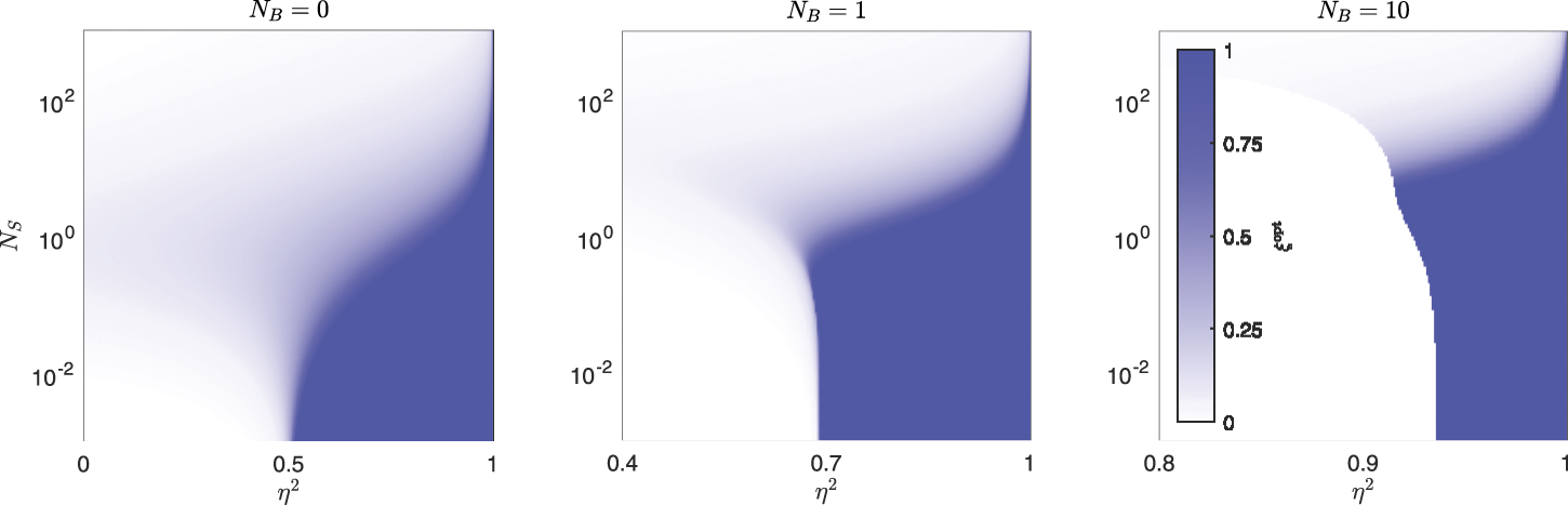