


Abstract
An outlook on the recently proposed quasi-steady quasi-homogeneous (QSQH) theory of the effect of large-scale structures on the near-wall turbulence is provided. The paper focuses on the selection of the filter, which defines the large-scale structures. It gives a brief overview of the QSQH theory, discusses the filter needed to distinguish between large and small scales, and the related issues of the accuracy of the QSQH theory, describes the probe needed for using the QSQH theory, and outlines the procedure of extrapolating the characteristics of near-wall turbulence from medium to high Reynolds numbers.
Export citation and abstract BibTeX RIS

Original content from this work may be used under the terms of the Creative Commons Attribution 3.0 licence. Any further distribution of this work must maintain attribution to the author(s) and the title of the work, journal citation and DOI.
1. Introduction
This paper provides an outlook on the recently proposed quasi-steady quasi-homogeneous (QSQH) theory of the effect of large-scale structures on the near-wall turbulence. The particular question at the focus of the paper is the selection of the filter, which defines the large-scale structures. This is a quickly evolving area of research, and the paper includes a minimalist review of the background and elements of the theory, new results, and a number of conjectures that are yet to be confirmed. To quickly gauge the significance of this new theory the reader already familiar with the landscape of the studies of the effect of large-scale motions on the near-wall turbulence can briefly go forward to figure 2 and formula (4) to see the comparison between the superposition coefficient α(y), introduced in the well-known works of the Melbourne group, and its QSQH theory prediction via the shape of the mean velocity profile U(y). Without the QSQH theory even the existence of any explicit relationship between α(y) and U(y) would be hard to accept. The QSQH theory, however, provides more than just this relationship.
For a wider overview of the current state of research on high-Reynolds-number turbulent near-wall flows the reader is referred to the very comprehensive and quite recent high-quality reviews of the subject, and in particular Marusic et al (2010), Smits et al (2011), Jiménez (2012) and McKeon (2017).
The paper is organized in the following way. Section 2 contains preliminaries including a brief overview of the QSQH theory. Section 3 discusses the filter needed to distinguish large and small scales, and the related issues of the accuracy of the QSQH theory. Section 4 describes the probe needed for using the QSQH theory. The concluding section 5 outlines how the parts described in the preceding sections can be combined for extrapolating the characteristics of near-wall turbulence from medium to high Reynolds numbers.
2. Background
2.1. Conventions
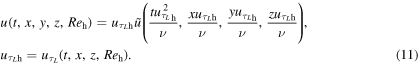
The flow in question is considered to be close to a wall, so that with sufficient accuracy it can be assumed to be statistically homogeneous in wall-parallel directions. A flow in an infinite plane channel satisfies this condition precisely, while boundary layer flows satisfy it only approximately. The flow is also considered to be statistically stationary. The Reynolds number is assumed to be high, so that the flow is turbulent. For simplicity, only one velocity component, denoted u, and directed along the mean flow, is considered. Time is denoted t, the coordinate in the mean flow direction is x. The mean flow direction is also referred to as the longitudinal direction. The wall-normal coordinate is y, and the spanwise coordinate is z.
2.2. Organization of turbulent wall-bounded shear flows
A comprehensive description of a turbulent flow should include both the means for obtaining quantitative answers to various questions and the means for understanding the flow intuitively. An important route to achieving intuitive understanding is to identify relatively simple intrinsic elements of turbulent flow field and then represent the turbulent flow as an ensemble of such elements interacting with each other. Such elements are called organized structures. The most well-known and well understood structure is a near-wall streak, which is an elongated region inside which the instantaneous value of the longitudinal velocity component is below its time-averaged value. In wall-parallel planes near-wall streaks form a partially-regular structure, an example of which is shown in figure 1. Near-wall streaks are present near the wall in all turbulent flows. Streaks have similar dimensions, if measured in wall units. Immediately near the wall the average spanwise distance between the center-lines of streaks, usually referred to as streak spacing, is about 100 wall units, and their average length is about 1000 wall units. As the distance from the wall to the visualization plane increases, the streak spacing also increases, to about 200–300 wall units when the wall distance is 50 and to 400 wall units at the wall distance of about 200, after which it continues to increase (Smith and Metzler 1983). As the distance to the wall increases, near-wall streaks also become less discernible. Hence, the notion of near-wall streaks might be reserved for streaks observed at the distance to the wall below 50–100 wall units. Further away from the wall other structures are observed, namely, hairpin or horseshoe vortices having a continuous range of scales and residing mostly further than 100 wall units from the wall, and large-scales motions and very large-scale motions (usually abbreviated to LSM and VLSM). LSMs can be described as packets of hairpins located more close to the outer edge of the turbulent boundary layer. All LSM dimensions are comparable to the boundary layer thickness, with streamwise LSM dimension being about two to three times larger than the boundary layer thickness. VLSMs are very long narrow regions of low longitudinal velocity residing in the logarithmic and outer part of the flow. VLSM can be observed both in boundary layers and in internal flows. Kim and Adrian (1999) reported that in a pipe flow the length of VLSM could reach 12–14 times the pipe radius. This is about 10 times greater than the largest integral scale in such flows. Various experimental and numerical studies discovered VLSM structures in the logarithmic layer in various flows (Adrian et al 2000, Del Álamo and Jiménez 2003, Tomkins and Adrian 2003, Guala et al 2006, Hutchins and Marusic 2007a, Adrian 2007, Monty et al 2007, Bailey et al 2008, Marusic and Hutchins 2008), including the natural atmospheric surface layer (Marusic and Hutchins 2008). The VLSM structures are often described as packets of hairpin vortices organized coherently along the streamwise direction and meandering in the spanwise direction (Kim and Adrian 1999, Adrian et al 2000, Adrian 2007, Dennis and Nickels 2011a). VLSMs grow in amplitude as the Reynolds number increases (Hutchins and Marusic 2007a). This leads to the formation of a second, so called outer, peak in the energy spectra. Unlike the near-wall streaks, the nature and the quantitative characteristics of large-scale motions appear to be dependent on the particular flow. For example, in turbulent boundary layers it was found (Hutchins and Marusic 2007a, Monty et al 2007) that the length of VLSM structures can exceed 20δ (δ here denotes the thickness of the boundary layer), which is twice as large as reported in other studies. A high-speed stereoscopic PIV experiment (Dennis and Nickels 2011a, 2011b) was used to obtain the velocity information of the entire three-dimensional flow field of a turbulent boundary layer and visualize the VLSM structures by constructing the iso-surfaces of the streamwise velocity fluctuations. The results showed that VLSMs are a concatenation of shorter, several δ in length, substructures, which were not observed earlier due to the limitations of two-dimensional PIV images and poor spatial resolution of previous studies. Since LSM and VLSM were discovered much later than the near-wall streaks, it is natural that so far they are less studied and less understood than near-wall streaks.
Figure 1. Near-wall streaks in a wall-parallel plane. Black areas correspond to regions of low velocity.
Download figure:
Standard image High-resolution imageThere are various explanations of the origin of near-wall streaks, LSMs and VLSMs. Some explanations are based on the idea of filtering properties of the linearized Navier–Stokes operator (Chernyshenko and Baig 2005) and thus do not require consideration of other structures. Other explanations often involve other structures, such as rolls participating in the so called near-wall self-sustaining process (Waleffe 1997). These structures, however, are more difficult to directly observe at high Reynolds numbers. More details about these structures and their relationships can be found in the reviews Smits et al (2011) and McKeon (2017).
For the purposes of this outlook paper it is sufficient to distinguish the small-scale near-wall motions, that is basically near-wall streaks and whatever causes them, and all other, larger structures, which we will collectively call large-scale structures. The QSQH theory, which will be reviewed next, in the first approximation can be considered as the theory describing how these large-scale structures affect the small-scale near-wall structures.
2.3. QSQH theory
The near-wall region where near-wall streaks reside is traditionally considered as scaled appropriately in the wall units, that is units based on the time-averaged wall friction  , kinematic viscosity ν and density ρ. Such scaling is based on dimensional and asymptotic arguments for the case of the Reynolds number tending to infinity. The classical view, which we will call the classical universality hypothesis, is that as
  while y+ = const, the flow velocity tends to a function independent of the Reynolds number:

where the friction velocity  and the superscript + marks quantities non-dimensionalized with the wall units. Note that the above representation, while convenient and widely used, requires a clarification. If understood literally, (1) implies a sequence of experiments conducted at the same conditions but with a sequence of
  n = 1, ..., which is increased from experiment to experiment tending to infinity, while the corresponding u = un is converging to its limit. In fact, since turbulent flows are chaotic and highly sensitive to perturbations, the instantaneous velocity fields un are quite different, and the sequence un does not converge. Instead, the convergence is understood here in a probabilistic sense as convergence of all possible statistical characteristics of un to the
  -independent statistical characteristics of a random function
  . This remark applies also to other similar situations in the present paper.
The classical universality hypothesis (1) was widely accepted for a long time, but eventually it became clear that it is unlikely to be correct, because even close to the wall the flow is affected by the large-scale structures, and because the magnitude of the influence of large-scale structures on near-wall structures, measured in wall units, depends on  even when
  . The effect of large-scale motions on near-wall turbulence was clearly demonstrated in the widely-known series of studies (Hutchins and Marusic 2007b, Mathis et al 2011, Ganapathisubramani et al 2012) and (Mathis et al 2013).
These works rely on a representation of the velocity field as a sum of a large-scale and a small-scale components:

where the large-scale component is usually obtained from a time-dependent signal by a low-pass filter, and two probes measure simultaneously the velocity in the flow, with the near-wall probe placed closer to the wall than the outer probe. This series of studies provide a strong experimental and numerical evidence that there exist such Reynolds number-independent functions 
 and
and  that at high
Here primes denote fluctuations, the subscript L denotes low-pass-filtered, that is large-scale, quantities, and  is the coordinate of the outer probe. Note that (2) is compatible with (1) only if the dependence of
  on
on  becomes negligible as
  . However, in the last two decades an overwhelming evidence to the contrary was accumulated. In fact, the amplitude of fluctuations of
  grows as
  increases (see again the reviews cited above). It is clear that the classical universality hypothesis has to be revised. The QSQH theory is the first step towards such a revision.
Unlike (1), (2) was obtained empirically, without any theoretical justification. It does, however, provide a hint for the possible improvement of (1). While the right-hand side of (2) is  -dependent, this dependence enters the formula only via a single large-scale-filtered quantity. It is natural to expect that large-scale-filtered quantities vary slowly in time, which makes them similar to time-averaged quantities. This idea of quasi-steadiness of large-scale motions as far as near-wall turbulence is concerned is behind the main hypothesis of the QSQH theory, which amounts to replacing the friction velocity uτ based on the time-averaged skin friction with its large-scale analog
  Naturally,
  depends on time and the coordinates at the wall, but not on the wall-normal coordinate. Then, instead of (1), QSQH hypothesis postulates that at high
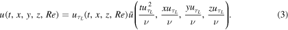
Here,  is a non-dimensional velocity, similar to u+ in the classical universality hypothesis (1). The difference is that the velocity scale, uτ, used in the classical universality hypothesis, is a constant independent of the fluctuations of the large-scale structures, while in the QSQH hypothesis (3) the velocity scale
  fluctuates in unison with the large scales motions. Importantly, the same is true for the time and length scales,
  and
and  respectively, as indicated by the arguments of
  in (3). This defines the nature of the effect of large-scale fluctuations on the near-wall motion. In the absence of large-scale fluctuations one would have
  and (3) would coincide with (1), giving
  When the large scales fluctuate,
  is multiplied by a fluctuating quantity
  . Using the standard terminology, this can be described as an amplitude modulation of
  by
by  Amplitude modulation is not the only mode, or mechanism, by which, according to (3), the large-scale motions affect the near-wall motion. Fluctuations of the large scales lead to the fluctuation of the time scale too, (so that we have
  with
with  also depending on t via
  ). This type of influence of one characteristic on another is usually described as frequency modulation. Similarly, the variation of the length scale
  in (3) can be described as length scale modulation. Notably, while the QSQH hypothesis (3) involves amplitude, frequency, and length scale modulation, it does not involve another well-known type of relationship between two entities, that is superposition, which would lead to an extra additive term in (3) depending only on the large-scale motions. We will explain later the seeming contradiction with the empirically verified relation (2), which contains a superposition term
  . It might be appropriate here to mention that frequency modulation in the context of scale interaction in near-wall turbulence was investigated in Ganapathisubramani et al (2012), and that wall-normal scale modulation was implied by the explanation of the reversal of the correlation between large-scale motion and the intensity of the wall-normal fluctuations, proposed in Jiménez (2012).
In the QSQH theory the function  introduced by (3) is universal in the sense that all its statistical characteristics are independent of
  and of the other large-scale factors such as the geometry of the entire flow and the pressure gradient. This is similar to the universality of the statistical characteristics of u+ in (1) and of
  in (2). There is, however, an important difference. The statistical properties of large-scale fluctuations and, hence, of
  do depend on
  and the other factors. Because of this, the universality of the statistical properties of
  implies its statistical independence of
  as otherwise the function
  would depend on
  On the other hand, one has to distinguish a function from its value at a given value of its arguments. Let us, for the sake of illustration only, assume for a moment that
  and that A is a random quantity, while
  is another random quantity. Then, the statistical independence of
  and the function
  is the same as the statistical independence of
  and A. Consider now the value of
  Clearly, even though A and
  are statistically independent,
  and
and  are statistically dependent. Thus, in (3),
  and
and  are statistically dependent, which makes (3) rather nontrivial, but
  and the function
  are statistically independent, which allows to efficiently use the tools of mathematical statistics for deriving from (3) relationships relating various quantities of interest. For details of such mathematical derivations the reader is referred to Zhang and Chernyshenko (2016).
To use the QSQH theory for obtaining quantitative results one needs to fully define the large-scale filter. The choice of the filter determines how well the QSQH hypothesis (that is (3), statistical independence of  and
and  , and the
  -independence of
  ) is satisfied in the real turbulent flow. The properties of this filter also determine the results of analytic derivations and qualitative analysis on the basis of the QSQH theory, and how easy the analytic derivations and qualitative analysis will be. In Zhang and Chernyshenko (2016) these two questions were separated. The properties of the filter sufficient for analytic derivations and qualitative analysis were specified as an essential component of the QSQH theory, without specifying the filter exactly. Abstracting from the unnecessary detail proved to be a powerful tool for developing the theory. However, the responsibility of defining the filter exactly was left with the end user, who was expected to select the filter with the best possible performance both in terms of the QSQH hypothesis and postulated filter properties, and with the view of the specific goals of the end user. In Zhang and Chernyshenko (2016) multi-objective optimization was used to narrow the choice to a Pareto front, guided by the particular interest in certain forms of turbulent drag reduction. The point on the Pareto front was selected then using an 'educated guess', thus defining a particular filter for quantitative comparisons, but no further analysis was presented concerning filter selection. This will be the subject of section 3 of the present paper.
Prior to pointing out a number of important issues concerning the QSQH theory and its interpretation, it makes sense to demonstrate both its potential and its limitations, by providing some comparisons. The superposition coefficient α(y, yo) in (2) was introduced by Mathis et al (2011) as
where  is the large-scale-filtered velocity fluctuation, and
  denotes averaging.
In Chernyshenko et al (2012) on the basis of the QSQH theory it was predicted that α(y, yo) and the mean velocity profile U(y) are related, namely

Another example is the correlation between the large-scale friction velocity fluctuation  and the square of the small-scale velocity fluctuation
  , which can be characterized by coefficient γ1 defined as

The QSQH theory predicts (Zhang and Chernyshenko 2016) that
where  is the root mean square of the velocity fluctuation. Here and everywhere in this text the velocity is non-dimensionalized with the average of the dimensional version of
  the same as in Zhang and Chernyshenko (2016). Note that (4) and (6) are nontrivial and would be difficult to obtain empirically. Many more such relationships are derived in Zhang and Chernyshenko (2016). Note also that even within the QSQH theory (4) and (6) are approximate: they were obtained by expanding in powers of
  the exact relationships given by the QSQH theory. The comparisons are shown in figure 2. The agreement for α is very good, while γ1 discrepancy is of the order of 10%, which is also the degree of discrepancy reported in Zhang and Chernyshenko (2016) for other comparisons. While, obviously, at least a part of this 10% can be due to the truncation of the Taylor expansion, the QSQH theory itself is approximate only, as we will discuss in section 3. However, the nontrivial nature of these results and the degree of agreement do show that the QSQH theory captures a major part of the issue of scale interaction in near-wall turbulence and, therefore, deserves further attention.

Figure 2. Coefficients α and γ1 for  The curves are the QSQH prediction (4) and (6), the symbols are derived from the direct numerical simulation of the plane channel flow at
  (Sillero and Jiménez 2016). No cut-off in time was used, and the spatial cut-off lengths were Lx = 4200 and Lz = 628.
Download figure:
Standard image High-resolution imageThree important issues should be highlighted without delving deep into the underlying mathematics. First, the QSQH theory partially confirms the empirical formula (2) by demonstrating (Chernyshenko et al 2012) that (2) is the main term of the Taylor expansion of (3) in powers of  However, the QSQH theory gives a different physical interpretation of the term containing α in (2). When this term was introduced, it was interpreted physically as a superposition of large-scale structures on the small-scale motion near the wall. The QSQH hypothesis (3), however, does not involve the superposition mechanism, as we have already pointed out. From the details of the derivation of (4), for which the reader is referred to the original papers, it follows that the term with U(y) in the expression (4) for α appears due to the amplitude modulation mechanism, and the term with
  appears due to the wall-normal-scale modulation. Hence, in physical interpretations of the various effects of large-scale motions on the near-wall turbulence this combination of amplitude and scale modulation should be used instead of the notion of superposition. The term with α in (2), usually referred to as the superposition term, is in fact a linear approximation of the combined effect of amplitude and frequency modulation.
The second issue is the relative significance of the amplitude and scale modulation mechanisms. Taking into account the scale-modulation mechanism is more difficult than taking into account the amplitude-modulation mechanism, since it requires the data to be collected and analyzed at a point in space moving in response to variation of  For example, to keep the value of the third argument
  of
of  constant and equal to a fixed value
  , the observation point y should vary in time and space as
  . Hence it might be tempting to ignore scale modulation. However, the specific results indicate that quantitatively the scale modulation is at least as important as the amplitude modulation. For example, in (4) the amplitude modulation contribution to α is proportional to U(y) and the scale modulation contribution is proportional to
  , which means that their ratio tends to unity as the wall is approached. For
  the scale-modulation mechanism is responsible for the section with negative slope of γ1(y), where this mechanism overcomes the contribution of the amplitude modulation (see figure 11 and the related discussion in Zhang and Chernyshenko (2016)). Therefore, any considerations based on the QSQH theory should always take into account the scale modulation element of the theory.
The third issue is related to the importance of nonlinearity of the QSQH theory with respect to the magnitude of the large-scale fluctuation  . At the moderate values of
  achievable in direct numerical simulations this magnitude is quite small. For the large-scale filter used in Zhang and Chernyshenko (2016)
  (in wall units). However, in the context of the QSQH theory it often turns out to be multiplied by a large quantity. For example, in (6)
  is multiplied by
  . Approximated using the logarithmic law
  with typical constants κ = 0.4, B = 5 this factor is about 360 at y+ = 100, and 0.004 4 · 360 ≈ 1.6, which is not small. For this reason one should always distinguish the full QSQH theory and its approximations based on the assumption that
  This is particularly true when higher
  or variations with
  or particularly large values of
  are involved.
2.4. Subjective nature of the universal velocity field in the QSQH theory
The main relationship (3) of the QSQH theory allows to calculate the statistical properties of the universal velocity  provided that the large-scale filter is defined. An important question is whether there is only one suitable filter. If yes, then the universal velocity is an objective element of the physical world. If there are many equally suitable filters then the definition of
  involves a subjective selection of one of the filters by the researcher. If, as it is the case, the theory is approximate, and in practice the filters satisfy the required properties only approximately, the question of the uniqueness of the best filter becomes particularly important. Moreover, if there are many equally suitable filters then different suitable filters should lead to the same predictions about the physical reality, and an explanation of how this can be possible is required.
While these questions are yet far from being fully answered, certain observations suggest a negative answer. In other words, it is likely that there is no unique best, or 'correct', filter. In this section these observations are described and a conceptual explanation of the possibility to obtain results independent of the subjective choice of a particular filter among the suitable filters is given. This explanation will also cover the issue of the reason how the QSQH theory can give reasonable results (exemplified by figure 2) in spite of the continuity of the turbulence spectrum and the energy contained in the intermediate scales not being small, that is the actual situation being rather different from the situation with a spectral gap.
We will consider the example of using the QSQH theory for the analysis of the dependence of the root mean square fluctuation velocity on  For simplicity, we will assume that
  which will allow to use equation (21) from Zhang and Chernyshenko (2016) rewritten as

in which we replaced the universal mean velocity  with the mean velocity profile U, since they are very close when
  . In (7)
  is the the value at η = y of the root mean square of the fluctuations of
  (with the mean taken over
  and
and  while η is held constant). Therefore, if the filter is known one can calculate both
  and
and  and verify (7). We performed such a comparison with satisfactory results. For the purposes of this paper, however, it is particularly instructive to consider what happens when one changes the choice of the filter and the value of
  . If the filter is the same and
  changes then both
  and
and  change but
  should remain the same. It can, hence, be eliminated by subtracting two versions of (7) at different
  , obtaining

(Close to the wall, where QSQH theory applies, the mean profile also does not change when  changes.) One can further take a logarithm and differentiate with respect to y, thus eliminating
  entirely and arriving at a nontrivial equality, the validity of which was confirmed by comparisons in figure 12 of Zhang and Chernyshenko (2016). If (8) applies for different filters then
  should be independent of the choice of the filter even though
  does depend on it. The comparisons in Zhang and Chernyshenko (2016) and further comparisons we made so far confirm this remarkable property. It is, indeed, in agreement with the current understanding of the evolution of the spectra of turbulent flow as
  increases.
Figure 3 illustrates this. It shows schematically the spectra for two different  . The vertical line denotes the cut-off of the filter. The area beneath the curves and to the right of the cut-off represents the large-scale energy
  . There is no spectral gap, so that the change of the cut-off length changes
  . However, as far as the cut-off remains within the part of the spectra that does not change with
  , the variation of
  with
with  will be independent of the filter choice. In practice,
  can only be obtained from experimental or numerical data at a particular
  , and the QSQH theory then can be used for predicting the flow properties at higher
  .
.

Figure 3. Schematic representation of the energy spectral density Φ as a function of the length scale l for two values of 
Download figure:
Standard image High-resolution image3. Filter
3.1. Filter properties
The QSQH theory postulates that the large-scale filter has certain five properties (Zhang and Chernyshenko 2016). If such a filter is impossible, the entire theory would be self-contradictory, but two examples of such filters were given in sections IIB and VI of Zhang and Chernyshenko (2016), confirming the self-consistency of the theory. Four of these properties, namely, linearity, invariance of averages (the large-scale filter applied to an averaged quantity does not change it), the projection property (the large-scale filter does not change an already large-scale-filtered variable), and commuting with averaging (the average of large-scale-filtered variable equals the average of the unfiltered variable) are easier to understand and are satisfied, for example, by a Fourier cut-off filter. The fifth property, however, can be satisfied only by rather special filters. The fifth property is the scale-separation property, formulated in Zhang and Chernyshenko (2016) in the following way: 'applying the large-scale filter to any function of t, x, y, z, and other arguments that are large-scale-filtered variables is equivalent to averaging over the homogeneous directions and/or time t, x and z with the other arguments held constant'. In the mathematical derivations of (Zhang and Chernyshenko 2016) this property is used formally: where convenient, the large-scale-filtered function is replaced with its average exactly as stated. It is not known whether a filter exactly satisfying all the five properties and at the same time useful for the study of the effect of large-scale motion on the near-wall turbulence actually exists. In practice, the end user of the theory needs to select a filter satisfying this property at least approximately, and for this an intuitive understanding of this property is desirable. This can be helped by two examples.
The first example is an an infinite time averaging used as a large-scale filter. In this case verifying the five properties is trivial. However, in this case the large-scale quantities do not fluctuate at all,  , and the QSQH hypothesis reduces to the classical universality hypothesis, which is known to be inaccurate and which the QSQH theory is supposed to improve. A finite-time averaging over a sliding window, the size of which is much smaller than the characteristic time scale of the large-scale motions can be better from the viewpoint of satisfying the QSQH hypothesis, but it does not exactly satisfy, for example, the projection property.
The second example is a Fourier cut-off filter. The cut-offs could be selected in such a way that the fifth property would be satisfied if the actual velocity distribution had an infinitely large (say, tending to infinity as  ) spectral gap between the large and small scales. Note also that the main QSQH hypothesis (3) also implies such a gap, in the sense that for it to be exactly accurate, the large scales should be much larger than the small scales, and there should be no intermediate scales at all. It is equivalent also to averaging over a sliding window the size of which is much greater than the largest time-scale of the small-scale motions and at the same time much smaller than the smallest time scale of the large-scale motions. Instead of time scales, spatial scales would also be acceptable here. These requirements on the relation of scales might be considered as one of the most intuitively obvious ways of satisfying the fifth property of the ideal filter. To satisfy these requirements, the large-scales should be much larger than the small scales. The ratio of largest scales to smallest scales in turbulent flows increases as
  increases, which means that the QSQH theory can be expected to give better results for higher
  . However, for actual turbulence, a Fourier cut-off filter also cannot exactly satisfy all the requirements, because the turbulence spectrum is continuous, that is the largest of the small scales coincide with the smallest of the large scales. Therefore, it seems highly likely that a filter exactly satisfying all these requirements and ensuring also that the QSQH hypothesis is exactly accurate does not exist.
Hence, in specific applications selecting the filter has to involve a compromise, which implies a multi-objective optimization. It is also a constrained optimization, since not every filter imaginable can be applied to every case in question. For example, if the only data that is available is a single-point time series then a spanwise Fourier cut-off filter cannot be applied, while the time Fourier cut-off filter can.
3.2. Filter selection
The general idea of finding a suitable filter following the example given in Zhang and Chernyshenko (2016) consists in the following. First, the data set to which the filter is to be applied is considered, and a set of filters that can be applied to this data set and satisfy at least approximately the required five properties is identified. It can be expected that this set will contain more than one filter, for example, it can be a set of Fourier cut-off filters with a range of the cut-off values. Second, a set of quantifiable parameters πi, i = 1, ..., N with not too large N characterizing the accuracy of the QSQH theory and other desirable properties of the particular filter is selected. Then calculations of π1, ..., πN for various filters are performed until the Pareto front, that is a surface in the π1, ..., πN space separating the points (π1, ..., πN) that can be obtained with at least one applicable filter from the points that cannot be obtained with any applicable filter is identified. The Pareto front thus represents the set of optimal filters, and then further choice of the specific filter has to be done in view of the shape of the Pareto front and some additional considerations.
For example, in Zhang and Chernyshenko (2016) this idea was applied to the data on a plane channel flow obtained in direct numerical simulations, so that a Fourier cut-off filters with cut-offs in time and two wall-parallel directions were applicable. Two parameters characterizing the desirable properties were selected: the correlation coefficient  between the large-scale fluctuations very close to the wall and the large-scale fluctuations at
  and the correlation coefficient
  between small-scale fluctuations at the same locations. From (4) it follows that rLL ≈ 1, according to the QSQH theory for
  case, so it is desirable to select the filter with rLL close to 1. On the other hand, given the declared in (Zhang and Chernyshenko 2016) motivation of applying the theory to predicting the effect of the Reynolds number on the degree of drag reduction by technologies affecting the near-wall flow, it is of interest to have rSS small. Selecting a particular combination of the cut-offs in time and two wall-parallel directions fully specifies the filter, and allows to calculate rLL and rSS, which is then plotted as a point in the rLL–rSS plane. This is repeated for a very large number of the cut-off combinations, thus obtaining a cluster of points. It was observed that these points fill in an area adjacent to the top left corner. Then all these points except those that were judged to be at the border of this area were removed, and the remaining points were considered as the approximation of the Pareto front. Any combination of rLL and rSS above and to the left of this Pareto front could be obtained with at least one Fourier cut-off filter, while no filter could give the combination of rLL and rSS to the right and below the Pareto front. Several Pareto fronts obtained with different filters and at different
  different from Zhang and Chernyshenko (2016) are shown in figure 4. One can see that each of the Pareto fronts describe the trade-off between rLL and rSS, since for each point on the Pareto front improving rLL (that is moving to the right) can be achieved only at the expense of deterioration of (that is a rise in) rSS. It does not make sense to select a filter corresponding to the inside of the feasible area above and to the left from the Pareto front, since a filter with better both rLL and rSS exists. However, the choice between the filters on the Pareto front has to be made on the basis of additional considerations.

Figure 4. Pareto fronts, experimental data: - - - - , (Rodríguez-López et al 2016), –·–
 (Baars et al 2015), direct numerical simulation data (Lozano-Durán and Jiménez 2014): ◯
 , □
, □ ,
,  .
.
Download figure:
Standard image High-resolution imageIn the present study we use the same set of the filter performance characteristics, rLL and rSS, to investigate the relative quality of filters of a different type and at different  Two of the Pareto fronts in figure 4 were obtained on the basis of experimental data and three Pareto fronts were obtained from direct numerical simulation. The experimental data consist of only time series at two points at different distances from the wall. Accordingly, a Fourier filter with the cut-off only in time could be used. The direct numerical simulation data are more complete. The Pareto fronts based on numerical data, shown in figure 4, were obtained with Fourier filter with cut-offs in two wall-parallel directions but not in time. As it could be expected, as
  increases the Pareto fronts shift towards the bottom-right corner, thus indicating that the overall performance of the QSQH theory improves. However, a much larger difference between the Pareto fronts is due to the change in the nature of the filters: having two spatial cut-offs instead of one temporal cut-off gives much better results.
It is interesting to note that for certain range of the values of the cut-offs rSS is negative. We attribute this behavior to the time lag between large and small scales, but more research is needed before a definite conclusion can be made.
Experimental data usually contain only the time series, but, as we can see from figure 4, this is not enough to properly detect the large-scale motion. Assuming that the Taylor hypothesis being approximately valid for large-scale motions, cut-offs in time and in the longitudinal directions should be equivalent. Hence, it is the loss of the cut-off in the spanwise direction that leads to a rather substantial deterioration of the quality of the filter. The importance of the spanwise direction for properly detecting large-scale motion was also noticed in Kerherv et al (2017), where a complicated experimental and data-processing technique was proposed. Another possible solution to this problem is described in the following section.
4. The probe
We propose to use a probe consisting a spanwise rake of sensors as shown in figure 5. For applications of the QSQH theory the probe should be as close to the wall as possible. (Ideally, it should measure the wall friction.) Since this might be difficult, sensors located at the distance yo+ up to about 100 wall units from the wall can be used, since the large-scale motions are reasonably well correlated in wall-normal direction up to this distance (Zhang and Chernyshenko 2016). The probe will be used to measure approximately the large-scale-filtered velocity, and the large-scale friction will then be obtained with the help of the QSQH theory. The approximation  for the actual
  is obtained in the following way. First, a Fourier cut-off filter in x direction, but not z direction, and with the same cut-off length
  as the large-scale filter, is applied to
  giving a partially filtered field
  Then the approximation for the large-scale filtered field is obtained from the formula

where  is the spanwise displacement of the kth sensor within the rake, and n is the number of the sensors. The weights wk and the sensor displacements
  should be optimized to minimize the difference between
  and the actual uL.

Figure 5. The probe consisting of a rake of velocity sensors.
Download figure:
Standard image High-resolution imageThese optimal probe parameters depend on the basis set of data and the particular filter used to determine the statistics of the universal velocity field  We will now describe the probe optimization we performed for the plane channel flow database for
  (Sillero and Jiménez 2016) taken as the basis set, and the large-scale filter taken as a spatial Fourier cut-off filter with the cut-off lengths
  and
and  selected in Zhang and Chernyshenko (2016). In that paper the cut-offs were selected from the Pareto front at
  Therefore, using the same cut-offs for higher
  should keep the filter in the area of the spectrum not strongly affected by increase in
  as suggested in section 3. At the same time this misses the opportunity to improve the accuracy of the QSQH predictions by adjusting the cut-offs to the higher-
 database, which can be done in the future. In Zhang and Chernyshenko (2016) the filter also included a cut-off in time, but here we observed that, thanks to a much larger size of the computational box for
  the time cut-off can be dropped. In experiments using a cut-off in x will not be possible, and, hence, using the cut-off in x as a proxy for cut-off in time is the best option in optimizing the probe. However, ideally, the cut-off values should be selected to correspond to
  of the database to be used for optimization.
The optimal probe was determined in the following way. One randomly selected time frame from the database was used. The grid layer at  provided a slice of the velocity in the form
  where
where  and
and  are the grid line coordinates. Applying to this slice the Fourier cut-off filter described above gave the corresponding large-scale component
  The number of sensors n = 9 was assumed after consultations concerning a possible future experimental implementation. The optimal weights wk and sensor displacements
  were found by minimizing over wk and
  the L2 norm
of the difference between uL and  , with
  defined by (9). Optimization over wk is a simple quadratic optimization. In the first instance the sensors were assumed to be evenly spaced,
  and the optimization over
  was done by a line search. In the second approach the sensor displacements were optimized using the genetic optimization algorithm included in MATLAB. The sensor displacements were assumed to be symmetric with respect to the center sensor, but the weights were optimized for all nine sensors, and the symmetry of the obtained weights served as an additional test for the consistency of the optimization procedure. On a visual inspection the large-scale fields
  and
and  were close. The relative error
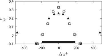
  was about 0.07 for the genetically optimized probe and about 0.08 for a constant spacing probe. The optimized probe was then used to obtain an approximation for the large-scale field from a different time snapshot in the database, and this gave the relative errors of about 0.08 and 0.09 respectively. For uniformly-spaced probes the sensor spacing was found to be Δz+ = 64.13. The weights and the relative positions of the sensors of the uniformly-spaced optimized probe and of the genetically optimized probe are given in table 1, and illustrated in figure 6. We give the results with 4 digits, which are valid for a particular time frame from the database, but observing the variation of the result from one time frame to another we believe that only two digits here are significant.
Figure 6. Weights:  uniform
  □ uniform
  genetically optimized
  The horizontal bar shows the cut-off length.
Download figure:
Standard image High-resolution image
Table 1.
Positions and weights of sensors of the optimized probes, approximating the Fourier cut-off filter with the cut-off lengths  and
and  Only two digits are expected to be significant, and the relative approximation error is believed to be about 0.08 for the non-uniformly spaced sensors and 0.09 for the uniformly spaced sensors.
| Uniform spacing | Non-uniform spacing | |||
|---|---|---|---|---|
| k | 
|
wk | 
|
wk |
| 5 | 0 | 0.330 6 | 0 | 0.256 4 |
| 4 and 6 | ±64.13 | 0.278 3 | ±51.3 | 0.248 2 |
| 3 and 7 | ±128.26 | 0.136 9 | ±111.6 | 0.197 9 |
| 2 and 8 | ±192.39 | 0.005 0 | ±260.8 | −0.099 9 |
| 1 and 9 | ±256.52 | −0.093 2 | ±478.8 | 0.032 2 |
The same procedure was repeated for the database for  , but for uniformly-spaced probes only. Importantly, it turns out that the Reynolds number has little effect on the optimal probe. The main effect of the genetic optimization amounts to moving the sensor that has almost zero weight in the uniformly-spaced probe to a new position. Calculations with different cut-off lengths within a reasonable range were also done, and did not lead to large variations of the optimal probe.
5. Outlook and conclusion
One of the prospective uses of the QSQH theory is an extrapolation of near-wall turbulence characteristics to larger values of the Reynolds number, for which full numerical calculations and near-wall experimental measurements are more difficult. Such an application requires several elements.
First, a comprehensive turbulent flow database at a moderate  should be selected, which contains the velocity field
  . Databases of high-Reynolds-number direct numerical simulations of fluid flows might be the most appropriate type of databases for this purpose.
Second, the large-scale filter should be selected using the Pareto front technique and the additional considerations as described in section 3. If accuracy of about 10% is considered as acceptable, the Fourier cut-off filter with cut-offs in wall-parallel directions  and
and  can be used. The filter will complement the velocity field
  with the corresponding large-scale field
  . We will call the pair
  and
and  the base data set.
Third, using the data from the base data set, the large-scale probe rake parameters should be determined by the procedure described in section 4. If accuracy of about 10% is considered as acceptable, the rake with 9 sensors and the parameters obtained in section 4 can be used. More sensors, higher  base data set, and revised (increased) cut-off lengths are required for better accuracy.
Fourth, measurements of  are made at the high
  using the probe. This is easier than measuring
  because
  can be determined from measurements further away from the wall using the QSQH theory and because, being large-scale, it requires less spatial and temporal resolution.
Finally, the collected data are used to predict the statistical characteristics of  . This is done in the following way. The QSQH hypothesis (3) is rewritten as

This uses new variables
The base data set provides, via (10), the full statistical description of  . Then, (3) is again rewritten, this time as
This gives the full statistical characteristics of  . A preliminary testing of a part of this procedure using only numerical databases is described in Chernyshenko et al (2017). The next step is to test the full procedure in an experiment.
So far the analysis was restricted to the longitudinal velocity only. Extending it to spanwise and wall-normal velocities would be the most natural continuation of the development of the QSQH theory.
The large-scale motions depend not only on the Reynolds number but also on the pressure gradient and flow geometry while the statistical properties of the universal velocity  , introduced in the QSQH theory, are independent of them. Therefore, the QSQH extrapolation approach can be used to predict the effect of pressure gradient and flow geometry on the properties of near-wall turbulence. This can be tested by numerical calculations or a physical experiment.
An even more ambitious aim is developing full asymptotic representations of the flow statistics in the entire flow domain for canonical flows, such as the plane channel, pipe, and flat plate boundary layer. Such an asymptotic representation might be expected to have a two-layered structure, with different representations in each layer, and with an overlapping region of validity, which is the asymptotic structure commonly encountered in fluid dynamics, as exemplified by a boundary layer and an inviscid outer flow. The QSQH theory would provide an approximate description of the near-wall layer. The most efficient way of providing a full statistical description is a sufficiently large database of instantaneous flow parameters, ideally a database of the universal velocity arising in the QSQH theory. A similar database of the Reynolds number universal velocity would need to be created for the flow in the outer part. This, of course, requires first developing the asymptotic theory for the outer part of the flow, which is a goal actively pursued by the research community, but which might yet be out of reach.
Acknowledgments
This work was supported in part by the International Project Research, 'Fluid Dynamics of Near-Wall Turbulence', promoted in 2016 by the Research Institute for Mathematical Sciences (RIMS), a Joint Usage/Research Center located in Kyoto University.
This work originated from studies done under EPSRC UK grant EP/G061556/1.