

Abstract
This paper theoretically, numerically and experimentally investigates the autofocusing properties of chirp beams with arbitrary power law dependence on the radius. It was demonstrated that the use of superlinear chirp (radial phase dependence with a power greater than 2) provides faster and more abrupt focusing than circular Airy beams. The use of two- and three-parametric chirp beams allows the effective control of the autofocusing properties of circular beams in various applications in optics and photonics.
Export citation and abstract BibTeX RIS
1. Introduction
Recently, researchers have focused on different beams with autofocusing properties [1–8], including circular Airy beams, Pearcey beams, and hyper-geometric beams. The abrupt autofocusing properties inherent in such beams are required for optical manipulation [9, 10], and are useful for multiphoton polymerisation [11], nonlinear effects [12] and for polarisation transformation [13, 14].
The lens is a classic focusing element which has a quadratic phase dependence on the radius. The diffractive version of the refractive (classic) parabolic lens looks like a zone plate with circular lines condensing to the edge of the optical element as a linear chirp (the frequency of rings increases linearly with the increasing radius). Consequently, circular Airy beams, which have an asymptotic phase dependence proportional to  were identified as a sublinear chirp [3], and beams with a dependence on
  when 1 < q < 2 have been investigated.
In the present paper, we consider laser beams which have a radial phase dependence proportional to  when q takes any positive real value (q > 0), including q > 2, i.e. superlinear chirp. Optical elements with such phase dependence can be called generalised lenses [15] or fractional axicons [16]. This paper theoretically, numerically and experimentally investigates circular superlinear chirp beams (CSCBs), demonstrating that they provide faster and more abrupt focusing than circular Airy beams. Two- and three-parametric chirp beams with controlled autofocusing properties have the potential for a wide range of applications in optics and photonics.
2. Theoretical analysis
In contrast to previously considered abruptly autofocusing beams based on Airy functions [1–3], equation (1) provides the superlinear chirp dependence of the Airy function on the radius:
where  is the Airy function [17], n is the degree of nonlinearity of the radius,
  is the circle function with unit amplitude, R is the radius of the input field,
  is the radial displacement parameter and w is the normalising parameter.
A rigorous theoretical analysis of the beam properties having the input amplitude (1) is rather complicated. Nonetheless, for qualitative evaluations, it can be used for the approximation of expression (1) by another function, also having oscillations with a varying frequency and amplitude:
where the values q and p are not necessarily integers. In particular, for a function, assigned by equation (1), 
Equation (2) is principally close to the approximation considered in [3]. However, the authors considered the case for  which corresponds to the input distribution oscillation more slowly than the linear chirp. A more general situation is considered in this work, such as q > 0, which involves the oscillation of input distribution faster than linear chirp. In addition, primary functions without radial displacement and then with the presence of displacement are investigated.
2.1. Two-parametric chirp-beams
Without losing generality, p was set to 0 and  was taken into account. First, regarding the case without radial displacement, i.e. when r0 = 0, it can be proved that the contribution of the first exponent to the formation of focal distribution is small, so it is assumed that the input field has the following form:

where q is the chirp order,  is the wave number, λ is the wavelength of the illuminative radiation and
  is the dimensionless parameter related to the numeral aperture (NA) of the focusing element, defined by equation (3), as follows [15]:

Beams, formed with the help of the focusing element defined by equation (3), are known as two-parameter (q and α0) chirp beams. The fact that an optical element, having a complex transmission function described by equation (3), is focusing is obvious, particularly when q = 2 and equation (3) corresponds to a parabolic lens. The diffraction version of a parabolic lens has a line structure, which can be called the linear chirp. The Airy function in equation (1), when n = 1, corresponds to q = 3/2, i.e. a sublinear chirp [3]. The value of q > 2 corresponds to the superlinear chirp.
To understand the qualitative relationship, beam propagation in free space was considered using the Fresnel transformation:
Taking into account the radial symmetry of the optical field described by equation (3), we may set θ = 0:
The angle integral in equation (6) can be calculated analytically, and it is equal to the Bessel function. However, the resulting radial integral may be calculated analytically in very rare cases, even for the field on the optical axis, but the use of approximate analytical methods in the presence of the Bessel function in the integral leads to an increase in the error. Therefore, the integral by polar angle based on the stationary phase method [18] was considered, taking into account two stationary points (φ = 0 and φ = π):
If the curly bracket in equation (7) is  it corresponds to the asymptotic representation of the exact value
Using equation (5) and geometric-optical considerations ensures that the second term is the main one in the curly brackets of equation (7), which corresponds to the stationary point at 0 degrees. The calculation can be performed using the following formula:
Note that equation (8) is not applicable near the axis.
Next, considering the integral in equation (8), the stationary phase method can be applied. For the function in equation (3), the stationary point can be obtained from the equation:

There is one (non-zero) stationary point [15] for q < 2 (sublinear chirp) at any ρ. The situation changes significantly for q > 2, when two stationary points exist or are absent. The merging of two stationary points means the availability of not just the maximum, but caustics. The caustics exist when function values and derivatives are equal at stationary points. Then, in addition to equation (9), the following equation is fulfilled:

Equation (10) is always solvable, and the value of the stationary point  when derivatives are equal can be calculated:

Substituting the value from equation (11) in equation (9), after algebraic manipulations, the necessary condition for double root that describes the focal line shape (the caustic) is obtained:
As q > 2, caustic lines in equation (12) have a shape resembling a hyperbola and theoretically do not cross the optical axis. In particular:
As follows from equation (12), when the value of q increases, the focal lines approach the optical axis more slowly. This is quite understandable, as for large q, a central part of the input field is close to the plane wave. At the infinity limit,  i.e. the distribution looks like a ring with a constant radius, which shrinks into a point suddenly at some distance. This occurs because there is a caustic on the optical axis, except the caustic defined by equation (12). The fact that the axisymmetric element has two types of caustics, namely, the axial caustic and the caustic of rotation, was proved in [19].
To consider the case on the optical axis, ρ = 0 can be directly substituted into equation (6):
Using the classic stationary phase method [18] to equation (13) for the function from equation (3), the intensity on the optical axis [15, 16] is as follows:
Equation (14) is correct for any q > 0 outside the shadow area.
For 0 < q < 2, the intensity on the axis increases with the increasing distance (in particular, for q = 3/2  ) until the moment corresponding to the arrival of rays from the edge (or border of the entrance pupil) of the optical element [16]. In contrast, for q > 2, at first, a shadow segment is on the axis, then there is sharp jump of intensity [15], which decreases with increasing distance (in particular, for q = 3
  ).
).
It is of note that there are two caustics, one defined by equation (12), and the other is on the optical axis, whose intensity dependence on distance is described by equation (14). Thus, for q > 2, the focus is just formed by axial caustics and its position is close to the position of intensity's sharp jump after a shadow. More accurate calculations using the modified stationary phase method [15] lead to the following expression for the distance of maximal intensity on the optical axis:
From equation (15), it follows that the focus will be formed closer to the input plane, with the value q increasing when other beam parameters are fixed (k,  R).
R).
The above considerations demonstrate the main difference between beams with q > 2 and beams with 1 < q < 2 discussed in [3]. In the first case (q > 2), the off-axis caustic defined by equation (12) does not reach the optical axis, but the focus on the axis suddenly appears after the shadow region due to the axial caustic defined by equation (14). In the second case (1 < q < 2), the off-axis caustic gradually decreases in a radius until it crosses the optical axis. Note, the function from equation (3) with 1 < q < 2 begins to work when a radial displacement is used as suggested in [3].
2.2. Three-parametric chirp-beams
A more general input function than (3), providing a radial displacement  is:
is:
Note that, in contrast to functions investigated in [3], the function in equation (16) corresponds to a purely phase optical element. However, taking into account the trigonometric relations and insignificant contribution of the scattering term (with a positive value in the exponential) to the formation of the focal distribution, the obtained results are relevant to the input field described by equation (2).
For the function described by equation (16), the stationary point for the integral in equation (8) is obtained by the equation:

Analysis of equation (17) leads to the following conclusions. When q < 1, there is always one stationary point and the availability of two stationary points is possible when q > 1, i.e. now the range 1 < q < 2 becomes analogous to the case q > 2 in section 2.1. The focal line (caustic) is assigned by the system of equations:
After algebraic manipulations, the focal line equation (having sense till the right side is positive) is as follows:
The form of equation (19) is very similar to equation (12), but the displacement parameter r0 has two significant consequences. First, when q > 2 with an increasing distance,  does not approach zero, but physically r0, meaning that the focal surface is entirely outside the cylinder of r0 radius. Second, more importantly, when 1 < q < 2, the second term in equation (19) is negative, but due to the positive term r0, the radius can take positive values. In special cases:
When r0 > 0, the focal line exists, crossing with the optical axis ρ = 0. This point is called focus, and it is located at a distance:
From equation (20), when the value of r0 (R > r0) increases, the focus displaces further from the input plane.
Equation (20) defines the focal point created by the off-axis caustic for 1 < q < 2. If q > 2, the off-axis caustic does not cross the optical axis, and the focus arises due to the axial caustic, similar to the situation discussed in section 2.1. However, a direct expression for the amplitude along the axis can be obtained only for certain values of q. It is possible to estimate the position of maximum using an equation similar to equation (15) taking into account the radial displacement:

Note that the numerical aperture for such beams is calculated by the modified formula:

Thus, various functions are considered that can be interpreted as complex transmission functions of optical elements forming autofocusing beams. It is theoretically proved that the use of superlinear chirp functions provides sudden ('unexpected') and more abrupt autofocusing than circular Airy beams (sublinear chirp).
3. Modelling
Comparative modelling of autofocusing of various beams was performed using the numeral integration by equation (5), with the modelling parameters: wavelength λ = 0.532 μm, beam radius R = 1.75 mm.
Figure 1 demonstrates the modelling results for autofocusing beams, formed with the use of the Airy function in equation (1) with a superlinear argument. Parameters  and w were selected in equation (1) so that the input field had the same number of light rings. In addition to the pattern of longitudinal intensity distribution, the pictures with scaled intensity (when intensity is normalised just in the vertical direction) are shown. Scaled intensity pictures clearly show the intensity distributions at different distances from the input plane. Plots of the on-axis intensity are also in yellow.
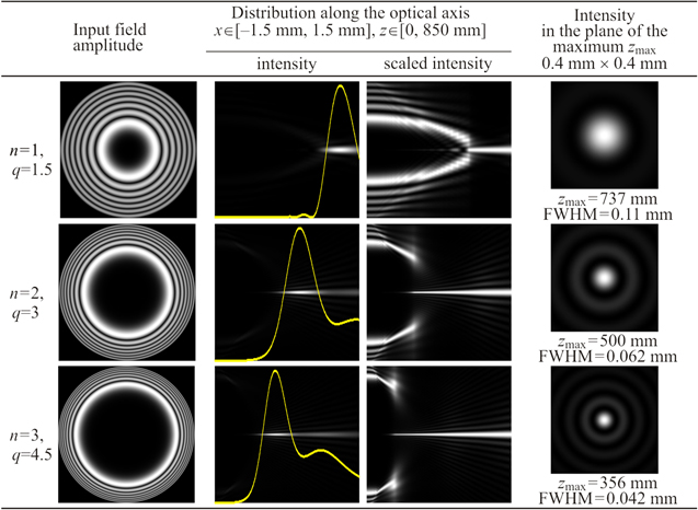
Figure 1. Modelling results for autofocusing beams formed by the Airy functions with superlinear argument described by equation (1).
Download figure:
Standard image High-resolution imageAccording to the results shown in figure 1, the increase of power n of the Airy function (when other parameters are not changed) leads to an increasing frequency nonlinearity of rings in the input field and their concentration at the peripheral part of the aperture. In fact, this means a growth of the NA defined by equation (4) of the optical element produces an autofocusing beam. Due to this, the maximum intensity value (focus) is formed closer to the input plane, while the transverse size of the focal spot (full width at half maximum, FWHM) decreases.
The scaled intensity patterns confirm the theoretical calculations in the previous section. In particular, it is clearly seen that when n > 1, the off-axis caustic does not reach the optical axis and the focus is formed on the axis suddenly and 'unexpectedly'. Nevertheless, it is possible to predict this distance using equation (21), if the parameters of the chirp beams are defined.
Using the approximation described by equation (2), the results of the sinusoidal functions with the selected parameters r0 и α0 are shown in figure 2.
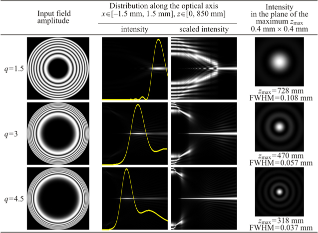
Figure 2. Modelling results for autofocusing beams formed by the three-parametric chirp-beams described by equation (2).
Download figure:
Standard image High-resolution imageComparing figures 1 and 2, there is a very close correspondence between Airy beams described by equation (1) and chirp beams described by equation (2), except that the focus is formed slightly closer to the input plane in the latter. This is due to the high-frequency rings having a larger amplitude in sin-functions, in comparison with Airy functions, which increases the numerical aperture of such an optical element.
For q = 1.5, the following values of parameters r0 = 0.5 mm and α0 = 0.000 53 were used in equation (16), which correspond to the numerical aperture NA = 0.0022 calculated by equation (22). The position of the focal distance zfoc = 709 mm defined by equation (20) is slightly lower than the numerically obtained value of 728 mm. Parameters r0 = 0.65 mm and α0 = 0.000 215 were used for q = 3, which correspond to the numerical aperture NA = 0.005. In this case, the position of the focal distance zmax = 441 mm determined by equation (21) is slightly lower than the calculated value of 470 mm. Parameters r0 = 0.7 mm and α0 = 0.000 16 were used for q = 4.5, which correspond to NA = 0.0079 and zmax = 324 mm, quite close to the numerical value of 318 mm.
To demonstrate the sudden autofocusing of superlinear chirp beams in comparison with sublinear chirp beams, figure 3 shows the transverse distributions of the intensity at distances corresponding to z1 = 0.5zmax, z2 = 0.75zmax and z3 = zmax for the chirp beams from figure 2.
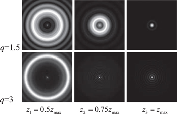
Figure 3. Calculated transverse intensity distributions (image size is  ) at different distances for q = 1.5 and q = 3.
Download figure:
Standard image High-resolution imageNote that by changing the parameter r0 (with relative change of the total radius), the focal distance is moved (as follows from equations (20) and (21)) without changing the numerical aperture of the optical element and the transverse size of the focal spot. The chirp order q defines the 'abruptness' of the focus appearing and its transverse dimension, and parameter α0 is an additional parameter for controlling of the autofocusing properties.
The use of superlinear chirp beams (q > 2) achieves similar effects using only two parameters q and α0 (r0 = 0), since the radial displacement is important only for 1 < q < 2.
Figure 4 demonstrates the comparative modelling results for sinusoidal functions described by equation (2) with p = 0, r0 = 0 and various values of q. Parameter α0 was chosen, taking into account a fixed number of rings in the input plane.
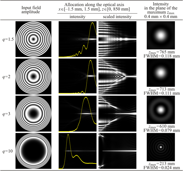
Figure 4. Modelling results for autofocusing beams formed by the two-parametric (r0 = 0) chirp-beams described by equation (2).
Download figure:
Standard image High-resolution imageThe value of q = 1.5 corresponds to the sublinear chirp, the value of q = 2 corresponds to the linear chirp, i.e. parabolic lens, values of q = 3 and q = 10 correspond to the superlinear chirp. Note that in the case 1 < q < 2, the absence of radial displacement does not achieve a clearly expressed focus (see figure 4, first line).
Parameter α0 = 0.000 416 was used for q = 1.5, which corresponds to the numerical aperture NA = 0.0018 according to equation (4). The focal position zmax = 750 mm determined by equation (15) is slightly lower than the numerical value equal to 765 mm. Parameter α0 = 0.000 242 was used for q = 2, which corresponds to NA = 0.0024 and the focal position zmax = 722 mm from equation (15) is slightly higher than the numerical value 713 mm. Parameter α0 = 0.000 142 was used for q = 3, which corresponds to NA = 0.0036 and the predicted focal position zmax = 606 mm is very close to the numerical value of 610 mm. Parameter α0 = 0.000 0668 was used for q = 10, which corresponds to NA = 0.0121 and the predicted focal position zmax = 250 mm is slightly higher than the numerical value of 213 mm.
Note that the estimate in equation (15) for large values q tends to the value zmax → 2R/NA, that corresponds to the double size of the shadow region.
From figure 4, the increasing q focus shifts closer to the input plane, similar to the three-parameter chirp beams considered above and the transverse size of focal spot decreases. However, if large values of q ≫ 1 are used, the autofocusing of the considered beams is more abrupt than for q < 2 (even when r0 ≠ 0). As predicted by the theoretical analysis, the off-axis caustic lines are almost parallel to the optical axis, but after a short distance, a sudden focusing takes place and a compact central focal spot is formed instead of the ring.
Thus, the results of numerical investigations of the three- and two-parametric chirp beams with the properties of sudden autofocusing fully confirm the analytical calculations obtained in the section 2.
4. Experiments
The optical scheme shown in figure 5 was used for the experimental investigation of circular superlinear chirp beams. The amplitude coding methods were used to transform the complex transmission functions given by equations (1), (2) and (16) to the pure phase profiles [20]. The spatial light modulator SLM (PLUTO-VIS, HOLOEYE, 1920 × 1080 pixels) was used for the experimental realisation of the phase profiles. The laser beam was collimated and expanded with the help of a combination of the micro objective MO, pinhole PH and the lens L1 directed on the display of SLM. A spatial filtering of the beam reflected from the modulator display was performed using a lens system L2, L3 and diaphragm D. The CCD video camera (UHCCD00800KPA, ToupCam, 1.67 μm pixel size) moving on the optical rail fixed intensity distributions for the beam at various distances from the plane z = 0 conjugated to the plane of the spatial light modulator display.
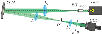
Figure 5. Optical scheme of experiments for studying the autofocusing properties of chirp-beams.
Download figure:
Standard image High-resolution imageFigure 6 shows the experimentally obtained intensity distributions of the nonlinear argument Airy beams described by equation (1) along the propagation axis (measures as a set of transverse distributions for z ∈ [0, 850 mm]). Beam parameters were matched with model beams shown in figure 1. Figure 6(a) shows that the classical circular Airy beam (n = 1) has an annular distribution that gradually narrows to form a focus. The experimentally measured values zmax = 765 mm and FWHM = 0.13 mm were somewhat larger than the numerical values (737 mm and 0.11 mm) due to a small defocusing of the incident beam.

Figure 6. Experimentally obtained intensity distributions of Airy beams, described by equation (1) along the propagation axis for different values of the power: (a) n = 1, (b) n = 2, (c) n = 3.
Download figure:
Standard image High-resolution imageFor Airy beams with a nonlinear dependence of the argument (n > 1), as seen in figures 6(b) and (c), the annular distribution 'smears' without reaching the optical axis. In this case, the intensity on the axis after the shadow region arises suddenly. As the power n increases, the focus position moves to the input plane and the focal spot transverse dimension decreases. The experimentally measured distance to the focus and the transverse size of the focal spot are as follows: for n = 2–zmax = 605 mm, FWHM = 0.08 mm; for n = 3–zmax = 495 mm, FWHM = 0.06 mm. Some increase in the experimental characteristics was due to a small defocusing of the incident beam.
A number of experiments were conducted to demonstrate the similar properties of chirp beams formed using optical elements matched with function described by equation (2). In this case, the beam parameters were not consistent with the numerical modelling, because the goal was to only demonstrate the qualitative effects. The results of two-parametric beams (r0 = 0) are shown in figure 7.

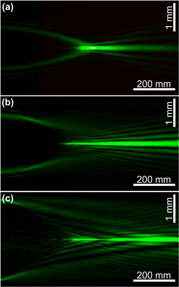
Figure 7. Experimentally obtained intensity distribution of two-parametric (r0 = 0) chirp-beams described by equation (2) along the propagation axis for different values of chirp order: (a) q = 1.5, (b) q = 3, (c) q = 10.
Download figure:
Standard image High-resolution imageIt is clearly seen in figure 7(a) that for q = 1.5 (sublinear chirp), the focus is formed rather gradually than abruptly. At the same time, for q = 3 and q = 10 (superlinear chirp, figures 7(b) and (c)), there is a sudden appearance of the intensity on the optical axis after the shadow region. Moreover, the focus position moves to the input plane with increasing chirp order and the transverse focal spot size decreases. In particular, the experimentally measured distance to the focus and the transverse size of the focal spot are as follows: for q = 1.5–zmax = 487 mm, FWHM = 0.07 mm; for q = 3–zmax = 465 mm, FWHM = 0.056 mm; for q = 10–zmax = 325 mm, FWHM = 0.041 mm.
The additional parameter of radial displacement r0 allows the expansion of the range of configurations of autofocusing beams and the possibility of focusing control. The experimental results for three-parameter beams described by equation (2) are shown in figure 8. It is seen, that in the case r0 ≠ 0 for q = 1.5 (sublinear chirp), the focus is at the distance of a crossing of the off-axis caustics with the optical axis. For q = 3 and q = 10 (superlinear chirp, figures 8(b) and (c)), the off-axis caustics do not reach the axis as the theory predicts, but intensity suddenly arises after the shadow segment on the optical axis.
Figure 8. Experimentally obtained intensity distribution of three-parametric chirp-beams described by equation (2) along the propagation axis for different values of the chirp order: (a) q = 1.5, (b) q = 3, (c) q = 10.
Download figure:
Standard image High-resolution image
By varying three parameters α0, the chirp order q and radial displacement r0, it is possible to achieve a situation when the focus is formed approximately at the same distance, but with a smaller transverse dimension of the focal spot, as demonstrated in figures 8(b) and (c).
In particular, the experimentally measured distance to the focus and the transverse dimension of the focal spot are as follows: for q = 1.5–zmax = 440 mm, FWHM = 0.058 mm; for q = 3–zmax = 355 mm, FWHM = 0.049 mm; for q = 10–zmax = 354 mm, FWHM = 0.037 mm.
Thus, the main effects that have been theoretically and numerically investigated in the previous sections are experimentally confirmed. Furthermore, the possibility of the effective control of autofocusing properties based on the considered two- and three-parameter chirp beams was demonstrated.
5. Conclusion
This work considered circular superlinear chirp beams, which provide faster and more abrupt autofocusing than circular Airy beams, theoretically investigating two- and three-parameter chirp beams with controlled autofocusing properties. The numerical simulations confirmed the theoretical expectations, demonstrating that the use of the considered parameters α0 (corresponds to the numerical aperture), chirp order q (determines the caustic path and focal lines type), and radial displacement r0 (also leads to a focus shift) allows the effective control of a wide range of autofocusing properties of circular beams. Furthermore, the experimental results showed good agreement with the theoretical analysis, demonstrating the convenience of using circular superlinear chirp beams for changing such autofocusing characteristics as the focus distance, its extent, abruptness of focusing and transverse size of the focal spot.
Acknowledgments
The work was funded by the Russian Federation Ministry of Education and Science of state-assigned task No. 3.5319.2017/8.9.