


ABSTRACT
In this study, we test the flux rope paradigm by performing a "blind" reconstruction of the magnetic field structure of a simulated interplanetary coronal mass ejection (ICME). The ICME is the result of a magnetohydrodynamic numerical simulation and does not exhibit much magnetic twist, but appears to have some characteristics of a magnetic cloud, due to a writhe in the magnetic field lines. We use the Grad–Shafranov technique with simulated spacecraft measurements at two different distances and compare the reconstructed magnetic field with that of the ICME in the simulation. While the reconstructed magnetic field is similar to the simulated one as seen in two dimensions, it yields a helically twisted magnetic field in three dimensions. To further verify the results, we perform the reconstruction at three different position angles at every distance point, and all results are found to be in agreement. This work demonstrates that the current paradigm of associating magnetic clouds with flux ropes may have to be revised.
Export citation and abstract BibTeX RIS
1. INTRODUCTION
Magnetic clouds (MCs), which represent about one-third of interplanetary coronal mass ejections (ICMEs), are defined as plasma structures with a size of ∼0.25 AU at 1 AU, characterized by a strong, and smoothly rotating magnetic field in a plasma of low proton temperature, and low plasma beta (Burlaga et al. 1981). If radially expanding, they exhibit a decreasing speed throughout the cloud. Other characteristics which many MCs have, such as specific charge states of heavy ions and bi-directionally streaming suprathermal (few 100s eV) electrons, especially, show that many MCs are composed of field lines connected at both ends to the Sun (Zurbuchen & Richardson 2006). To explain the characteristics of MCs, it was proposed more than 30 years ago that they consist of twisted flux ropes (Burlaga et al. 1981), and they have been described as such since then.
Numerical simulations have shown that a flux rope expanding from the solar surface will evolve during its propagation into an MC with all required plasma characteristics (Manchester et al. 2004; Roussev et al. 2003). Furthermore, Jacobs et al. (2009) successfully simulated a CME with typical characteristics of an MC, but without an underlying helical flux rope structure; the magnetic field structure had significant writhe, which explained the smooth rotation of the magnetic field lines. Here, we use writhe to indicate that there is a field rotation but the individual field lines are not twisted, in a way similar to what happens in the corona (e.g., see Török et al. 2010).
Under certain assumptions, it is possible to reconstruct the three-dimensional (3D) magnetic field configuration of an ICME from satellite observations; the main techniques are force-free reconstruction (Lepping et al. 1990; Lynch et al. 2003); magnetostatic reconstruction, referred as Grad–Shafranov (GS; Hu & Sonnerup 2001; Möstl et al. 2009a), torus reconstruction (Marubashi & Lepping 2007); and elliptical non-force free (Hidalgo et al. 2002). These reconstructions have been tested using 2.5-dimensional (2.5D) magnetohydrodynamic simulations in Riley et al. (2004). There, the authors found that the reconstruction and fitting methods have rather small errors concerning the axis orientation when the spacecraft passes close to the axis of the cloud. This conclusion was recently confirmed by a study by Vandas et al. (2010). Typically, it is expected that an MC has the lowest amount of twist at its center and the largest amount of twist at its boundaries. Using near relativistic electrons as a probing tool, Larson et al. (1997) analyzed the magnetic field line length at 1 AU for a well-observed MC and they found that the field lines length (and therefore the twist) was indeed minimal in the center and maximal at the boundaries.
Recent observations have put into question the association of all MCs with twisted flux ropes. In an extension of the study by Larson et al. (1997), Kahler et al. (2011), on the contrary, found that some MCs have constant field lines lengths throughout their cross section (irrespective of distance from the axis). In a study by Möstl et al. (2009a), the reconstructed flux rope was found to have a nearly constant amount of twist throughout the rope cross section. Finally, Farrugia et al. (2011) recently analyzed an ICME observed by Wind and the two STEREO spacecraft in 2007 November. They performed three reconstructions using measurements from the different spacecraft and the directions of the ICME axis were not in agreement with one another. In this article, we study how an ICME without a twisted flux rope is reconstructed based on simulated in-situ data. In Section 2, we give a brief overview of the simulation of Jacobs et al. (2009) and of the GS technique used to reconstruct the ICME. In Section 3, we present the results of our study and discuss the implication to the magnetic structures of MCs and ICMEs. Final conclusions are drawn in Section 4.
2. DATA AND METHODS
2.1. Simulations
The simulations we use are based on a model of solar eruption proposed by Roussev et al. (2007), where flux emergence and shearing motions at the Sun are mimicked to produce an eruption with minimal twist, but with a succession of writhed field lines. Here, we quickly summarize the main mechanism of the ejection and the associated creation of the writhed magnetic field lines. We study two different magnetic configurations, where the active region is composed of four magnetic charges of alternating polarity, positioned symmetrically around the solar equator. The active region is embedded in a simple dipole field. Depending on the orientation of the global dipole field, a dipolar or a quadrupolar active region is obtained, where the latter has the more complex magnetic topology.
As shown in Manchester (2007), for example, the emergence of a flux rope is often associated with shearing motions. To reproduce this, the two inner sources of the active region are subjected to shearing motions while moving along the inner neutral line. This energizes the magnetic field, disturbing the initial equilibrium. Consequently, closed loops rise and expand until the system reaches the point of loss of equilibrium, when magnetic reconnection results in an eruption of the sheared field. Although the driving mechanism is exactly the same in both simulations, the more complex quadrupolar case will result in a faster eruption (Jacobs & Poedts 2011).
In other numerical studies of CME initiation, rotating motions are applied in the active region, resulting in the eruption of a twisted flux rope (e.g., see Lynch et al. 2008). Here, there is no twist added into the system. However, through a series of reconnection events between the erupting magnetic field and the global dipole, the magnetic field of the CME shows a significant writhe. The magnetic tension force, on the other hand, will tend to rotate the writhed field lines. This results in a magnetic field possessing the signatures of an MC, but without containing a flux rope structure. Both the quadrupolar and dipolar simulations show this peculiarity (see Figure 1). For both simulations, synthetic satellite measurements were made at 15 R☉. Additionally, for the quadrupole case, another measurement was made at 70 R☉. Figure 2 shows the time evolution of the plasma variables as measured by the satellite positioned at 15 R☉ for the dipole (left) and quadrupole (right) cases. The position of the shock and the boundaries of the MC used for the reconstruction are marked by vertical lines. In what follows, we analyze these satellite measurements to see how this type of eruption would be interpreted in real satellite measurements.
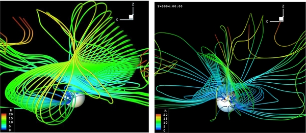
Figure 1. 3D views of the MC magnetic field structure at t = 4 hr shows the writhe in the magnetic field topology for the quadrupolar (left) and dipolar cases (right). Color code represents the radial distance from the Sun. The figure on the left was published in Jacobs et al. (2009) and is reproduced by permission of the AAS.
Download figure:
Standard image High-resolution image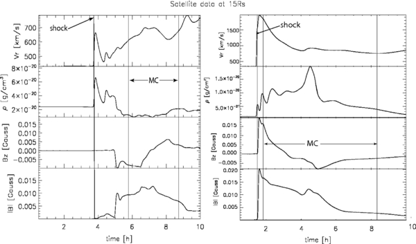
Figure 2. Synthetic satellite measurements for the dipolar (left) and quadrupolar (right) cases at 15 R☉ showing, from top to bottom, the radial velocity, mass density, magnetic field z-component and strength, and the magnetic cloud boundaries as chosen by the GS code.
Download figure:
Standard image High-resolution image2.2. Grad–Shafranov Magnetic Field Reconstruction Code
We start from synthetic satellite files of the plasma properties of a simulated magnetic ejecta taken from the simulation of Jacobs et al. (2009). The magnetic field configuration inside the magnetic ejecta is reconstructed from the time series; this is done using the GS magnetic field reconstruction code from Hu & Sonnerup (2002). This is based on magnetohydrostatic equilibrium of a system with an invariant direction and is a solution for what is basically a numerical boundary problem. It is assumed that the structure is time-invariant as it passes over the synthetic spacecraft, therefore the time series is equivalent to a one-dimensional (1D) boundary condition. It is further assumed that the reconstructed magnetic structure is invariant along the cloud axis, making the problem 2.5D. This is required to solve a 3D equation only with a 1D boundary condition, and it is an assumption also made in all other reconstruction codes.
For a 2.5D structure (invariant along z), the force balance,

can be reduced to the GS equation
where A is the magnetic vector potential, jz is the current density along the cloud axis, and Pt is the transverse pressure defined as Pt = p + B2z/(2μ0), with p being the thermal pressure. The first step to solve this equation is to determine the invariant axis, z. This is done by finding a frame in which the transverse pressure is a single value function of the magnetic vector potential (as shown in Figure 3). Then, the GS equation can be solved numerically (for details see Hu & Sonnerup 2002 or Möstl et al. 2009a).

Figure 3. Left panel: 2D view of the recovered magnetic field from the GS code for the simulation of the dipolar case at a distance of 15 R☉, with the Sun being to the right of the figure. Color code shows the strength of the magnetic field axial component, the black contours are lines of the transverse magnetic field in the paper plane, and the white contour is the MC boundary. The yellow and green arrows are the magnetic and velocity vectors along the spacecraft trajectory, respectively. Right panel: Pt(A) function fitting curve.
Download figure:
Standard image High-resolution image3. RESULTS
3.1. Reconstruction in the Direction of Propagation of the Ejection
Figure 3 demonstrates the reconstructed magnetic field topology in the ejecta for the dipole case. The cloud axis has an orientation of 109° longitude and −6 45 latitude, almost purely east–west in the ecliptic. Here, longitude and latitude refer to the angle between the cloud axis and the Sun–spacecraft line and the angle between the cloud axis and the ecliptic, respectively. The results of the GS procedure are similar to a typical MC observed in situ (see, for example, reconstructions in Möstl et al. 2008, 2009a). The reconstruction is consistent with a circular cross section MC with minimum distortion, which is what would be expected relatively close to the Sun for a twisted flux rope.
Figure 4 describes the reconstructed magnetic field topology in the MC from the simulation for the quadrupolar case where the synthetic satellite is at 15 R☉ (top row) and 70 R☉ (bottom row) at three different angular positions; the left column shows the reconstruction along the direction of the CME propagation. For the synthetic spacecraft at a distance of 15 R☉, the reconstructed cloud has the orientation of 704 longitude and −134 latitude (top left panel). This is a slightly different result to what was found in Jacobs et al. (2009), because here we use the GS reconstruction technique, whereas Jacobs et al. (2009) used a minimum variance analysis. For the synthetic satellite at a distance of 70 R☉, the bottom left panel of Figure 4 shows the recovered magnetic field from the GS code in the plane perpendicular to the cloud axis. The reconstructed cloud has the orientation of 956 longitude and −99 latitude.

Figure 4. Top row: same as the left panel of Figure 3, but for the quadrupolar case at a distance of 15 R☉ for (1) spacecraft along the direction of propagation of the ejection (left) and (2) ±30° away (middle and right), with the Sun to the right of the figures. Bottom row: same as the top row but for a spacecraft at a distance of 70 R☉.
Download figure:
Standard image High-resolution image3.2. Reconstruction Away from the Direction of Propagation of the Ejection
It is interesting to look at the magnetic field reconstruction from synthetic satellite data at different locations in the heliosphere. We perform the reconstruction of the MC for a satellite in the ecliptic, but with an angular separation of ±75 from the direction of propagation of the ejecta for the dipole case and with the separation of ±30° for the quadrupole case. In the middle and right column of Figure 4, we show the cases for the separation of 30° and the heliocentric distance of 15 and 70 R☉, respectively.
The top middle panel is for the synthetic satellite 30° away from the direction of propagation of the ejection (west 30) at a distance of 15 R☉. The reconstructed cloud has an orientation of 121° longitude and −50 latitude. The top right panel is for the synthetic satellite −30° away from the direction of propagation of the ejection (east 30) at the same distance. The reconstructed cloud has an orientation of 619 longitude and −79 latitude. It is important to compare the results of the three reconstructions with each other, recreating the case of multi-spacecraft observations. Multi-spacecraft observations eliminate the ambiguity caused by single satellite observations (Liu et al. 2008; Möstl et al. 2008, 2009b). The magnetic topology and field strength of the three reconstructions for the spacecraft at ±30° are consistent with each other and the directions of the reconstructed axes point toward a twisted flux tube anchored at the Sun, which is one of the most common interpretations of flux ropes (Burlaga et al. 1981; Chen 1996). In addition, all three reconstructions point toward an MC with a small inclination to the ecliptic. The reconstruction of the top right panel of Figure 4 is not totally consistent with this picture because of the different MC shape and slightly off-axis direction.
The bottom middle panel is for the synthetic satellite at west 30 at a distance of 70 R☉, and the reconstructed cloud has an orientation of 866 longitude and −48 latitude. The bottom right panel is for the synthetic satellite east 30, and the reconstructed cloud has an orientation of 814 longitude and −79 latitude. At this larger distance from the Sun, the simulation without twist still yields in-situ measurements which can be reconstructed as an MC from all three vantage points. In addition, all three reconstructions point toward an MC whose cross section is slightly elongated (expanding MC) and with a small inclination with respect to the ecliptic. The similar aspect of the cross section appears to validate the approximation of invariance along the cloud axis. The axis direction is approximately 90° from the satellite path at all three positions, which points toward a circular flux tube whose center is the Sun. This is another common interpretation for wide CMEs (Vourlidas & Howard 2006). Little is known on how the "radius of curvature" of an MC changes with distance from the Sun (see, for example, Lugaz et al. 2010). We found here that an MC becomes less curved as it expands and interacts with the background wind, which appears very reasonable.
Not shown here is the reconstructed magnetic field for synthetic satellites ±75 away from the direction of propagation of the ejection for the dipole case. We find that the axis of the reconstructed cloud has the orientation of 705 longitude and −60 latitude for the +75 case and 1118 longitude and −102 latitude for the −75 case. All three reconstructions have approximately the same shape, namely, that of a relatively circular cross section (as in the left panel of Figure 3). The direction of the axis as reconstructed from the three synthetic satellites is consistent with a twisted flux rope anchored at the Sun.
3.3. Comparison with the 3D Simulation
We can compare the reconstructed magnetic field in the plane perpendicular to the MC axis with the two-dimensional (2D) magnetic topology from the simulation as shown in Figure 5. This figure shows the magnetic field strength and magnetic topology of the eruption as seen in 2D cuts at heliocentric distances of 15 R☉ (left) and 70 R☉ (right) for the quadrupole case. Comparing the top row of Figure 4 and the left panel of Figure 5, there is a close match between simulated and reconstructed cloud. This is true for the elongated shape, the strength of the axial magnetic field (close to 1200 nT at its maximum), the extent of the cloud (0.04–0.06 AU in the direction perpendicular to the satellite's trajectory), as well as helicity sign (S-N cloud). Comparing the results at 70 R☉ (bottom left panel of Figure 4 and right panel of Figure 5), we find similar agreement. In particular, the extent of the cloud is about 0.1–0.2 AU and the maximum axial field strength about 70–80 nT in the reconstructed magnetic field as well as the simulated one. This proves that the GS code is very good at reconstructing the 2D magnetic topology of the ejecta, at least when the ejecta passes over the satellite in a plane containing the cloud axis as found in Riley et al. (2004). This is especially true considering that the 2D cuts from the simulation are "snapshots" at given times of the magnetic topology of the cloud, whereas the GS reconstruction are from a time series. However, the conclusion is very different when we compare our reconstruction as twisted flux tube whose cross section is shown in Figure 4 with the simulated 3D topology of the ejection shown in Figure 1. This shows that, although the GS code reconstructs the 2D magnetic topology very well, the typical conclusion that it comes from a twisted flux rope is not necessarily correct. Here, we demonstrate that the presence of writhed magnetic field can be the cause for such discrepancy between 2D reconstruction and 3D magnetic topology.

Figure 5. Left: a 2D view of the simulation for the quadrupolar case in approximately the same plane as the top right panel of Figure 4 at 15 R☉. The satellite position is marked with a purple circle. The color code shows the axial magnetic field strength while the black streamtraces illustrate the 2D projection of the magnetic field with the Sun to the right of the figure at (0,0). Right: same as in left frame, but at 70 R☉ to compare to the bottom right panel of Figure 4.
Download figure:
Standard image High-resolution image
4. SUMMARY AND CONCLUSIONS
In this study, we have investigated the magnetic field topology of MCs by reconstructing the magnetic field of two different simulated ICMEs using the GS reconstruction method. The magnetic fields in the simulated ICMEs have significant writhe, but very little twist. The reconstruction was performed at different distances and angular separations. By creating a scenario of multi-spacecraft observations, we have been able to remove the ambiguity caused by reconstruction from a single satellite. This presents a direct test to the code and provides robust results. For each of these multi-spacecraft scenarios, the cloud axes as reconstructed are consistent with each other and descriptive of a typical MC shape. The cross section of the reconstructed MC is in good agreement with 2D cuts from the 3D simulation. However, the reconstructed magnetic field of simulated ICMEs yields a helically twisted magnetic field, which is believed to be the typical structure of MCs. This is due to the assumption of invariance of the plasma properties along the axis of the MC. This assumption is required to perform any reconstruction but needs to be further improved. Here, we have demonstrated how, under this assumption, even magnetic fields with significant writhe and with little twist would be reconstructed as a twisted flux rope from in-situ measurements.
Because the synthetic satellite data in our study are taken closer to the Sun than 1 AU, the ICMEs still have a relatively strong expansion. In addition, the dipolar case shows a relatively unusual time variation for the radial velocity with contraction followed by expansion (see left panels of Figures 2 and 3). Gulisano et al. (2007) have shown that, when the cloud passes by a spacecraft close to its axis, as is the case for some of the reconstructions here, the error due to the expansion of the cloud is relatively small. It is our intention to look at models which take into account MC expansion in a follow-up study. We believe including the effect of expansion would not alter the magnetic field topology of the MC, but merely results in different shape of the cross section and orientation of the axis.
Here we introduce a novel case where a simulated MC which has writhed magnetic field could fulfill the model of magnetic twist, in spite of the different topology of the magnetic field lines. This "writhed" MC could not be detected as such by the magnetic field reconstruction codes that are designed to detect magnetic twist only. A magnetic field topology of significant writhe and very little twist can adequately explain the in-situ properties of MCs too, and is accordingly a model for magnetic field structure in MCs. Therefore, the current paradigm of automatically associating MCs with twisted flux ropes has to be revised.
Additionally, we have found that having multi-spacecraft measurements in a plane containing the reconstructed cloud axis does not allow distinction between writhe and twist. In further studies, we will look at reconstruction from satellite positions above or below the cloud axis. With numerical studies such as this one and careful analyses of actual multi-spacecraft measurements, it might be possible in the future to distinguish between writhed and twisted magnetic field in ICMEs.
The authors wish to thank the reviewer for his/her useful comments, and pray that God protects researchers from Baba Yaga. This research was supported by the grants NNX07AC13G, ATM06-39335, NNX08AQ16G, GOA/2009-009, FP7/2007-2013, Austrian Science Fund (FWF): [P20145-N16], and NAS5-0313.