


ABSTRACT
The nature of small-scale turbulent fluctuations in the solar wind is investigated using a comparison of Cluster magnetic and electric field measurements to predictions arising from models consisting of either kinetic Alfvén waves or whistler waves. The electric and magnetic field properties of these waves from linear theory are used to construct spacecraft-frame frequency spectra of (|δE|/|δB|)s/c and (|δB∥|/|δB|)s/c, allowing for a direct comparison to spacecraft data. The measured properties of the small-scale turbulent fluctuations, found to be inconsistent with the whistler wave model, agree well with the prediction of a spectrum of kinetic Alfvén waves with nearly perpendicular wavevectors.
Export citation and abstract BibTeX RIS
1. INTRODUCTION
Magnetized plasma turbulence plays an important role in regulating the transport of energy in space and astrophysical plasmas. The dissipation of the turbulence leads to heating of the plasma medium, and the development of a predictive theory of this plasma heating is essential to the interpretation of observations of many astronomical systems, from galaxy clusters to black hole accretion disks to the interstellar medium filling our Galaxy (e.g., Schekochihin et al. 2009 and references therein). The solar wind provides a unique environment in which spacecraft can directly measure the turbulent fluctuations at the small scales on which the turbulence is dissipated, providing the detail necessary to identify the nature of these small-scale fluctuations, information critical for unraveling the physical mechanisms by the which the turbulence is dissipated.
The nature of the dissipation range fluctuations of solar wind turbulence remains a major open question in heliospheric physics. The two leading hypotheses are that these fluctuations have the characteristics of kinetic Alfvén waves (Leamon et al. 1998a, 2000; Howes et al. 2008a; Schekochihin et al. 2009) or of whistler waves (Stawicki et al. 2001; Krishan & Mahajan 2004; Galtier 2006; Gary & Smith 2009; Saito et al. 2010; Podesta et al. 2010; Shaikh 2010), although a number of other possibilities have been discussed, including ion cyclotron waves (Goldstein et al. 1994; Leamon et al. 1998b; Gary 1999; He et al. 2011), ion Bernstein waves (Howes 2009; Sahraoui et al. 2011), or that the fluctuations are not wave-like at all, but correspond instead to nonlinear structures, such as current sheets (Sundkvist et al. 2007; Osman et al. 2011).
That the nature of the dissipation range fluctuations remains uncertain, even though we can measure the fluctuations directly, is due primarily to three reasons: (1) in situ measurements of solar wind turbulence are made at only one or a few points in space, (2) the measurements are made in the frame of reference of the spacecraft, a frame typically moving at a super-Alfvénic velocity relative to the plasma rest frame, and (3) the measurements are often made close to the limits of instrument capabilities. For single-point spacecraft measurements, it is not possible to uniquely separate the fluctuations due to the sweeping of spatial structure past the spacecraft from temporal fluctuations in the plasma frame. One can, however, determine the fluctuations that would be measured in the spacecraft frame for a particular model of the turbulent fluctuations in the plasma frame. This theoretical prediction may then be compared directly to spacecraft measurements to determine the nature of the small-scale turbulent fluctuations.
In this Letter, we evaluate whether the small-scale turbulent fluctuations measured in the solar wind have characteristics similar to kinetic Alfvén waves or whistler waves, the two leading hypotheses. Electric and magnetic field measurements from the Cluster spacecraft are compared to theoretical predictions of the properties of the fluctuations measured in the spacecraft frame due to two models: a spectrum of kinetic Alfvén waves and a spectrum of whistler waves. The linear eigenfunctions of these two waves are used to construct the spacecraft-frame frequency spectra of two quantities: the ratio of the electric to the magnetic field (|δE|/|δB|)s/c and the normalized parallel magnetic field fluctuations (|δB∥|/|δB|)s/c. The analysis in this Letter provides new evidence that the measurements are inconsistent with the whistler turbulence model but agree well with the model of a cascade of kinetic Alfvén wave turbulence.
2. MEASUREMENTS
We use measurements from the electric field and waves (EFW; Gustafsson et al. 1997), fluxgate magnetometer (FGM; Balogh et al. 1997), Cluster ion spectrometer (CIS; Reme et al. 1997), and plasma electron and current experiment (PEACE; Johnstone et al. 1997) instruments on board the Cluster spacecraft in the unperturbed solar wind at 1 AU during the interval 03:00:00–04:42:00 UT on 2003 January 30. The electric field and magnetic field data are from Cluster 4 at 19.50 RE, while plasma data are taken from Cluster 3 at 19.35 RE.
We use the geocentric solar ecliptic (GSE) Y electric field Ey from EFW (Gustafsson et al. 1997), sampled at 25 Hz, for all of our electric field analysis because this component tends to have the lowest noise level, as explained in Bale et al. (2005). The FGM instrument (Balogh et al. 1997) yields three-component magnetic field vectors sampled at 22 Hz. Since we analyze only the y-component of the electric field, Ey, we focus here on the Bz component of the magnetic field, because this component is related to Ey and Vpx (velocity component along the radial direction) through the Lorentz transformation (Bale et al. 2005). Moments of the solar wind ion distribution (density, velocity, and temperature) are computed from the CIS instrument (Reme et al. 1997), and the electron temperature is computed from the electron spectrum measured by the PEACE instrument (Johnstone et al. 1997).
Figure 1 shows an overview of the Cluster data used for the analysis presented here, with vector data presented in the GSE coordinate system: (1) the radial (GSE X) component of the solar wind proton velocity, Vpx; (2) the remaining components of the solar wind velocity, Vpy and Vpz; (3) the proton density, Np; (4) the proton and electron temperatures, Tp and Te; (5) all three components of the magnetic field, Bx, By, and Bz; (6) two components of the electric field, Ex and Ey; and (7) the proton plasma beta, βp. The average solar wind parameters for this interval are Np = 9 cm−3, solar wind speed Vsw = 427 km s−1, Tp = 13.6 eV, Tp, ⊥/Tp, ∥ ∼ 0.9–1, and Te = 13.0 eV, proton thermal speed vthi = (Tp/mp)1/2 = 36.1 km s−1, magnetic field strength |B| = 11 nT, Alfvén speed vA = 78.1 km s−1, and the proton plasma βp = 0.4. The average angle θVB between  and
and  is 118°. The proton and electron cyclotron frequencies are fci = 0.16 Hz and fce = 302.5 Hz. Our analysis includes data from 03:00:00 to 04:42:00 UT, where the solid black vertical line in Figure 1 indicates the end of our interval, excluding the sharp change in Bz and Ey. This interval used for analysis is ambient, unconnected, low-beta solar wind.
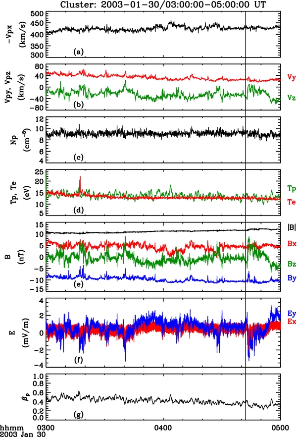
Figure 1. Cluster data over the interval 2003 January 30 03:00:00–05:00:00 UT: (a) solar wind velocity, Vpx; (b) solar wind velocity, Vpy and Vpz; (c) proton density, Np; (d) proton and electron temperatures, Tp and Te; (e) magnetic field, Bx, By and Bz; (f) electric field, Ex and Ey; and (g) proton plasma beta, βp.
Download figure:
Standard image High-resolution imageTo compute power spectra, the electric field Ey data at 25 Hz are sub-sampled onto the time tags of Bz at 22 Hz by linear interpolation; a total of exactly 217 points (≃ 99.3 minutes) are used. The power spectral density (PSD) is computed using both fast Fourier transform (FFT) and Morlet wavelet schemes.
Windowed Fourier transforms are used in which the data interval is divided into 4096 point (∼186 s) contiguous ensembles. We use a half-ensemble overlap in the windowing, so that the total number of ensembles is 2 × 217/4096 = 64, each with an inherent bandwidth of Δf ≃ 1/186 Hz. The final spectrum is computed as the average of the 64 ensembles. We find that the overlap used optimally minimizes the spectral variance at high frequencies close to the Nyquist frequency. Figure 2 shows the FFT power spectra of the z-component of the magnetic field Bz (black) the y-component of the electric field, Ey (red). The unprocessed Ey spectrum (red) clearly shows instrumental artifacts at the spacecraft spin frequency of 0.25 Hz and its harmonics. To remove the power in these spin-harmonic spikes, a finite impulse response filter is applied to the Fourier transformed data to notch out the primary perturbations; the notch-filtered Fourier spectrum for Ey (orange) is shown in Figure 2. The Ey spectrum (orange) also shows a broad bump around 1 Hz, believed to be interference from the WHISPER (Décréau et al. 1997) instrument on the Cluster spacecraft, and/or wake effects.
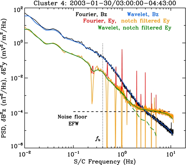
Figure 2. Magnetic and electric field FFT spectra for Bz (black), Ey (red), and notch-filtered Ey (orange). Wavelet spectra for Bz (blue), notch-filtered Ey (green solid), and noise-subtracted Ey (green dashed).
Download figure:
Standard image High-resolution imageWavelet spectra of Bz and of the notch-filtered Ey were also computed using 129 log-spaced frequencies, where the final wavelet PSD is computed as the square of the spectrum averaged over time. The wavelet PSD of Bz (blue) and of the notch-filtered Ey (solid green) are also shown in Figure 2. The FFT and the wavelet spectra agree remarkably well for both electric and magnetic fields, but the much larger bandwidth of the wavelet PSD leads to smooth averaging over the residual spin-harmonic dips in notch-filtered Ey.
Below the break frequency observed at fb ≃ 0.4 Hz in Figure 2, the electric and magnetic field spectra are well correlated (Bale et al. 2005; Chen et al. 2011). Fitting the frequency PSD to a power law, PSD∝f−α, this low-frequency range has α ≃ 1.65, consistent with the value α = 5/3 characteristic of the inertial range of plasma turbulence (e.g., Bale et al. 2005; Salem et al. 2009; Chen et al. 2011). In the dissipation range at higher frequencies f > fb, the magnetic spectrum steepens to α ≃ 3.3 up to 2 Hz, similar to values found in other high-frequency studies of the dissipation range (Smith et al. 2006; Sahraoui et al. 2009; Kiyani et al. 2009; Alexandrova et al. 2009; Chen et al. 2010a). While Bale et al. (2005) previously reported a flattening of the electric field spectrum in this frequency range scaling as α ≃ 1.26, the Ey spectrum here appears to steepen to α ≃ 2.9 from fb up to about 2 Hz. At higher frequencies, the Ey flattens significantly, which is probably due to noise in the EFW instrument.
We estimate the value of the EFW spectrum noise floor by identifying a "quiet" time interval (with a low level of electric fluctuation), for which the electric field spectrum is basically flat for f > 1 Hz, with a value of 1.2 × 10⁻⁴ mV2 m−2 Hz−1. This is significantly higher than the digitization noise of EFW. Subtracting this estimated EFW noise floor from the notch-filtered Ey wavelet spectrum (solid green), we obtain the "de-noised" Ey wavelet spectrum (dashed green) in Figure 2. We restrict our analysis here to f < 2 Hz, corresponding to the frequencies where the measured Ey spectrum is more than twice the estimated noise floor.
3. THEORETICAL PREDICTIONS
In this section, we construct theoretical predictions for the spacecraft-frame frequency spectra of the ratio of the electric to the magnetic field (|δE|/|δB|)s/c and of the normalized parallel magnetic field fluctuations (|δB∥|/|δB|)s/c for two models: (1) a spectrum of kinetic Alfvén waves and (2) a spectrum of whistler waves. Numerical simulations (Howes et al. 2011) show that the energy spectra of turbulent fluctuations in this range can be described well by linear theory.
The first step is to determine the linear eigenfunction (dispersion relation) of each wave in the plasma frame. For the kinetic Alfvén wave, we choose a limit of the two-fluid linear warm plasma dispersion relation for the Alfvén wave/kinetic Alfvén wave solution (Lysak & Lotko 1996; Stasiewicz et al. 2000), and, for the whistler wave, we use the cold plasma dispersion relation solution for the whistler wave (Swanson 2003; Sazhin 1993); comparison of these simplified linear solutions to a numerical solution of the Vlasov–Maxwell system (Quataert 1998; Howes et al. 2006) is given in a companion work (C. S. Salem et al. 2011, in preparation), where complete details on the calculation of this theoretical prediction are provided.
Assuming the non-relativistic conditions of the solar wind and Maxwellian equilibrium distribution functions, the plasma frame linear Vlasov–Maxwell eigenfunction solution depends on four parameters, ωVM(k, θ, βi, Ti/Te): wavevector magnitude k, the angle θ between the local mean magnetic field  and the wavevector
  , ion plasma beta βi, and ion-to-electron temperature ratio Ti/Te (Howes et al. 2006). Without loss of generality, we specify a coordinate system with the local mean field
  and the solar wind velocity
  in the x–z plane. An arbitrary wavevector is given by
  , where θ is polar angle with respect to
  and ϕ is azimuthal angle from the x-axis.
Single-point spacecraft measurements can be used to determine the angle θVB between  and
and  , but they do not constrain the direction of the wavevector, so the values of θ and ϕ must be provided by the model of the turbulent fluctuations. Assuming a uniform azimuthal distribution of wave power about the magnetic field, we average over the full 2π distribution in ϕ, leaving θ as a parameter that characterizes the model of the turbulent fluctuations.
For a single plane wave mode with wavevector  , the corresponding spacecraft-frame frequency of the fluctuations is computed using
  , accounting for the Doppler shift arising from the relative velocity
  between the solar wind plasma frame and the spacecraft frame. In addition, the electric and magnetic field fluctuations due to the wave are Lorentz transformed from the plasma frame to the spacecraft frame (C. S. Salem et al. 2011, in preparation), yielding the electric and magnetic fields in the spacecraft frame as a function of the spacecraft-frame frequency,
  and
and  , due to the plane wave mode with wavevector
  . These values are then averaged over the full 2π distribution in ϕ, as described above, to yield a prediction for the observed electromagnetic fields. The turbulent models under consideration span a range of values of wavenumber k at a chosen constant θ.
The results of the predicted values of (|δE|/|δB|)s/c for whistler waves (black/blue) and kinetic Alfvén waves (red) for various values of θ are presented in Figure 3. The observed ratio of (|δE|/|δB|)s/c ∼ |δEy|/|δBz| from the Cluster measurements of the magnetic and electric field spectra in Figure 2 are overplotted (green solid and dashed). The measurements are not consistent with the cold whistler predictions for angles of 0° or 30°. The kinetic Alfvén wave mode at nearly perpendicular wavevectors or the cold whistler mode at 70° or 89° appear to be consistent with the observations.
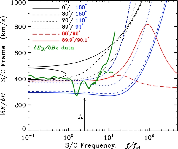
Figure 3. Prediction of |δE/δB|s/c for kinetic Alfvén waves (red curves) or whistler waves (black and blue curves) with specified angle θ. Cluster measurements of |δEy/δBz| up to 2 Hz, or 12fci, are presented without (green solid) and with (green dashed) the EFW noise floor removed.
Download figure:
Standard image High-resolution imageTo break the degeneracy between the two models, kinetic Alfvén waves or whistler waves, each with a spectrum of nearly perpendicular wavevectors, we may consider a measure of the compressibility of the fluctuations, the ratio of the parallel magnetic field fluctuation to the total magnetic field fluctuation, (|δB∥|/|δB|)s/c (Chaston et al. 2009; Gary & Smith 2009). We use the predicted magnetic field fluctuations transformed to the spacecraft frame to predict signature of (|δB∥|/|δB|)s/c for the two wave modes. This comparison leads to the results, presented in Figure 4, for cold whistlers (black/blue) and kinetic Alfvén waves (red). The results show very clearly that the measured parallel magnetic field fluctuations are inconsistent with the whistler wave for any angle of the wavevector. The results show remarkably good agreement with the prediction for the kinetic Alfvén wave with a nearly perpendicular wavevector.

Figure 4. Prediction of |δB∥|/|δB|s/c for kinetic Alfvén waves (red) or whistler waves (black/blue) with specified angle θ. Cluster FGM measurements up to 2 Hz, or 12fci, are shown in green.
Download figure:
Standard image High-resolution image
4. CONCLUSIONS
Here we present Cluster measurements of the spacecraft-frame frequency spectra of the ratio of the electric to the magnetic field (|δE|/|δB|)s/c and of the normalized parallel magnetic field fluctuations (|δB∥|/|δB|)s/c. Comparison to theoretical predictions of the spectra arising from a spectrum of kinetic Alfvén waves or whistler waves shows that only a kinetic Alfvén wave spectrum, with a nearly perpendicular wavevector power distribution, is consistent with the Cluster observations. This is consistent with theoretically proposed models for a solar wind dissipation range consisting of a critically balanced kinetic Alfvén wave cascade (Howes et al. 2008b, 2008a; Howes 2008; Schekochihin et al. 2009). This result also agrees with measurements of the wavevector anisotropy below ion scales, which show that the wavevectors remain at large angles to the magnetic field (Podesta 2009; Chen et al. 2010b; Sahraoui et al. 2010) in both field components (Chen et al. 2010a).
Previously, Sahraoui et al. (2009) found good agreement between |δEy|/|δBz| from Cluster measurements to the prediction for kinetic Alfvén waves, but due to the use of Taylor's hypothesis they could not show that the results were inconsistent with high-frequency whistler waves. Subsequently, using a multi-spacecraft k-filtering analysis, Sahraoui et al. (2010) found that rest-frame frequencies of the nearly perpendicular turbulent fluctuations were significantly lower than the frequencies of the fast magnetosonic mode, but the much lower kinetic Alfvén wave frequencies were below the error threshold of their measurements. Gary & Smith (2009) used a comparison of magnetic compressibility measurements to linear Vlasov–Maxwell theory predictions to argue for the presence of whistler mode fluctuations as well as kinetic Alfvén wave fluctuations (see also Podesta & Gary 2011). Other studies (Hamilton et al. 2008; Smith et al. 2012) based on the slab/2D model claim that the dissipation range has more k∥ wavevectors than k⊥. This Letter, however, presents two new tests that, together, directly demonstrate that the small-scale turbulent fluctuations in a low-beta solar wind interval consist of a spectrum of kinetic Alfvén wave turbulence.
It is possible that kinetic temperature anisotropy instabilities, which are seen to regulate the solar wind ion temperature anisotropy (e.g., Bale et al. 2009), may lead to the generation of other wave mode fluctuations in the dissipation range. In the low βp solar wind interval analyzed here, however, the plasma is sufficiently distant from instability thresholds for such mechanisms to be likely to contribute to the turbulent dynamics.
The authors thank Dr. M. Wilber for providing validated Cluster CIS moments and proton temperature anisotropy data used in this study. We also thank Professor A. Schekochihin for helpful discussions. This work was supported by NASA grants NNX10AC03G, NNX10AT09G and NNX09AE41G (Berkeley) and NNX10AC91G (Iowa), and by NSF grants AGS-0962726 (Berkeley) and AGS-1054061 (Iowa).