
Abstract
3D graphene foam is the main aim of this research work. Graphene foam is synthesized on the Ni-foam by the CVD technique. The graphene foam has been characterized by XRD, FESEM, Raman spectroscopy and BET techniques. The resistance of graphene foam with a variance of temperature has been measured through an LCR meter and has been analyzed with classical and neutrosophic analysis. As a result, it is seen that graphene foam is expressing both conductor and semiconductor electric properties and also it is observed that neutrosophic analysis is more flexible to analyze the resistance of graphene foam.
Export citation and abstract BibTeX RIS

Original content from this work may be used under the terms of the Creative Commons Attribution 4.0 licence. Any further distribution of this work must maintain attribution to the author(s) and the title of the work, journal citation and DOI.
1. Introduction
The development of flexible electronic circuits and devices has increased dramatically in recent years. Numerous nano-materials are used for this purpose like carbon containing-materials i.e. carbon nano-tubes (CNTs) and carbon nano-fibers, see (Zhang et al 2015) and (Dimchev et al 2010). Graphene is a chemically derived nanomaterial, which is an allotropic form of carbon with 2D hexagonal lattices and has zero band gaps, see (Geim & Novoselov, 2010). It has remarkable electric and conducting properties like it has 4 times larger electron mobility than III-V, see (Chen et al 2008). Numerous researchers have worked to connect 2D graphene with 3D structure materials by exploiting graphene foam, for remarkable electrical and thermal properties, which can be used in different applications, see (Geim 2009). Generally, it is seen that graphene foam is produced by chemical vapor deposition (CVD). The microcellular graphene foam based on Ni foam was fabricated with the help of ambient pressure CVD, which has a pore wall thickness of 5 nm (Jiang et al 2016). Similarly, the synthesization of 3D graphene foam with higher electrical conductivity of about 125 S cm−1 with a surface area of about 1625.4 cm g−1, was performed by plasma-enhanced CVD (Chen et al 2014). Also, CVD is used to fabricate the graphene foam based on Ni nanowires for high electric and mechanical properties (Min et al 2014). The reference (Jinlong et al 2017) used pitting pits Ni foam to fabricate the 3D graphene foam. They used NaCl solution to create pitting pits on the surface of Ni foam and deposited the graphene by CVD. The reference (Li et al 2015) developed the graphene foam through the graphene oxide (GO) on Ni foam and used it for sensing purposes. Also, different researchers have worked on graphene foams and got useful data of their electric, thermal as well as mechanical properties. The analysis of this data is a very caring task that is performed in form of tables as well as graphs through different methods like the classical analysis. More information can be seen in (Huang et al 2017).
Neutrosophic is a type of method used to analyze the data, which was introduced by Smarandache (Smarandache 2013). It is a reliable technique of statistics, which is the generalization of the fuzzy technique and is also more efficient. At the present time, the use of neutrosophic techniques is increased to analyze the data in several fields i.e. in medicine for diagnoses data measurement (Ye 2015), in applied sciences (Christianto et al 2020), in astrophysics i.e. earth speed (Aslam, 2021a), in humanistic (Smarandache 2010) and in material science (Afzal et al 2021, 2021). The neutrosophic technique is used on the interval point values data i.e. having indeterminacy, see (Aslam 2021b). This is a significant benefit over the classical techniques because classical statistics only deal with fixed point values data i.e. having no indeterminacy. Moreover, the neutrosophic technique is more helpful than classical techniques see the examples in the following references (Smarandache 2014, Chen et al 2017a, 2017b). Different statistical techniques were developed under neutrosophic statistics by Muhammad Aslam (Aslam 2020a, 2020b).
Present work reports the motive study of graphene foam resistance variance due to changes in temperature and current. Graphene foam is produced on the Ni foam surface through CVD and its structural, as well as morphological properties, are investigated with different characterization techniques. The resistance of the foam is measured with respect to the temperature as well as current and analyzed through neutrosophic as well as the classical analysis methods.
2. Experimental
For the fabrication of the GF, we have used porous nickel (pure 99.99%) foam of size about 25 × 25 mm as the template for graphene deposition as shown in figure 1. The Ni foam is first cleaned with the by sonication in acetone for 2 h, then put in DI water for 30 min and dried by oven at 100 °C for 5 h. The Chemical vapor deposition (CVD) technique with a decomposition of CH4 at 750 °C under ambient pressure has been used for the deposition of graphene on Ni foam. A hot FeCl3 solution has been used to remove the Ni and as a result, we have gotten the 3D graphene foam structure (Yavari et al 2011).

Figure 1. Graphene foam of size 23 × 23 mm.
Download figure:
Standard image High-resolution imageThen, we put this graphene foam on a clean glass slide for the characterization of structure, electric and surface properties. For structural properties XRD and for surface morphology FESEM techniques have been used. Raman spectroscope having a laser excitation with 488 nm wavelength has been used to observe the quality of 3D graphene foam. Similarly, to observe the adsorption of nitrogen gas on the surface area of 3D graphene foam the Brunauere-Emmette-Teller (BET) has been also used. The electric properties by measuring resistance are studied in the lab at room temperature. For measuring the resistance of the sample LCR meter has been used which is associated with a controlled chamber as shown in figure 2. Resistance is measured by varying the temperature and current, separately. All data has been collected in interval form i.e. at any specific value of temperature or current both maximum and minimum change in the value of resistance has been measured for analysis by both classical and neutrosophic approach.

Figure 2. Schematic diagram of characterization setup.
Download figure:
Standard image High-resolution image3. Result and discussion
XRD patterns of graphene foam can be seen in figure 3. All the peaks are satisfying the standard value. The first peak at 26.1° is expressing the presence of graphene. It is seen that the peak of graphene is shifted down slightly i.e. not much sharper, which is indicating that the interlayers of graphene with d002 spacing decrease based on Bragg's law, see (Ebrahimi et al 2019, Yang and Guo 2019). Similarly, (111) at 44.8°, (200) at 52.1° and (002) at 76.9° peaks are expressing the existence of the Ni foam.
The surface morphology of the graphene foam has been analyzed through field emission scanning electron microscopy (FESEM) as shown in figure 4(lift side). There are many black spots which are expressing the Ni foam and also 3D graphene structure on Ni foam can be easily seen. It is also observed that the morphology of the graphene is not changed and exhibits gauze morphology with wrinkles and ripples edge. It is assumed that wrinkles and ripples of graphene could be led to lower free energy in the system and avoid the graphene combinations to stabilize the graphene interlayers structure (Fasolino et al 2007).

Figure 3. XRD Pattern of graphene foam.
Download figure:
Standard image High-resolution image
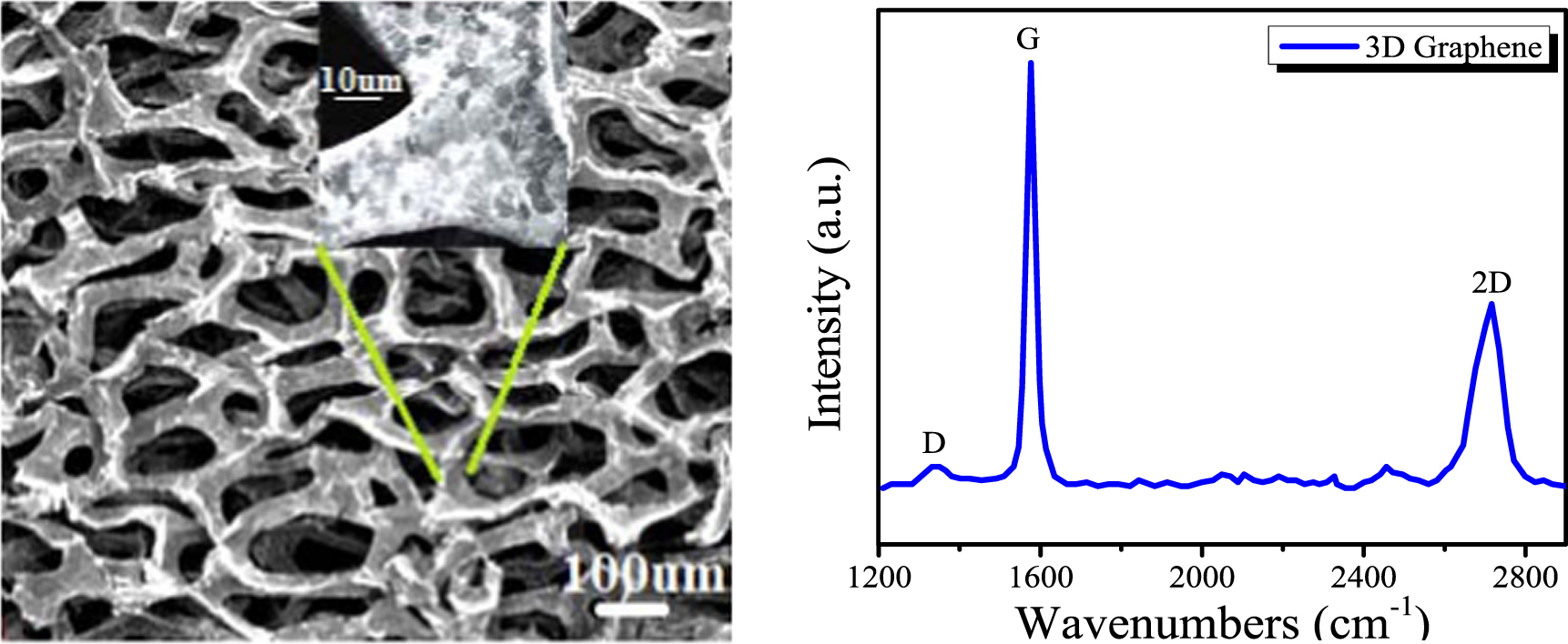
Figure 4. Lift side is the FESEM of the graphene foam on Ni foam and Right side is the Raman shift of the graphene foam.
Download figure:
Standard image High-resolution imageSimilarly, figure 4 (right side)is expressing the Raman spectroscopy spectrum. We have observed three peaks as D, G and 2D at the wavenumbers about 1370, 1591 and 2695 cm−1, respectively. The 'D' is a defect peak, which is highlighting the defects as well as disorders between layers of graphene. The 'G' is the characteristic peak of carbon structure sp2, which is highlighting the symmetry as well as the crystallization of graphene structure. Similarly, '2D' is a double-phonon-resonance peak, which is expressing the graphene stack degree i.e. identifying the presentence of graphene, see (Ferrari et al 2006, Qin et al 2022). We have used the BET technique to observe the specific surface area of the 3D graphene. We have calculated about 411.95 m2/g specific surface area of graphene foam. That is expressing the high porosity with a high surface area of the graphene foam. This means that graphene is very advantageous for contacting the electrodes materials, used in the electrochemical systems and electric layers for different devices like capacitors, see (Zhang and Zhao 2009, Yan et al 2019, Qi et al 2021) etc. One can also find the electrochemical impedance test using the EIS as expressed in the following reference (Yan et al 2022). But we have not added this work due to the unavailability of technique.

Figure 5. Graphs of resistance versus temperature for graphene foam.
Download figure:
Standard image High-resolution imageWe have fabricated the sample according to (Yavari et al 2011, Jiang et al 2016, Jinlong et al 2017) and we used an LCR meter to measure the electrical properties of the graphene foam. We noted that data is imprecise (i.e. it is in intervals) and reported the graphene foam measurement obtained from the LCR meter in table 1. For the data in the interval, neutrosophic statistics can be applied effectively as compared to classical statistics.
Table 1. Resistance measured data by changing temperature and current.
| Temperature | Resistance | Current | Resistance |
|---|---|---|---|
| (K) | (Ω) | (mA) | (Ω) |
| 292 | [3.025; 3.047] | 1 | [3.013, 3.025] |
| 296 | [3.010; 3.031] | 5 | [3.001, 3.009] |
| 301 | [2.998; 3.020] | 10 | [3.000, 3.008] |
| 305 | [2.992; 3.017] | 15 | [2.991, 3.010] |
| 309 | [2.980; 3.002] | 20 | [2.986, 3.001] |
| 315 | [2.971; 2.992] | 25 | [2.984, 2.995] |
| 319 | [2.981; 3.002] | 30 | [2.976, 2.992] |
| 323 | [2.975; 2.997] | 35 | [2.972, 2.988] |
| 328 | [2.967; 2.988] | 40 | [2.964, 2.983] |
| 331 | [2.971; 2.991] | 45 | [2,955, 2.971] |
| 335 | [2.967; 2.987] | 50 | [2.945, 2.966] |
| 339 | [2.957; 2.978] | 55 | [2.943, 2.952] |
| 345 | [2.935; 2.958] | 60 | [2.942, 2.961] |
| 353 | [2.925; 2.947] | 65 | [2.941, 2.956] |
| 360 | [2.914; 2.935] | 70 | [2.932, 2.946] |
| 366 | [2.912; 2.933] | 75 | [2.925, 2.936] |
| 375 | [2.903; 2.925] | 80 | [2.912, 2.936] |
| 378 | [2.891; 2.914] | 85 | [2.910, 2.926] |
| 383 | [2.892; 2.915] | 90 | [2.906, 2.918] |
| 388 | [2.895; 2.917] | 95 | [2.902, 2.920] |
| 393 | [2.891; 2.913] | 100 | [2.899, 2.916] |
| 398 | [2.880; 2.901] | 105 | [2.895, 2.913] |
| 405 | [2.859; 2.881] | 110 | [2.892, 2.908] |
| 412 | [2.857; 2.880] | 115 | [2.889, 2.902] |
| 419 | [2.844; 2.867] | 120 | [2.888, 2,901] |
| 426 | [2.841; 2.862] | 125 | [1.880, 2.895] |
| 431 | [2.830; 2.854] | 130 | [2.879, 2.893] |
| 435 | [2.837; 2.859] | 135 | [2.869, 2.888] |
| 449 | [2.820; 2.842] | 140 | [2.862, 2.883] |
From the above table 1, it is seen that the resistance of the graphene foam on Ni foam decrease with an increase in the temperature and current. This is because the graphene is a zero-gap semiconductor; the initial value of temperature resistance is a maximum but as the temperature increases the charge carrier's density also increases, so resistance starts to decrease. However, the resistance is not smoothly decreasing. Because for graphene foam the graphene is deposed on the Ni foam and Ni is a conductor in nature. Similarly, for current same thing happens. In short, the graphs are expressing the major semiconductor and minor conductor properties of the graphene foam.
3.1. Analysis of resistance of graphene foam
As already mentioned, we have performed two types of analysis i.e. classical and neutrosophic analysis. For the classical analysis, we take the average [(maximum value + minimum value)/2] of the interval to convert the interval value into a fix point value. For example, at 292 K temperature, we get [3.025; 3.047] Ω resistance interval. So, we convert it into a fix point value i.e. 3.036 Ω by taking its average. But for neutrosophic analyses, we have to first develop or modify the neutrosophic formula, so let us see the definition of neutrosophic.
Let if ![${A}_{N}\,{\epsilon }\,[{A}_{L},\,{A}_{U}]$](https://content.cld.iop.org/journals/2053-1591/9/4/045007/revision2/mrxac639eieqn1.gif) is the random value variable with indeterminacy interval
is the random value variable with indeterminacy interval ![${I}_{N}\,{\epsilon }[{I}_{NL},\,{I}_{NU}],$](https://content.cld.iop.org/journals/2053-1591/9/4/045007/revision2/mrxac639eieqn2.gif) then the neutrosophic formula is written as follows:
then the neutrosophic formula is written as follows:

The size of the neutrosophic variable is ![${n}_{N}\,{\epsilon }\,[{n}_{NL},\,{n}_{NU}].$](https://content.cld.iop.org/journals/2053-1591/9/4/045007/revision2/mrxac639eieqn3.gif) The variable
The variable ![${A}_{iN}\,{\epsilon }\,[{A}_{iL},\,{A}_{iU}]$](https://content.cld.iop.org/journals/2053-1591/9/4/045007/revision2/mrxac639eieqn4.gif) has two parts: a lower value
has two parts: a lower value  a classical part and an upper value
  an indeterminate part having an indeterminacy interval
 ![${I}_{N}\,{\epsilon }[{I}_{NL},\,{I}_{NU}].$](https://content.cld.iop.org/journals/2053-1591/9/4/045007/revision2/mrxac639eieqn7.gif)
Similarly, the neutrosophic mean ![$\bar{A}{\,}_{N}\in \,\left[{\bar{A}}_{L},\,{\bar{A}}_{U}\right]$](https://content.cld.iop.org/journals/2053-1591/9/4/045007/revision2/mrxac639eieqn8.gif) is defined as follows:
is defined as follows:

Now let us use these preliminaries for developing the neutrosophic formula for the present condition. As the resistance of the graphene foam depends on the variation of temperature (T) and current (I) so we can write it as the function of them i.e.  and
and  So, the neutrosophic formula is written as (Afzal et al
2021):
So, the neutrosophic formula is written as (Afzal et al
2021):

The above resistance formula ![$R{(T)}_{N}\in \,[R{(T)}_{L},\,R{(T)}_{U}]$](https://content.cld.iop.org/journals/2053-1591/9/4/045007/revision2/mrxac639eieqn11.gif) is an extension under the classically. The equation is containing two parts i.e.
is an extension under the classically. The equation is containing two parts i.e.  determined &
  indetermined parts. Moreover,
 ![${I}_{N}\in \,[{I}_{L},\,{I}_{U}]$](https://content.cld.iop.org/journals/2053-1591/9/4/045007/revision2/mrxac639eieqn14.gif) is known as an indeterminacy interval. Also, the measured resistance interval
is known as an indeterminacy interval. Also, the measured resistance interval ![$R{(T)}_{N}\in \,[R{(T)}_{L},\,R{(T)}_{U}]$](https://content.cld.iop.org/journals/2053-1591/9/4/045007/revision2/mrxac639eieqn15.gif) can be reduced to the classical or determined part if we choose
can be reduced to the classical or determined part if we choose  and
and  can be calculated by
For example, we have observed the first interval value of resistance [3.025; 3.047] Ω at 292 K temperatures. Here  is 3.025 and
  is 3.047. Similarly, indeterminacy
  as a reason has been mentioned above and
  is 0.0073. The neutrosophic approach for the above interval is written as:

Similarly, for R(I) the neutrosophic formula can be written:

By following the above procedure we have analyzed data and plotted the graphs. Classical analysis of resistance with respect to temperature and with respect to current variance is shown in table 2 and neutrosophic analysis is in table 3:
Table 2. Classical analysis of resistance of graphene foam.
| Temperature | Resistance | Current | Resistance |
|---|---|---|---|
| (K) | (Ω) | (mA) | (Ω) |
| 292 | 3.036 | 1 | 3.019 |
| 296 | 3.0205 | 5 | 3.005 |
| 301 | 3.009 | 10 | 3.004 |
| 305 | 3.0045 | 15 | 3.0005 |
| 309 | 2.991 | 20 | 2.9935 |
| 315 | 2.9815 | 25 | 2.9895 |
| 319 | 2.9915 | 30 | 2.984 |
| 323 | 2.986 | 35 | 2.98 |
| 328 | 2.9775 | 40 | 2.9735 |
| 331 | 2.981 | 45 | 2.963 |
| 335 | 2.977 | 50 | 2.9555 |
| 339 | 2.9675 | 55 | 2.9475 |
| 345 | 2.9465 | 60 | 2.9515 |
| 353 | 2.936 | 65 | 2.9485 |
| 360 | 2.9245 | 70 | 2.939 |
| 366 | 2.9225 | 75 | 2.9305 |
| 375 | 2.914 | 80 | 2.924 |
| 378 | 2.9025 | 85 | 2.918 |
| 383 | 2.9035 | 90 | 2.912 |
| 388 | 2.906 | 95 | 2.911 |
| 393 | 2.902 | 100 | 2.9075 |
| 398 | 2.8905 | 105 | 2.904 |
| 405 | 2.87 | 110 | 2.9 |
| 412 | 2.8685 | 115 | 2.8955 |
| 419 | 2.8555 | 120 | 2.8945 |
| 426 | 2.8515 | 125 | 2.8875 |
| 431 | 2.842 | 130 | 2.886 |
| 435 | 2.848 | 135 | 2.8785 |
| 449 | 2.831 | 140 | 2.8725 |
Table 3. Classical analysis of resistance of graphene foam.
| Temperature | Resistance | Current | Resistance |
|---|---|---|---|
| (K) | (Ω) | (mA) | (Ω) |
| 292 |
![$3.025+\,3.047{I}_{N};\,{I}_{N}\in [0,\,0.007]\,$](https://content.cld.iop.org/journals/2053-1591/9/4/045007/revision2/mrxac639eieqn23.gif)
| 1 |
![$3.013+\,3.025{I}_{N};\,{I}_{N}\in [0,\,0.004]\,$](https://content.cld.iop.org/journals/2053-1591/9/4/045007/revision2/mrxac639eieqn24.gif)
|
| 296 |
![$3.010+\,3.031{I}_{N};\,{I}_{N}\in [0,\,0.007]$](https://content.cld.iop.org/journals/2053-1591/9/4/045007/revision2/mrxac639eieqn25.gif)
| 5 |
![$3.001+\,3.009{I}_{N};\,{I}_{N}\in [0,\,0.003]$](https://content.cld.iop.org/journals/2053-1591/9/4/045007/revision2/mrxac639eieqn26.gif)
|
| 301 |
![$2.998+\,3.020{I}_{N};\,{I}_{N}\in [0,\,0.007]$](https://content.cld.iop.org/journals/2053-1591/9/4/045007/revision2/mrxac639eieqn27.gif)
| 10 |
![$3.000+\,3.008{I}_{N};\,{I}_{N}\in [0,\,0.003]$](https://content.cld.iop.org/journals/2053-1591/9/4/045007/revision2/mrxac639eieqn28.gif)
|
| 305 |
![$2.992+\,3.017{I}_{N};\,{I}_{N}\in [0,\,0.008]$](https://content.cld.iop.org/journals/2053-1591/9/4/045007/revision2/mrxac639eieqn29.gif)
| 15 |
![$2.991+\,3.010{I}_{N};\,{I}_{N}\in [0,\,0.006]$](https://content.cld.iop.org/journals/2053-1591/9/4/045007/revision2/mrxac639eieqn30.gif)
|
| 309 |
![$2.980+\,3.002{I}_{N};\,{I}_{N}\in [0,\,0.007]$](https://content.cld.iop.org/journals/2053-1591/9/4/045007/revision2/mrxac639eieqn31.gif)
| 20 |
![$2.986+\,3.001{I}_{N};\,{I}_{N}\in [0,\,0.005]$](https://content.cld.iop.org/journals/2053-1591/9/4/045007/revision2/mrxac639eieqn32.gif)
|
| 315 |
![$2.971+\,2.992{I}_{N};\,{I}_{N}\in [0,\,0.007]$](https://content.cld.iop.org/journals/2053-1591/9/4/045007/revision2/mrxac639eieqn33.gif)
| 25 |
![$2.984+\,2.995{I}_{N};\,{I}_{N}\in [0,\,0.004]$](https://content.cld.iop.org/journals/2053-1591/9/4/045007/revision2/mrxac639eieqn34.gif)
|
| 319 |
![$2.981+\,3.002{I}_{N};\,{I}_{N}\in [0,\,0.007]$](https://content.cld.iop.org/journals/2053-1591/9/4/045007/revision2/mrxac639eieqn35.gif)
| 30 |
![$2.976+\,2.992{I}_{N};\,{I}_{N}\in [0,\,0.005]$](https://content.cld.iop.org/journals/2053-1591/9/4/045007/revision2/mrxac639eieqn36.gif)
|
| 323 |
![$2.975+\,2.997{I}_{N};\,{I}_{N}\in [0,\,0.007]$](https://content.cld.iop.org/journals/2053-1591/9/4/045007/revision2/mrxac639eieqn37.gif)
| 35 |
![$2.972+\,2.988{I}_{N};\,{I}_{N}\in [0,\,0.005]$](https://content.cld.iop.org/journals/2053-1591/9/4/045007/revision2/mrxac639eieqn38.gif)
|
| 328 |
![$2.967+2.988{I}_{N};{I}_{N}\in [0,\,0.007]$](https://content.cld.iop.org/journals/2053-1591/9/4/045007/revision2/mrxac639eieqn39.gif)
| 40 |
![$2.964+\,2.983{I}_{N};\,{I}_{N}\in [0,\,0.006]$](https://content.cld.iop.org/journals/2053-1591/9/4/045007/revision2/mrxac639eieqn40.gif)
|
| 331 |
![$2.971+\,2.991{I}_{N};\,{I}_{N}\in [0,\,0.007]$](https://content.cld.iop.org/journals/2053-1591/9/4/045007/revision2/mrxac639eieqn41.gif)
| 45 |
![$2.955+\,2.971{I}_{N};\,{I}_{N}\in [0,\,0.005]$](https://content.cld.iop.org/journals/2053-1591/9/4/045007/revision2/mrxac639eieqn42.gif)
|
| 335 |
![$2.967+\,2.987{I}_{N};\,{I}_{N}\in [0,\,0.007]$](https://content.cld.iop.org/journals/2053-1591/9/4/045007/revision2/mrxac639eieqn43.gif)
| 50 |
![$2.945+\,2.966{I}_{N};\,{I}_{N}\in [0,\,0.007]$](https://content.cld.iop.org/journals/2053-1591/9/4/045007/revision2/mrxac639eieqn44.gif)
|
| 339 |
![$2.957+\,2.978{I}_{N};\,{I}_{N}\in [0,\,0.007]$](https://content.cld.iop.org/journals/2053-1591/9/4/045007/revision2/mrxac639eieqn45.gif)
| 55 |
![$2.943+\,2.952{I}_{N};\,{I}_{N}\in [0,\,0.003]$](https://content.cld.iop.org/journals/2053-1591/9/4/045007/revision2/mrxac639eieqn46.gif)
|
| 345 |
![$2.935+\,2.958{I}_{N};\,{I}_{N}\in [0,\,0.008]$](https://content.cld.iop.org/journals/2053-1591/9/4/045007/revision2/mrxac639eieqn47.gif)
| 60 |
![$2.942+\,2.961{I}_{N};\,{I}_{N}\in [0,\,0.007]$](https://content.cld.iop.org/journals/2053-1591/9/4/045007/revision2/mrxac639eieqn48.gif)
|
| 353 |
![$2.925+\,2.947{I}_{N};\,{I}_{N}\in [0,\,0.008]$](https://content.cld.iop.org/journals/2053-1591/9/4/045007/revision2/mrxac639eieqn49.gif)
| 65 |
![$2.941+\,2.956{I}_{N};\,{I}_{N}\in [0,\,0.005]$](https://content.cld.iop.org/journals/2053-1591/9/4/045007/revision2/mrxac639eieqn50.gif)
|
| 360 |
![$2.914+\,2.935{I}_{N};\,{I}_{N}\in [0,\,0.007]$](https://content.cld.iop.org/journals/2053-1591/9/4/045007/revision2/mrxac639eieqn51.gif)
| 70 |
![$2.932+\,2.946{I}_{N};\,{I}_{N}\in [0,\,0.005]$](https://content.cld.iop.org/journals/2053-1591/9/4/045007/revision2/mrxac639eieqn52.gif)
|
| 366 |
![$2.912+\,2.933{I}_{N};\,{I}_{N}\in [0,\,0.007]$](https://content.cld.iop.org/journals/2053-1591/9/4/045007/revision2/mrxac639eieqn53.gif)
| 75 |
![$2.925+\,2.936{I}_{N};\,{I}_{N}\in [0,\,0.004]$](https://content.cld.iop.org/journals/2053-1591/9/4/045007/revision2/mrxac639eieqn54.gif)
|
| 375 |
![$2.903+\,2.925{I}_{N};\,{I}_{N}\in [0,\,0.008]$](https://content.cld.iop.org/journals/2053-1591/9/4/045007/revision2/mrxac639eieqn55.gif)
| 80 |
![$2.912+\,2.936{I}_{N};\,{I}_{N}\in [0,\,0.008]$](https://content.cld.iop.org/journals/2053-1591/9/4/045007/revision2/mrxac639eieqn56.gif)
|
| 378 |
![$2.891+\,2.914{I}_{N};\,{I}_{N}\in [0,\,0.008]$](https://content.cld.iop.org/journals/2053-1591/9/4/045007/revision2/mrxac639eieqn57.gif)
| 85 |
![$2.910+\,2.926{I}_{N};\,{I}_{N}\in [0,\,0.005]$](https://content.cld.iop.org/journals/2053-1591/9/4/045007/revision2/mrxac639eieqn58.gif)
|
| 383 |
![$2.892+\,2.915{I}_{N};\,{I}_{N}\in [0,\,0.008]$](https://content.cld.iop.org/journals/2053-1591/9/4/045007/revision2/mrxac639eieqn59.gif)
| 90 |
![$2.906+\,2.918{I}_{N};\,{I}_{N}\in [0,\,0.004]$](https://content.cld.iop.org/journals/2053-1591/9/4/045007/revision2/mrxac639eieqn60.gif)
|
| 388 |
![$2.895+2.917{I}_{N};{I}_{N}\in [0,0.008]$](https://content.cld.iop.org/journals/2053-1591/9/4/045007/revision2/mrxac639eieqn61.gif) ] ] | 95 |
![$2.902+\,2.920{I}_{N};\,{I}_{N}\in [0,\,0.006]$](https://content.cld.iop.org/journals/2053-1591/9/4/045007/revision2/mrxac639eieqn62.gif)
|
| 393 |
![$2.891+\,2.913{I}_{N};\,{I}_{N}\in [0,\,0.008]$](https://content.cld.iop.org/journals/2053-1591/9/4/045007/revision2/mrxac639eieqn63.gif)
| 100 |
![$2.899+\,2.916{I}_{N};\,{I}_{N}\in [0,\,0.006]$](https://content.cld.iop.org/journals/2053-1591/9/4/045007/revision2/mrxac639eieqn64.gif)
|
| 398 |
![$2.880+\,2.901{I}_{N};\,{I}_{N}\in [0,\,0.007]$](https://content.cld.iop.org/journals/2053-1591/9/4/045007/revision2/mrxac639eieqn65.gif)
| 105 |
![$2.895+\,2.913{I}_{N};\,{I}_{N}\in [0,\,0.006]$](https://content.cld.iop.org/journals/2053-1591/9/4/045007/revision2/mrxac639eieqn66.gif)
|
| 405 |
![$2.859+\,2.881{I}_{N};\,{I}_{N}\in [0,\,0.008]$](https://content.cld.iop.org/journals/2053-1591/9/4/045007/revision2/mrxac639eieqn67.gif)
| 110 |
![$2.892+\,2.908{I}_{N};\,{I}_{N}\in [0,\,0.006]$](https://content.cld.iop.org/journals/2053-1591/9/4/045007/revision2/mrxac639eieqn68.gif)
|
| 412 |
![$2.857+\,2.880{I}_{N};\,{I}_{N}\in [0,\,0.008]$](https://content.cld.iop.org/journals/2053-1591/9/4/045007/revision2/mrxac639eieqn69.gif)
| 115 |
![$2.889+\,2.902{I}_{N};\,{I}_{N}\in [0,\,0.005]$](https://content.cld.iop.org/journals/2053-1591/9/4/045007/revision2/mrxac639eieqn70.gif)
|
| 419 |
![$2.844+\,2.867{I}_{N};\,{I}_{N}\in [0,\,0.008]$](https://content.cld.iop.org/journals/2053-1591/9/4/045007/revision2/mrxac639eieqn71.gif)
| 120 |
![$2.888+\,2,901{I}_{N};\,{I}_{N}\in [0,\,0.005]$](https://content.cld.iop.org/journals/2053-1591/9/4/045007/revision2/mrxac639eieqn72.gif)
|
| 426 |
![$2.841+\,2.862{I}_{N};\,{I}_{N}\in [0,\,0.007]$](https://content.cld.iop.org/journals/2053-1591/9/4/045007/revision2/mrxac639eieqn73.gif)
| 125 | 1.880 + 2.895IN ; IN ∈ [0, 0.005] |
| 431 |
![$2.830+\,2.854{I}_{N};\,{I}_{N}\in [0,\,0.009]$](https://content.cld.iop.org/journals/2053-1591/9/4/045007/revision2/mrxac639eieqn74.gif)
| 130 |
![$2.879+\,2.893{I}_{N};\,{I}_{N}\in [0,\,0.005]$](https://content.cld.iop.org/journals/2053-1591/9/4/045007/revision2/mrxac639eieqn75.gif)
|
| 435 |
![$2.837+\,2.859{I}_{N};\,{I}_{N}\in [0,\,0.008]$](https://content.cld.iop.org/journals/2053-1591/9/4/045007/revision2/mrxac639eieqn76.gif)
| 135 |
![$2.869+\,2.888{I}_{N};\,{I}_{N}\in [0,\,0.007]$](https://content.cld.iop.org/journals/2053-1591/9/4/045007/revision2/mrxac639eieqn77.gif)
|
| 449 |
![$2.820+\,2.842{I}_{N};\,{I}_{N}\in [0,\,0.008]$](https://content.cld.iop.org/journals/2053-1591/9/4/045007/revision2/mrxac639eieqn78.gif)
| 140 |
![$2.862+\,2.883{I}_{N};\,{I}_{N}\in [0,\,0.007]$](https://content.cld.iop.org/journals/2053-1591/9/4/045007/revision2/mrxac639eieqn79.gif)
|
From table 2, one can easily see that the classical method has calculated only fix point values, which are based on the classical mean or average formula for each interval of resistance with respect to both temperature and current. That's why we have found only a single value against graphene foam. It means that classical analysis is not reliable in making decisions and in concluding the solution of the problem. On the other hand, table 3 is expressing the neutrosophic analysis. From this table, it is seen that neutrosophic analysis is a more reliable analysis as it uses indeterminacy and gives the whole information about the variance of resistance at any specific value of temperature and current. For example, at 292 K temperature, the value of resistance calculated by the classical method is 3.036 Ω. But the neutrosophic method gives us a formula that is  with an indeterminacy interval
 ![${I}_{N}\in [0,\,0.007].$](https://content.cld.iop.org/journals/2053-1591/9/4/045007/revision2/mrxac639eieqn81.gif) Which means that the value of resistance varies between 3.025 and 3.047 by putting the value of indeterminacy. Now let us see the graphical comparison of classical and neutrosophic analysis as shown in figures 5 and 6, respectively.
Which means that the value of resistance varies between 3.025 and 3.047 by putting the value of indeterminacy. Now let us see the graphical comparison of classical and neutrosophic analysis as shown in figures 5 and 6, respectively.
From the graphs, it is clearly seen that the resistance of graphene foam is decreasing as increases in temperature and current but not smoothly. Because graphene foam contains both conductor and semiconductor properties. Similarly, the graphs are also expressing the comparison between classical analysis and neutrosophic analysis. It is seen that graphs of classical analysis are not much flexible because these graphs are drawn at a fix point values. But graphs of neutrosophic analysis are shown more flexibility and more effectiveness to analyze the resistance of the graphene foam. Moreover, it is also seen that from a neutrosophic graph one can also analyze the classical graph. This is showing spuriousness of the neutrosophic method on the classical method.

Figure 6. Graphs of resistance versus current for graphene foam.
Download figure:
Standard image High-resolution image
4. Conclusions
The following work is based on the fabrication of the 3D graphene foam on Ni foam. The graphene is deposited on the Ni foam with the help of the CVD technique. The structural property of the graphene foam has been studied by the XRD technique, the surface morphology has been studied by FESEM, the quality of the graphene has been observed through the Raman spectroscopy and a specific surface area of about411.95 m2 g−1 has been measured through the BET technique. The resistance of graphene foam has been measured through the LCR meter and it is observed that the resistance has been decreased with an increase in temperature and current. Moreover, the analysis of the resistance has been performed by classical and neutrosophic analysis. And as the result, it is found that neutrosophic analysis is more informative and flexible to explain the resistance of the graphene foam.
Acknowledgments
The authors are deeply thankful to the editor and reviewers for their valuable suggestions to improve the quality and presentation of the paper.
Data availability statement
The data that support the findings of this study are available upon reasonable request from the authors.
Conflict of interest
None.
Funding
This study did not receive any funding in any form.