

Abstract
Critical current and AC loss in coil windings are two important factors for various HTS applications. Many coated conductors exhibit asymmetry in the variation of the critical current with magnetic field angle. This asymmetry results in different coil critical current values depending on the orientation of the conductors in the coil windings. We report critical current and AC loss results at 77 K and 65 K for three hybrid coil assemblies which have a common central winding and different arrangements of the end windings. We found a difference greater than 13% in both the critical current and the AC loss results for the different arrangements. The results imply that if we wind coil assemblies smartly even using the same materials and the same design, we can not only improve critical current but also reduce AC loss significantly.
Export citation and abstract BibTeX RIS

Original content from this work may be used under the terms of the Creative Commons Attribution 3.0 licence. Any further distribution of this work must maintain attribution to the author(s) and the title of the work, journal citation and DOI.
1. Introduction
REBCO-based coated conductors are steadily becoming the mainstream wire choice for HTS power applications such as transformers [1, 2], fault current limiters [3, 4], rotating machines [5] and fast-ramping magnets [6]. In such applications, the coated conductor wires are wound into HTS coils, and both the critical current, Ic, and the AC loss in the HTS coil winding are critical operational parameters.
Coated conductors exhibit asymmetry in the variation of their critical current with magnetic field angle [7, 8], Ic (B, ± θ), where θ is the angle between the normal to the wide wire face and the magnetic field, B, perpendicular to the current flow direction as shown on figure 1. Figure 2 shows the measured asymmetric Ic (B, θ) dependence at 77 K of the 4 mm wide SuperPower SCS4050-AP wire used to form the end windings of the coil assemblies studied in this work. Previous research has shown that coil Ic can be improved by controlling the direction of the magnetic field relative to the coils in order to exploit the asymmetry in the wire Ic [9, 10]. On the other hand, efforts have also been made to obtain Jc values for calculating AC loss in HTS coils including using more than ten fitting parameters to describe the measured results [11] and eliminating the self-field effect by post-analysing measured data [12].
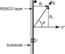
Figure 1. Schematic showing magnetic field angle, θ, relative to the REBCO wire cross-section, defining the radial field component, Br, and the axial field component, Bz. The plane of the field variation is maintained perpendicular to the current flow direction, I (maximum Lorentz force geometry). A dot is used to uniquely indicate the orientation of the wire with regard to its inherent asymmetry; θ is positive for rotations of the field towards the dot.
Download figure:
Standard image High-resolution image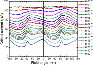
Figure 2. Measured Ic (B, θ) dependence at 77 K of the 4 mm wide SuperPower SCS4050-AP wire used for the end windings of the hybrid coil assembly. This data was previously presented in [13]. The asymmetry in Ic to either side of ±90° is apparent, and is particularly strong at fields between 0.05 T and 0.20 T.
Download figure:
Standard image High-resolution imageFurthermore, intensive AC loss analysis of HTS coils has been carried out both experimentally and numerically [14–20]. However, there has been no report to date on the influence of asymmetric wire critical current on coil AC loss. In this work, we explore the influence of wire Ic asymmetry on overall coil Ic as well as on the AC loss of hybrid coil assemblies [21–23].
The concept of hybrid coil assemblies arises due to the fact that conductors situated in different parts of a coil winding experience different magnetic field strengths and orientations, and therefore that using different conductors in the central and end parts of the coil can improve both the Ic and the AC loss of the overall coil [22] while simultaneously minimizing cost. Here, we go one step beyond this and consider improvements in performance that can be achieved simply by being aware of the relative orientations of the different windings as they are put together to form the coil assembly.
The question we seek to answer is: if hybrid coil assemblies are formed using the same coils but simply arranging the wire orientation in the different windings to take advantage of the inherent wire asymmetry, can we get not only increased Ic but also lowered AC loss in the overall assemblies?
2. Experimental methods
The coil assemblies studied comprise two end windings and one central winding as shown in figure 3. The end windings consist of one double pancake each while the central winding is formed from a stack of four double pancakes. The different windings are all wound with SuperPower SCS4050 AP wires with higher performance wire being selected for the end windings (104 A nominal 77 K self-field Ic compared to 86 A for the central windings) [24]. This highlights the benefit of hybrid coil assemblies in that maximal performance can be achieved using a cheaper wire for the bulk of the windings. Figure 4 shows the completed windings prior to assembly. HTS-110 Limited wound the coils with the superconductor layer facing the outside and maintaining the same wire orientation for each coil in the stack.

Figure 3. Schematic of the hybrid coil assembly studied in this work, and the magnetic field profile generated when it is energized. The assembly comprises a double pancake for each of the end windings and a stack of four double pancakes for the central winding.
Download figure:
Standard image High-resolution image
Figure 4. The central winding and end windings before assembly, also showing the BSCCO current leads used to supply current to the coil assembly.
Download figure:
Standard image High-resolution imageThree arrangements of the same set of coil windings have been constructed for this work: one arrangement is the same assembly featured in our previous work [23], where the detailed coil dimensions and construction method can be found. This we call the no-flipped assembly. In the second arrangement, the top end winding was turned upside-down leaving the central winding and the bottom end winding unchanged. This we call the one-flipped assembly. In the third arrangement, also the bottom end winding was turned upside-down to yield a configuration with both end windings reversed with respect to the original. This we call the both-flipped assembly.
Both the overall coil Ic and the AC loss of all three assemblies were measured and compared. The measurement method is described in detail in our previous work [22] and here we just recap the main points of the method. The coil assemblies were put in a foam-insulated liquid nitrogen dewar, the temperature of which is variable from 77 K to 65 K by reducing the pressure by pumping. Voltage taps were attached to the ends of the series windings for measuring both the Ic and the AC loss of the assemblies. Two Stanford Research Systems SR830 DSP Lock-in Amplifiers were used for AC loss data acquisition, one for registering the coil current and phase using a two-stage current transformer and the other for measuring voltage from the voltage taps. The Ic and AC loss measurements were carried out at both 77 K and 65 K.
3. Numerical methods
An axisymmetric 2D H-formulation finite element method simulation was carried out using COMSOL to calculate the expected AC loss of the coil assemblies [25]. Details of the simulation can be found in our previous work [26]. A combination of a structured mesh [27], edge elements [28], and a homogenization method [29] were used to reduce computing time. Figure 5 shows the structured mesh of the conductors forming the coil assemblies. Each pancake was divided into 40 elements along the axial direction and six sub-blocks in the radial direction.
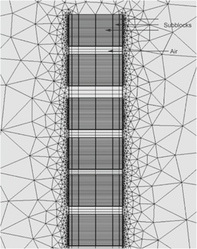
Figure 5. Structured mesh of the conductors forming the coil assemblies. A cross section of the top half of the conductor stack is shown. Each pancake coil is divided into 40 axial elements and six radial sub-blocks. Three axial air elements separate each pancake coil, and there is a larger air gap between the end winding and the central windings than between adjacent central windings.
Download figure:
Standard image High-resolution imageFor the central winding, the superconductor property is given as a non-linear E-J power law, E = Ec (J/Jc (B))n, where Jc (B) is the magnetic field-dependent critical current density, Ec = 10−4 V m−1, and n = 30. We adopted a modified Kim model [30] for the Jc (B) relationship incorporating its angular dependence [31]:

where B0 = 41 mT, k = 0.41 and a = 0.24 are fitting parameters obtained from the measured Ic(B) curves shown in figure 6 when the wire is exposed to a radial magnetic field, Br, or an axial magnetic field, Bz. Ic (B) is the integration of Jc (B) over the cross-section of the superconductor. For the end windings, the measured asymmetric Ic (B, θ) dependence of the 104 A 4 mm wide SuperPower SCS4050 AP wire at 77 K (figure 2) was used.
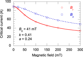
Figure 6. Measured Ic(B) curves (data points) and fitting curves (lines) in radial and axial magnetic fields for the SuperPower SCS4050-AP wire used to form the central winding of the hybrid coil assemblies.
Download figure:
Standard image High-resolution imageFigure 7 shows a cross-section of the right side of the hybrid coil assembly superimposed on the field distribution resulting when the coil is energised with 40 A AC current. As shown on the figure, the inner and outer turns of the end windings are exposed to strongly differently oriented magnetic fields. We consider an inner turn in the top end winding as marked in red on the figure. If we define the upper edge of the turn as a reference for the wire orientation, then the field angle relative to the wire is α as shown on the right side of the figure. However, if we flip the upper end winding then the field angle will become −α for the coil turn in the same position because the wire reference edge is now the lower edge of the winding as illustrated on the far right of the figure. In the same way, we can consider the effect of flipping the end coils on the field orientations relative to the wire for each of the inner and outer turns in the top and bottom end windings, with the results shown on the figure. The resulting field orientations for the inner turn are α, −α, 180° −α, and − (180° − α) and for the outer turn −β, β, − (180° − β), and 180° −β.

Figure 7. Cross-section of the right side of the hybrid coil assembly superimposed on the field distribution resulting when the coil is energised. Turns marked in red and blue represent inner and outer turns of the top and bottom end windings at which indicative field directions are shown. The field angles relative to the wire for each coil orientation are shown on the right side.
Download figure:
Standard image High-resolution imageTherefore, with fixed central windings, there are four possible values for the Ic (B, θ) properties of the end windings related to their wire orientation: upper reference edge for the top end winding and upper reference edge for the bottom end winding (denoted UU), upper edge for the top end winding and lower edge for the bottom end winding (UL), lower edge for the top end winding and upper edge for the bottom end winding (LU), and lower edge for the top end winding and lower edge for the bottom end winding (LL).
If we assume α ≈ 60°, then −α ≈ −60°, 180°− α ≈ 120°, and −(180°−α) ≈ −120°. If we look at figure 2, we see that the Ic value at −60° is greater than that at 60°, and the Ic value at 120° is greater than that at −120°. This implies that the LU assembly is most desirable in respect of the inner turns for a higher overall assembly Ic value. On the other hand, if we assume β ≈ 30°, then − β ≈ − 30°, 180° −β ≈ −150°, and − (180° −β) ≈ −150°. Again referring to figure 2, the Ic value at −30° is greater than that at 30°, and the Ic value at 150° is greater than that at −150°. This implies that the UL assembly is most desirable in respect of the outer turns, which is the opposite of the above. Therefore, the final Ic value of the coil assemblies depends largely on the local magnetic field throughout the assembly, and numerical simulation taking into account the measured Ic (B, θ) is necessary to predict the overall Ic value of coil assemblies.
For both critical current and AC loss simulations, we used Jc (B, θ) values deduced from the measured Ic (B, θ) shown in figure 2, by generating a three column look-up table [Bradial, Baxial, Jc (Bradial, Baxial)], where Bradial and Baxial are the radial and axial components of the magnetic field, and using the direct interpolation method [32]. If the field angle is α, Bradial = Bcos(α) = Br and Baxial = Bsin(α) = Bz as shown in figure 1. The Bradial and Baxial components of the other field angles shown in figure 7 can be calculated in a similar way, resulting in the set of components shown in table 1 for the four different assemblies. AC loss values in the four different assemblies were calculated by using the different asymmetric Jc (Bradial, Baxial) values for the end windings in these four possible configurations.
Table 1. (Bradial, Baxial) components determined from the field angles in figure 7 for different coil arrangements.
| UU | UL | LU | LL | |
|---|---|---|---|---|
| Top end winding | (Br, Bz) | (Br, Bz) | (Br, −Bz) | (Br, − Bz) |
| Bottom end winding | (−Br, Bz) | (−Br, −Bz) | (−Br, Bz) | (−Br, −Bz) |
Assembly Ic (Ic,coil) values can be determined from the following equation [13],

where Eave is the average electrical field across the entire coil assembly cross section, S. Ic,coil was defined when Eave reaches 1 μVcm−1.
4. Experimental and numerical results and discussion
4.1. Ic measurement of coil assemblies
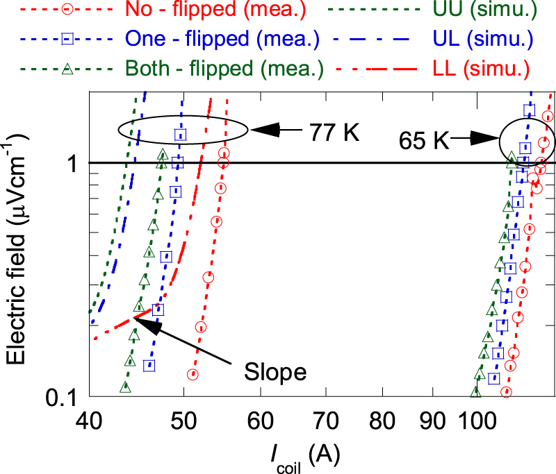
Figure 8 shows the E-I curves of the three coil arrangements measured at 77 K and 65 K, after subtracting the voltage contribution resulting from the contact resistance between the double pancakes [22]. In this figure, the calculated E-I curves in the UU, UL, and LL assemblies are plotted together. The UU, UL, and LL assemblies correspond to the no-flipped, one-flipped, and both-flipped assemblies, as discussed later in section 4.2. Table 2 summarizes the different measured and calculated Ic,coil values, determined at E = 1 μVcm−1. At both temperatures, the Ic of the assemblies follows the trend of no-flipped > one-flipped > both-flipped. The measured Ic value of the no-flipped assembly is 16% higher than that of the both-flipped assembly at 77 K, and 7% higher at 65 K. The calculated Ic,coil values can successfully predict the same tendency as the measurement even though the agreement between the measured and simulated results is not perfect. It is worth noting that the calculated Eave values contain a linear component (slope) which we attribute to dynamic resistance which occurs when superconductors carry DC current under changing magnetic field [33]. Similar simulation results were observed in previous research [10]. The slope is related to the ramp rate, and a smaller ramp rate gives a gentler slope and hence smaller error for the Ic,coil calculation. The existence of the slope is one of the reasons for the disagreement between the measured and simulated results. The results reconfirm the fact that coil assembly Ic values can be increased or decreased simply depending on how the wire is oriented in the coil windings.
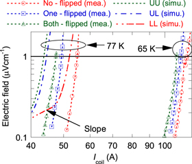
Figure 8. Comparison of the measured and calculated E-I curves of the various coil arrangements at 77 K and 65 K.
Download figure:
Standard image High-resolution imageTable 2. Measured and calculated coil assembly Ic values at 77 K and 65 K.
| Assembly geometry | Measured coil Ic at 77 K (A) | Calculated coil Ic at 77 K (A) | Measured coil Ic at 65 K (A) |
|---|---|---|---|
| No-flipped | 54.9 | 52.0 | 116.3 |
| One-flipped | 49.3 | 44.5 | 111.5 |
| Both-flipped | 47.5 | 43.7 | 108.4 |
4.2. AC loss measurement of coil assemblies
Figure 9 shows the measured AC loss values in the no-flipped assembly at 13.96 Hz, 19.80 Hz, and 26.62 Hz at 77 K and 65 K plotted as a function of the amplitude of the coil current, Icoil. The AC loss values obtained at different frequencies agree at both temperatures. This implies the AC loss in the assembly is hysteretic [22, 34]. Similar results (not shown) were obtained for the other two assemblies.
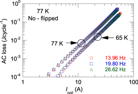
Figure 9. Measured AC loss at different frequencies in the no-flipped assembly at 77 K and 65 K.
Download figure:
Standard image High-resolution imageFigure 10 compares the normalised AC loss values in the three assemblies plotted as a function of Icoil normalised by the measured coil Ic values. As shown in the figure, the normalised AC loss values at the two temperatures are in very good agreement for all assemblies. This same result was observed in our previous works [21, 22]. The results re-confirm that AC loss in the coil assemblies can be scaled with the coil Ic values.

Figure 10. Comparison of normalised AC loss values in the three coil assemblies at 77 K and 65 K: (a) the no-flipped assembly, (b) the one-flipped assembly, and (c) the both-flipped assembly.
Download figure:
Standard image High-resolution imageFigure 11 compares the measured AC loss values in the three different coil assemblies. The figures are plotted on a linear scale to observe the differences more clearly. At both temperatures, the AC loss of the assemblies follows the trend of no-flipped < one-flipped < both-flipped. This trend is opposite to the Ic result, i.e. the larger the Ic, the smaller the AC loss, consistent with the observation in our previous works [21, 22]. In other words, AC loss in hybrid coil assemblies can be reduced by increasing the assembly Ic, as the AC loss in coil assemblies wound with REBCO wire increases with the 3rd to 4th power of It/Ic. The AC loss of the no-flipped assembly at 77 K is 13% lower than that of the both-flipped assembly at 40 A. The difference in the AC loss values of the assemblies at 65 K is even larger. This is the first demonstration that shows if we wind hybrid coils smartly using the same materials and the same design, we can not only improve Ic but also reduce the AC loss of the assembly.
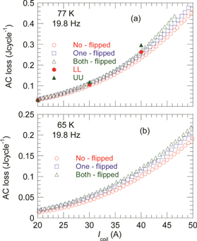
Figure 11. Comparison of measured AC loss in the three different coil assemblies at 19.80 Hz and (a) 77 K, (b) 65 K. In (a), simulation results for the LL and UU assemblies at 20 A, 30 A, and 40 A are marked.
Download figure:
Standard image High-resolution imageTable 3 summarises the simulation results for the four possible coil arrangements at four different coil currents. Mimicking the experimental results, there is a systematic difference in the AC loss values for the different coil assemblies. For a given coil current, the AC loss in the LL assembly is the lowest and that in the UU assembly is the highest. The LU assembly and the UL assembly have approximately the same AC loss, between that of the LL and UU assemblies. As the coil current increases, the difference in AC loss also increases. The decrease in AC loss at 40 A is 11% which is close to the difference in the measured values for the no-flipped and both-flipped coil assemblies.
Table 3. Simulated AC loss results for the four possible coil arrangements at four different currents, at 77 K. The reduction in AC loss of the LL configuration compared to the UU configuration is also shown.
| AC loss (J/cycle) | |||||
|---|---|---|---|---|---|
| Coil current (A) | UU | UL | LU | LL | (QUU− QLL)/QUU (%) |
| 10.0 | 3.74e-3 | 3.63e-3 | 3.64e-3 | 3.53e-3 | 6 |
| 20.0 | 3.21e-2 | 3.08e-2 | 3.09e-2 | 2.96e-2 | 8 |
| 30.0 | 1.17e-1 | 1.11e-1 | 1.11e-1 | 1.05e-1 | 10 |
| 40.0 | 2.96e-1 | 2.80e-1 | 2.80e-1 | 2.63e-1 | 11 |
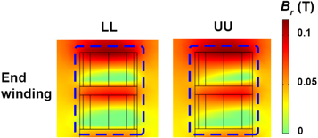
Figure 12 shows the radial magnetic field distribution in the end windings of the LL and UU assemblies (see enclosed with blue dashed lines) for a coil current of 40 A. Although the field distribution is broadly similar in the two arrangements, there is a clear difference between the two differently arranged end windings on the inner (left) side. The region of the end windings with high radial magnetic field component (red colour) is much greater in extent in the UU assembly than in the LL assembly. Because AC loss in coated conductors is determined by the perpendicular (radial) magnetic field component, this region is decisive in determining the overall AC loss of the coil [35]. This explains why the AC loss in the LL assembly is lower than that in the UU assembly.
Figure 12. Distribution of the radial magnetic field Br in the end windings (see enclosed with blue dashed lines) of the best (LL) and worst (UU) assemblies for a coil current of 40 A. There is a significant difference between the radial magnetic field components in the inner (left side) end windings of the two assemblies.
Download figure:
Standard image High-resolution image
A single wire orientation was maintained during winding of all the coils. Therefore, the no-flipped assembly which has the same wire orientation in both end windings must be either the UU assembly or the LL assembly. Because the no-flipped assembly has the smallest measured AC loss and the LL assembly has the smallest calculated AC loss, we can easily conclude that the no-flipped assembly is the LL assembly. Then we can identify the both-flipped assembly as the UU assembly and note that its AC loss values are the largest. Finally, we can conclude that the one-flipped assembly is the UL assembly which has AC loss values between the UU and LL assemblies. In figure 11(a), the AC loss simulation results for the LL and UU assemblies taken from table 3 are compared with the experimental results. A reasonable agreement was obtained between the simulated and measured values. Therefore, the simulation result replicates the experimental result. E.g. the difference between the measured and simulated results at Icoil = 30 A for the LL is 2% and 11% respectively. The radial field distributions in figure 12 also explain why the no-flipped (LL) assembly has greater coil Ic than the both-flipped (UU) assembly, due to the lower radial (out-of-plane) fields present.
5. Conclusion
In this work, we have built three hybrid coil assemblies which have a common central winding and a different geometrical arrangement of the same end windings. The critical currents and AC losses of the assemblies were measured at both 77 K and 65 K. A 2D finite element method AC loss simulation of the assemblies at 77 K was carried out using H-formulation to provide insight into the experimental results.
We observed a notable difference in critical current of the different assemblies, even though the windings used the same materials and share the same design. At both 77 K and 65 K, the Ic of the assemblies followed the trend no-flipped > one-flipped > both-flipped. The measured Ic value of the no-flipped configuration was as much as 16% higher than the other configurations at 77 K. The results reconfirm the fact that coil assembly Ic values can be increased or decreased significantly depending on how the wires are oriented in the coil windings.
We also observed a substantial difference in AC loss values between the three coil assemblies. At both temperatures, the AC loss values of the assemblies followed the opposite trend to the Ic values, with higher Ic corresponding to lower AC loss. The reduction in the measured AC loss of the no-flipped configuration compared to the both-flipped configuration at 40 A, 77 K was 13%. According to the simulation, the variation in both AC loss and Ic in the different assemblies is due to the difference in the radial magnetic field in the inner part of the end windings.
This is the first demonstration that shows if we wind hybrid coil assemblies smartly even using the same materials and the same design, we can not only improve the overall critical current of the assembly but also reduce its AC loss.
Acknowledgments
This work was supported by the New Zealand Ministry of Business, Innovation and Employment Contract No. RTVU1707. The research was partially supported by the Japan Student Services Organization who provided a scholarship for N E to visit Victoria University of Wellington. Z J acknowledges the assistance of Gennady Sidorov in the development of the specialist cryostat used in this work.