


Abstract
Despite the importance of preserving contiguous tropical forest areas to maintain biodiversity and terrestrial carbon stocks, methodological challenges continue to hinder broad-scale analysis of threats to these forests. Emerging Hot Spot Analysis (EHSA) is a spatial-statistical method that conveys complex information about the temporal dynamics of deforestation across a range of moderate to coarse spatial scales. Using Global Forest Change (GFC) data as inputs, EHSA produces spatially comprehensive, gridded outputs that represent a standardized, reproduceable way to instantiate contiguous forest tracts as spatial objects. Doing so allows aggregation of other GFC-derived values and analysis of alternative geographic configurations besides sub-national jurisdictions or protected areas, which can limit observation of finer scale variations. This paper illustrates the method's utility to comprehensively characterize the magnitude and temporality of pressures facing the Selva Maya, a transboundary forest region with extensive areas under conservation that covers portions of Mexico, Guatemala, and Belize.
Export citation and abstract BibTeX RIS
1. Introduction
Deforestation threatens terrestrial carbon stocks, habitat, and biodiversity and is a recognized consequence of new and traditional land uses and their co-constituted livelihoods (Ellis et al 2021). Some of these activities, such as monoculture agriculture, may drive extensive loss of forest that is effectively permanent, with a low likelihood for regrowth in the near future, and thus high likelihood of permanent biodiversity loss (Rudel et al 2009, Dudley & Alexander, 2017). Even other activities such as logging and infrastructure development, where practices may be purposefully managed to limit the direct impacts on forest area loss, can still affect contiguity and patch size of forest and increase access to land that can open up new agricultural frontiers (Norris, 2008, Socolar et al 2019).
Globally, there are a limited number of large, contiguous tracts of tropical forest where challenges to access have prevented severe loss of biodiversity and biomass, and thus these are important targets of forest protection efforts (Senior et al 2019, Hansen et al 2020). At the same time, given increasing fragmentation, discrete forest tracts located in proximity to one another and arrayed in a way that their benefits are manifest at broader scales as a corridor still contribute to conservation goals. These forests are large enough to straddle the borders of multiple countries, bringing them under a heterogenous range of governments, politics, and governance regimes that are often assessed independently of one another by analyses of forest loss.
Spatial and temporal scale are both fundamental factors for measuring and analyzing forest trends; however, assessing and visualizing both in tandem has proven complicated. To understand ongoing and accelerating threats to forests there is an urgent need to analyze forest change and to communicate findings at the regional scale (106–107 m square), but many of the methods currently deployed to accurately detect and measure deforestation rely on observations made at the much finer scale of 101–102 m. And beyond analysis there are challenges of visualization: at regional scales the effective spatial resolution of data is determined by screen resolution and it becomes difficult to identify finer-scale patterns (figure 1).
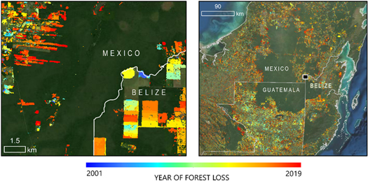
Figure 1. Multichromatic color schemes depicting year of forest loss can highlight the initiation or expansion of deforestation at fine spatial scales (left), but are not as easily interpretable at regional extents (right).
Download figure:
Standard image High-resolution imageSatellite data pre-processing and distribution allow for an abundance of moderate spatial resolution data, sometimes up to dozens of images per year for a given location. The annually updated, Landsat-based Global Forest Change (GFC) data (Hansen et al 2013) provide an input for standardized analysis of deforestation globally. Many regional-scale GIS analyses of deforestation convey the total amount of forest lost over a specific time period, and may, depending on the focus of the study, designate important proximate drivers of change during that time (Curtis et al 2018). Measurements of forest loss can be summed over broad areas, but this can risk eliding the interacting social, economic, and political processes at work in forest loss. Explaining trends in forest loss at regional scales would benefit from tools and methodologies that can capture within-region spatio-temporal pattern differences (Andrienko et al 2010, Goldman et al 2020). One such spatial statistical tool is Emerging Hot Spot Analysis (EHSA). This tool can analyze a dataset of events, outputting a grid of cells that are categorized using a schema that describes the abundance of features at, and around, a location over time. Together these convey the spatio-temporal patterns of change, and the method is well suited to study deforestation (cf Harris et al 2017).
This paper uses EHSA within ArcGIS Pro as the basis to describe spatial and temporal variation of deforestation at the meso-scale, between that of the cell resolution of inputs derived from remotely sensed data and the zones over which summary statistics are typically tabulated, such as national boundaries. The paper then shows the utility of such descriptive layers for understanding processes of change in the Selva Maya forest that covers portions of Guatemala, Mexico, and Belize. We argue that centering statistical analysis on the forests themselves, rather than administrative areas, greatly increases the depth of understanding that results can provide to conservation, climate change, or development planning. Indicating where losses have been greatest and where are they accelerating is vital for directing interventions in vulnerable landscapes, influencing the policies and structures through which those interventions will be governed.
2. Methods
2.1. Study area
The Selva Maya is the northernmost part of the Mesoamerican Biological Corridor (MBC), an extensive chain of forest tracts designated as a policy target for species and habitat conservation in the mid-1990 s (Herrera 2003, Holland 2012). Protected areas are an important component of MBC, but from its start this initiative also aimed to provide connectivity between protected areas, including across borders: only about half of the MBC's area is under official protection. The MBC stretches from southern Mexico to Panama, and since its inception has been contentious due to issues of scale and intervention, and the varying degree of local communities' involvement with habitat protection efforts brought on as part of a regional integration initiative.
Recent deforestation rates affecting Selva Maya have been sufficiently high for the World Wildlife Fund for Nature to label it as one of twenty-four global deforestation fronts (WWF 2021). Two areas are of special concern: frontier deforestation around the periphery of Selva Maya's largest intact forest tracts, and the corridor zones between these larger tracts.
2.2. Emerging hot spot analysis
EHSA is a process that implements the Getis-Ord Gi* spatial statistic, identifying where values of a variable at a location—and in the neighborhood around it—are significantly higher or lower when compared to the distribution of values across the entire input dataset ('hot spots' and 'cold spots', respectively). These patterns can be identified repeatedly for each time-step in the duration of study: EHSA introduces a temporal dimension to this analysis, so that the set of 'neighboring' values used in the determination of a hot/cold spot is defined in both space and time. The analyst can vary model parameters to specify the spatial neighborhood that will influence the spatial scale of the output, and select the distribution of input values from which determinations of significance are drawn.
EHSA uses a structure called a space-time cube, in which sums of values or points counts are calculated for 'bins' in two spatial and one temporal dimensions. The output of EHSA is a two-dimensional grid in which cells are categorized on the basis of temporal patterns of clustering. In this output, the modifiers 'new,' 'consecutive,' 'persistent,' 'intensifying,' 'sporadic,' 'diminishing,' and 'historical' describe the timing, trend, and temporal consistency of high or low amounts of deforestation at each location (table 1, see Esri 2021). The categorization makes use of four factors to characterize each grid cell: whether the final time step is a hot spot, whether greater than 90% of time steps are hot spots, whether there is significant change over time in how hot a hot spot is, and whether a cold spot was ever observed in any time step. Note the logic is symmetrical for cold spots, and that not all factors are relevant for each category definition (table 1).
Table 1. Definitions of categories used in EHSA outputs, with respect to hot spots.
| Hot spot category type | Is the final time step hot? | Have >90% of time steps been hot? | Has there been significant change in how hot? | Has location ever been a cold spot? |
|---|---|---|---|---|
| New | Yes | No | n/a | n/a |
| Consecutive | Yes | No | n/a | n/a |
| Intensifying | Yes | Yes | Yes, increasing | n/a |
| Persistent | n/a | Yes | No | n/a |
| Diminishing | Yes | Yes | Yes, decreasing | n/a |
| Sporadic | n/a | No | n/a | No |
| Oscillating | Yes | No | n/a | Yes |
| Historical | No | Yes | n/a | n/a |
The resulting abundance of categories, up to 17, has led many users to remove all cold-spot categories and merge hot-spot categories (e.g., Harris et al 2017, Hettler et al 2018, Goldman et al 2020). In this paper we similarly merge hot spots that are sporadic and oscillating, those that are new and increasing, and those that are persistent and consecutive to reduce the number of categories used while grouping on the basis of consistency, trend, and magnitude. While we also do not make use of most cold spot categories because the process of forest loss is asymmetric with a zero-lower bound, we do include diminishing cold spots, as these mark the location where very recent upticks in forest loss have been recorded with the potential for more severe future increases.
2.3. Data processing
We downloaded gridded 30 m spatial resolution Global Forest Change (GFC) v1.7 data (Hansen et al 2013) for the rectangular area ((−92.0, 21.5) to (−86.5, 16.0)) that covers Belize and portions of Mexico and Guatemala from Google Earth Engine. This analysis used three bands from this dataset: treecover2000, describing percent canopy closure in year 2000; lossyear, describing the year of forest loss for each year 2001 to 2019; and gain, describing the gain of forest occurring sometime during the period 2000–2012.
Processing of data for EHSA input was as described in Harris et al (2017); see also Goldman et al (2020). A NETCDF space-time cube was constructed by aggregating these lossyear points and input to EHSA. These three dimensional arrays have a default spatial extent that matches that of the input points and user-determined bin dimensions. A 5 km grid spatial resolution, and a 15 km spatial neighborhood distance were used, along with a 1-year time step that matches the temporal precision of the GFC lossyear data.
One simple benefit of EHSA for deforestation analysis relates to the aggregated grid on which spatial statistical results are displayed. This geographical layer provides flexibility to summarize results at scales where existing administrative jurisdictions are inadequate for capturing broader forest dynamics, and this works as well for the summarization of other data from the GFC product that complements lossyear. Here, a binary map of forest in year 2000 was produced by thresholding treecover2000 such that all pixels with a value greater than 30 were designated forest. This 30% threshold is similar to the value of 25% used in Hansen et al (2010) and was chosen after a comparison of output binary forest maps to high resolution images of forest in the study area indicated that this higher value yielded greater accuracy. A binary map approximating forest in year 2020 was produced by subtracting any pixel of observed forest loss from the binary map of forest in year 2000. These values were aggregated to the features of the same grid used in EHSA analysis, and using the values of forest in 2000 and 2020 a portion-forest-loss was derived for each cell. Finally, the ratio of total observed forest gains 2000–2012 and the amount of deforestation 2000–2012 was calculated for each cell as a proxy measure estimating net forest turnover.
3. Results
Measures of forest abundance and fractional loss during the period 2000–2020 (figure 2), calculated at 5 km spatial resolution, provide a basis for understanding regional change that can be complemented by results of EHSA. These first-order change maps show the areas of greatest gross forest loss in the south of the region, as well as in pockets in the east and west. A comparison of the 2000 and 2020 forest maps shows that these losses result in the fragmentation of what had been a large, contiguous expanse of forest. By 2020 there were fewer discrete forest tracts. One such large tract falls within the Calakmul Biosphere Reserve in Mexico, portions of the Maya Biosphere Reserve (MBR) in Guatemala, and areas of mixed protection status in Northern Belize. Another covers much of southern Belize.
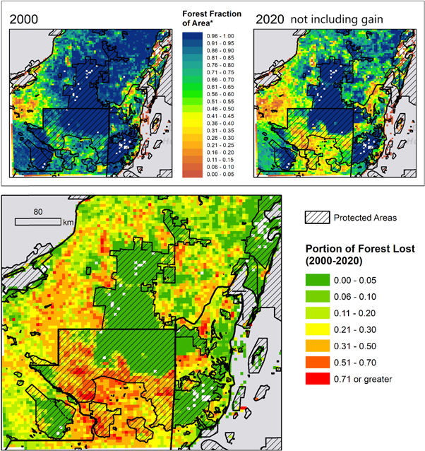
Figure 2. Above: Forest in 2000, and an estimate of minimum potential Forest extent in 2020 that accounts for all observed losses of forest but not gains. Below: Loss as a % of forest in 2000.
Download figure:
Standard image High-resolution imageProtected Area boundaries closely trace the deforestation frontiers in Mexico and in Belize, but in Guatemala there is a wide range of outcomes within protected areas: substantial areas where very little loss occurred as well as areas with very rates of deforestation > 70%. In Mexico, rates of loss were generally higher to the west of Selva Maya than to the east, and in central Belize there is a noticeable spatial gradient of loss within the corridor between the two large forest tracts, with loss rates >70% in the north and rates < 30% to the south.
While other spatial statistical analyses would also yield standardized measurements of how spatially concentrated forest loss was during the time period of interest, EHSA also allows us to disaggregate this trend temporally and highlight variability in timing, speed, and consistency of deforestation (figure 3).
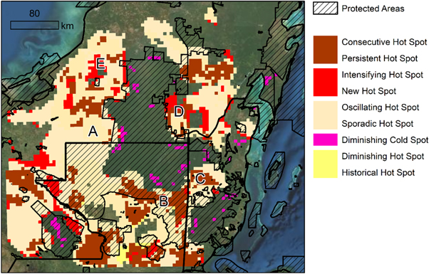
Figure 3. EHSA results for Selva Maya.
Download figure:
Standard image High-resolution imageThe agricultural frontier hot spots to the west of the Calakmul-MBR forest tract in Mexico and Guatemala (A) are largely categorized as Oscillating/Sporadic. Where these hot spots extend into proximal protected areas, New Hot Spots and Diminishing Cold Spots are visible.
The large deforestation frontier in northeast Guatemala (B) is primarily Consecutive/Persistent, signifying broad and robust land-cover change in these locations that has driven forest loss. Consecutive/Persistent hotspots linked to this frontier as it extends into central Belize (C). However, a greater portion of the Hot Spot cells covering the area between the Calakmul-MBR and southern Belize tracts of the Selva Maya are Oscillating/Sporadic, implying a less intense drive to deforest.
Areas to the east (D) and west (E) of the Calakmul-MBR tract in Mexico contain numerous and expanding Intensifying/New hot spots, and this can undermine the connectivity between the large portion of that tract that is under protection and smaller, nearby tracts that are not within a protected area.
One final variable that can aid in identification of the drivers of deforestation, with implications as to the severity and permanence of forest loss, is a ratio of the observed forest regrowth and gross deforestation during the period 2000–2012 (figure 4). This metric can serve as a proxy for rates of forest regrowth: high values indicate the local prevalence of shifting cultivation, speculative clearing, or clandestine air strips while lower values signal permanent, intensive agriculture or ranching. Figure 4 shows a clear divergence in values on either side of the Mexico-Guatemala border, with substantial areas in Mexico where the gains-to-losses ratio is between 0.25 and 0.75, in contrast to the much lower regrowth rates < 0.1 that are typical across much of northern Guatemala. Within the corridor area in central Belize between the Calakmul-MBR and southern Belize forest tracts there is a wide range in ratio values, from as low as 0.01 to as high as 0.8.
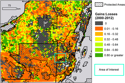
Figure 4. Ratio of forest gains to losses over the period 2000–2012. Extremely low values were observed in core forest areas, which had essentially no losses at all, and so these values are de-emphasized. Blue rectangle shows area between two largest forest tracts of Selva Maya for reference.
Download figure:
Standard image High-resolution image4. Discussion
EHSA can summarize complex temporal dynamics of forest cover change at the regional scales that can help assess conservation priorities. The large number of categories used in EHSA outputs can be unwieldy, but these categories correspond to important spatial-temporal textures for characterizing drivers of change, including shifting cultivation, monoculture conversion and pasture, or new infrastructure development. The meso-scale spatial resolution of EHSA outputs provides particular benefits for visualizing activities that entail a high gross amount of land change, such as shifting cultivation, by summarizing a high number of pixels that mark those change events. While this is true of the EHSA results generated in this paper using a grid resolution of 5 km and a spatial neighborhood of 15 km, a visual comparison of outputs using different values for these parameters (figure 5) indicates that the same patterns are evident with more or less spatial precision.

Figure 5. EHSA outputs generated using grid resolution/spatial neighborhood of (A) 2.5 km/7.5 km, (B) 5 km/15 km, and (C) 10 km/30 km.
Download figure:
Standard image High-resolution image
Such attention to the temporality of land change can be absent from other techniques of regional analysis that rely on differences observed over broad time intervals, and can complement analysis structured around discriminating the stressors facings forests and their levels of resilience (Saatchi et al 2021). The spatial variability evident in results can also highlight the distribution of risk as well as key areas at finer spatial scales where focused efforts can efficiently meet top-line conservation priorities. Localized patterns include isolated new fronts, marked by categories such as New Hot Spots or Diminished Cold Spots, where monitoring may be appropriate; kettling deforestation where the size of forest tracts has been diminished through the gradual encroachment of surrounding development, or rapid, bisecting incursions brought on by expansion of transportation infrastructure. Pronounced cross-border variation in the location of peripheral deforestation indicates the varying efficacy of legal forest protection efforts in Selva Maya: in Mexico and much of Belize, deforestation occurred up to but not beyond protected area borders, while in Guatemala this was not the case, and substantial permanent loss of forest occurred within certain protected area boundaries.
EHSA reveals that that pressures around Selva Maya in Guatemala and Belize have produced more temporally consistent forest loss, without substantial forest regrowth, than in Mexico. While the spatial concentration of hot spots generally aligns with the areas seen in figure 2 that have experienced the greatest magnitude of loss, the additional temporal information provides insight about drivers and ecological consequences. In Mexico these rates of loss and regrowth are associated with the traditional milpa shifting cultivation that is practiced there (Parsons et al 2011). There is a clear difference across the border with Guatemala, where regrowth rates were much lower, typically below a 0.1 portion of forest lost, suggesting widespread pasture conversion.
Within this area of greatest and most consistent forest loss, however, are locations where observed dynamics ran against that trend. A portion of the area in central Belize that is well positioned to serve as a corridor between the large, protected tracts of the Selva Maya saw less deforestation, more sporadic deforestation, and relatively high forest regrowth. We highlight this smaller area, roughly 105 m square, as a critical area in which to focus campaigns for reforestation or protection, even more so than in the large area surrounding it that has been labelled by the Worldwide Fund for Nature (WWF) as a deforestation front (WWF, 2021). While Guatemala saw high levels of consecutive/persistent and oscillating/sporadic hot spots, including in protected areas, the core non-deforested zone coincides with lands managed by community concessions, rather than state or private interests. This spatial analysis provides additional evidence as to the robustness of that conservation and land use model in the face of significant drivers of land use/cover change (Bebbington et al 2018, Stoian et al 2018, Devine et al 2020).
5. Conclusion
A spatial analysis focused on any of the individual countries that contain some portion of Selva Maya would fail to provide these insights as clearly, if at all. Even a comprehensive study of the region that relied on existing feature geometries such as provincial borders or protected areas would also fail to describe important patterns of deforestation, particularly the variation in efficacy among protected areas and across patches. In contrast, the gridded output of EHSA provided a standardized way to aggregate values across border regions that pointed to specific priority conservation areas and indicated contrasting enforcement of law and policy within administrative areas. As land change proceeds along many frontiers and effects of climate change emerge, EHSA can be a particularly useful across regions where existing geographies may be heterogeneous such as border regions—where institutions, governance regimes, and implementation of conversation policy may sharply diverge.
Acknowledgments
This work was supported by the National Socio-Environmental Synthesis Center under funding received from the National Science Foundation DBI-1639145, and NASA (80NSSC21K1431). We would like to acknowledge the two anonymous reviewers who provided feedback on our submitted manuscript.
Data availability statement
The data that support the findings of this study are openly available at the following URL/DOI: https://doi.org/http://earthenginepartners.appspot.com/science-2013-global-forest.
Conflict of interest statement
The authors declare no conflicts of interest.