

Abstract
Greenhouse gas (GHG) emissions from reservoirs have most often been evaluated on a global extent through areal scaling or linear-regression models. These models typically rely on a limited number of characteristics such as age, size, and average temperature to estimate per reservoir or areal flux. Such approaches may not be sufficient for describing conditions at all types of reservoirs. Emissions from hydropower reservoirs have received increasing attention as industry and policy makers seek to better understand the role of hydropower in sustainable energy solutions. In the United States (US), hydropower reservoirs span a wide range of climate regions and have diverse design and operational characteristics compared to those most heavily represented in model literature (i.e., large, tropical reservoirs). It is not clear whether estimates based on measurements and modeling of other subsets of reservoirs describe the diverse types of hydropower reservoirs in the US. We applied the Greenhouse Gas from Reservoirs (G‐res) emissions model to 28 hydropower reservoirs located in a variety of ecological, hydrological, and climate settings that represent the range of sizes and types of facilities within the US hydropower fleet. The dominant pathways for resulting GHG emissions estimates in the case-study reservoirs were diffusion of carbon dioxide, followed by methane ebullition. Among these case-study reservoirs, total post-impoundment areal flux of carbon ranges from 84 to 767 mgCm−2d−1, which is less variable than what has been reported through measurements at other US and global reservoirs. The net GHG reservoir footprint was less variable and towards the lower end of the range observed from modeling larger global reservoirs, with a range of 138 to 1,052 g CO2 eq m−2 y−1, while the global study reported a range of 115 to 145,472 g CO2 eq m−2 y−1. High variation in emissions normalized with respect to area and generation highlights the need to be cautious when using area or generation in predicting or communicating emissions footprints for reservoirs relative to those of other energy sources, especially given that many of the hydropower reservoirs in the US serve multiple purposes beyond power generation.
Export citation and abstract BibTeX RIS

Original content from this work may be used under the terms of the Creative Commons Attribution 4.0 licence. Any further distribution of this work must maintain attribution to the author(s) and the title of the work, journal citation and DOI.
1. Introduction
Hydropower is a critical part of the global energy system, generating over 4,370 TWh of renewable energy in 2020 (IHA 2021). In the US, annual generation is roughly 274 TWh, representing 6%–7% of all electricity generated, and 38% of the electricity from US renewables (Uria-Martinez et al 2021). Emissions from hydropower reservoirs have received increasing attention as industry and policy makers seek to better understand the role of hydropower in sustainable energy solutions (O'connor et al 2016). Hydropower reservoirs, as well as non-hydropower reservoirs and lakes, can be hotspots for carbon burial (Mendonça et al 2017) and greenhouse gas (GHG) production and emissions (Bastviken et al 2011, Rosentreter et al 2021) due to physical and biogeochemical processes occurring in these aquatic ecosystems. Carbon dioxide (CO2) and methane (CH4) are the two main GHGs of interest at reservoirs. CO2 is produced via multiple processes, including the decomposition of organic matter, whereas CH4 is formed through the microbially mediated biogeochemical process of methanogenesis. Both gases are emitted from a reservoir through a variety of pathways including diffusion, ebullition (or bubbling), and degassing from water that passes through turbines or other outlet structures, though CH4 ebullition and degassing are rarely measured or modelled.
Understanding GHG emissions in individual reservoirs is a significant scientific challenge. Recent studies highlight challenges involved in carbon and GHG accounting at reservoirs (Prairie et al 2018), and particularly at hydropower reservoirs (Jager et al 2022). These challenges include variability in processes and pathways for GHG emissions which can change over space and time. Additionally, many factors are highly dependent on multiple biogeochemical processes in the reservoir, and emissions unrelated to the impoundment or operation of the reservoir (i.e., anthropogenic processes adding carbon to the system) can be difficult to estimate, but are important to be accounted for (Lovelock et al 2019).
One major obstacle to accurate quantification of GHG emissions is the difficulty of capturing temporal variation (Demarty et al 2011, Beaulieu et al 2014) and spatial heterogeneity both within (Beaulieu, McManus and Nietch 2016) and across water bodies (Deemer et al 2016, DelSontro, Beaulieu and Downing 2018). Synoptic sampling can result in underestimation, not accounting for variability in CH4 ebullition can result in underestimation total emissions by 50% (Deemer et al 2016) failure to capture extreme values (Prairie et al 2021). Despite inherent limitations of empirical measurements, they have often been used to estimate GHG emissions for other reservoirs by assuming fluxes scale solely based on area (Ehhalt 1974, St. Louis et al 2000, Cole et al 2007, Tranvik et al 2009, Rosentreter et al 2021). Some recent studies have extrapolated point measurements to reservoirs based on relationships with covariates such as productivity and lake size (DelSontro, Beaulieu and Downing 2018). Alternatively, regression techniques for predicting emissions have used reservoir-specific characteristics such as reservoir morphology, catchment land use (Beaulieu et al 2020), reservoir age (Barros et al 2011), and temperature (Scherer and Pfister 2016). However, these models are often limited to characteristics that are readily available from dam or reservoir inventories and may not represent many of the complexities of physical and biogeochemical processes contributing to GHG production and emission. Some relationships observed in smaller datasets have not persisted when more data were collected and analyzed. For example, as the sample of 85 reservoirs from Barros et al (2011) was expanded to 267 reservoirs, mean reservoir depth was no longer a strong predictor of CH4 flux (Deemer et al 2016). Beaulieu et al (2020) highlight that expanded sampling is needed to validate larger-scale extrapolation of these types of models to unsampled reservoirs.
On the other hand, physical models such as CE-QUAL-W2 (Wells 2021) and LAKE2.0 (Stepanenko et al 2016) represent hydrodynamic and biogeochemical processes well and have been used to model reservoir GHG emissions (Berger et al 2014, Guseva et al 2020), but have their own drawbacks. These include data-intensive input requirements (e.g., detailed bathymetry, physicochemical characteristics of the water column and sediments) and simplified representations of lake dynamics (e.g., only simulating 1 or 2 dimensions). This is particularly limiting when assessing emissions across bodies of water that are remote, incompletely mapped, or irregularly sampled and therefore cannot be properly calibrated or validated with physical models. Further, incomplete representation of processes by widely used lake and reservoir models necessitates coupling/coordination of different models (e.g., degassing is often not included in common lake or reservoir models).
Large-scale applications of models and aerial scaling of measurements to national or global estimates have resulted in different estimates for total flux and have been used to describe general patterns in flux and emissions across different pathways. Because of the diversity of types of hydropower reservoirs (sizes, operations, condition, watershed land use and hydroclimate) in the US, it is unclear if these coarse estimates and patterns in pathways describe the range of conditions that are observed in the US hydropower fleet.
In this study, we applied the Greenhouse Gas from Reservoirs (G‐res) tool (Prairie et al 2021), which estimates pathway-specific fluxes of CO2 (diffusive) and CH4 (diffusive, ebullitive, and degassing) at the reservoir level, to a diverse collection of 28 US hydropower reservoirs. The web-based G-res tool is based on a set of equations derived from an inventory of reservoir emission measurements. In addition to the more explicit representation of different pathways than what has typically been modelled in the past, the models in G-res also incorporate a broader suite of explanatory variables to describe catchment and reservoir characteristics relevant to the production and emission of GHGs. G-res is used to estimate per-reservoir and areal flux of CO2 and CH4. First, we evaluated key geomorphological and water quality characteristics of these 28 reservoirs to describe how this sample of reservoirs fits within the broader context of the larger US hydropower fleet and other reservoirs assessed in global inventories of GHG gases. Next, we evaluated modelled GHG emissions by pathway for the selected reservoirs, and compared these to empirical measurements and global G-res model estimates. This analysis highlighted which emission pathways were most dominant and described the range of GHG fluxes across a range of hydropower systems. Overall, our modelling analysis of US hydropower reservoirs results in a detailed understanding of the characteristics and conditions present at these reservoirs that drive GHG emissions. This information provides valuable insight to those who manage these systems and improves our understanding of the contribution of US hydropower reservoirs to global GHG and carbon accounting.
2. Data and methods
2.1. Site selection
Our first goal was to identify a representative set of reservoirs spanning the range of environments, locations, and types of conventional hydropower systems in the conterminous US (CONUS). We focused on reservoirs that were not immediately downstream of other reservoirs (i.e., cascading systems), though we did not strictly limit selection to headwater dams, since these are a relatively small proportion of hydropower facilities. Cascading systems were not included because the G-res model does not explicitly account for reductions or inputs to GHG emission processes that might be occurring in upstream reservoirs (Prairie et al 2017). From this set, we chose reservoirs from different ecoregions, prioritizing those with documented GHG and water quality measurements.
Unique hydropower reservoirs with operational power plants and inventoried reservoirs (n = 1,003) were identified from the Hydropower Infrastructure—LAkes, Reservoirs, RIvers database (HILARRI v1.1) (Hansen and Matson 2021) as candidates for model application. An additional 31 existing inventoried reservoirs in the pipeline for hydropower development (Johnson and Uria-Martinez 2021) were considered.
Candidate reservoirs from the initial screening were grouped by ecoregion, as defined by the US Environmental Protection Agency (EPA, Omernik and Griffith 2014). We assumed that the properties that distinguish these regions (i.e., type, quality, and quantity of environmental resources) are relevant for reservoir and catchment processes. We then targeted reservoirs included in one or more of the 2007, 2012, or 2017 EPA National Lake Assessments (NLA, USEPA 2016) or could be matched to the existing GHG measurement inventory by Deemer et al (2016). This was done to exploit existing information for G-res model inputs (e.g., the NLA includes reservoir characteristics and water quality information) and for comparison between modelled and measured results. At least one reservoir was selected from each ecoregion, most regions included at least two reservoirs and generally, ecoregions with higher abundances of hydropower reservoirs had proporitionally higher representation. A total of 28 reservoirs were selected based on the search criteria and referred to hereafter as 'case-study reservoirs' (figure 1). Six sites did not have water quality or GHG records from the NLA or GHG measurement inventory, but were still included for better representation across the geographic extent of the CONUS and the variety of ecoregions. Finally, sites were chosen to represent a spectrum of size (surface area and storage volume), age, and purposes. Characteristics of the case-study reservoirs were obtained from the dam and reservoir inventories. The process for selection and data sources is summarized in figure S1.

Figure 1. Locations of hydropower reservoirs and those selected as case-studies for G-res model application in this study. Identifiers shown for reservoirs correspond with those used in the National Inventory of Dams (USACE 2019).
Download figure:
Standard image High-resolution imageThe sample of case-study reservoirs ranged in surface area from 0.12 to 457 km2 (median = 19.7 km2) and in storage from 0.1 to 8,042 × 106 m3. The sample was skewed towards larger reservoirs, with 20 of the 28 total reservoirs exceeding the 75th percentile of all US hydropower dams linked to operational power plants and inventoried reservoirs for both surface area and storage (figures S2A, B). The range of age in case-study reservoirs was 28–110 years, spanning the 1st to the 75th percentile of US hydropower reservoirs (figure S2C). Case-study reservoirs were younger, with a median age of 63 years compared to 91 years for other US hydropower reservoirs. 86% of the case-study reservoirs serve more than one purpose besides hydropower compared to 72% of the US hydropower dams that also support other purposes (figure S2D).
The case-study reservoirs spanned a similar range in water quality characteristics as observed in the dataset of global hydropower reservoirs (Deemer et al 2016) and the dataset of US hydropower reservoirs in the NLA (figure S3). For chlorophyll-a (figure S3A), total phosphorus (figure S3B), and total nitrogen concentrations (figure S3C), the case-study reservoirs spanned from the lowest reported value in the NLA measurements through the 75th percentile, 88th percentile, and 93rd percentile, respectively. The three reservoirs with the lowest total phosphorus concentrations were included in the case-study, one of which also had the lowest chlorophyll-a concentration (French Meadows, CA00856). A different case-study reservoir had the lowest total nitrogen concentration (Upper Baker WA00173). As a result of this slight skew toward lower chlorophyll-a and nutrient concentrations, both the case-study reservoirs and US hydropower reservoirs underrepresent eutrophic systems compared to global reservoirs (figures S3D, E).
2.2. Inputs, assumptions, and application of the G-res model
G-res v.2.1 (Prairie et al 2021) was used to predict GHG emissions for the 28 case-study reservoirs. While detailed descriptions of the tool and validation of its underlying models are provided by the tool developers, we provide an overview of the key inputs and structure of the tool. Inputs to the G-res model consist of either characteristics of the catchment or the reservoir (physical and operational). The modelled system is not dynamic, so emissions are not simulated over a series of time steps. Instead, the model uses empirical models to calculate emissions on an annualized basis (e.g., g CO2 y−1). Inputs to the model are therefore static and assumed to be representative of reservoir conditions from impoundment to end-of-assumed-life (100 years). In many cases, inputs were derived from remotely sensed or modelled data (detailed in table 1) and required processing using GIS software or cloud-based processing in Google Earth Engine.
Table 1. Catchment and reservoir attributes and climate drivers used as inputs to the G-res model.
| Description (units) | Resolution | Source | Processing |
|---|---|---|---|
| Catchment/reservoir buffer parameters | |||
| Area (km2) | 10 m | USGS National Elevation Dataset | Used ArcGIS 10.7 to fill depressions, determine flow direction, accumulation, and delineate catchment boundary |
| Land cover | 30 m | 2016 National Land Cover Database (Dewitz 2019) | Calculated area as a percentage of catchment and reservoir buffer area |
| Soil carbon content (kgC m−2) | 250 m | SoilGrids Global Gridded Soil (Hengl et al 2017) Information | Calculated mean soil carbon content over the catchment and reservoir buffer area |
| Mean annual runoff in catchment (mm y−1) | 4 km | TerraClimate Monthly Water Balance for Global Terrestrial Surfaces (Abatzoglou et al 2018) | Aggregated the monthly mean runoff from 1990–2019 on an annual basis and calculated the annual average over the catchment area |
| Population in catchment | 1 km | 2020 Gridded Population of the World v4.11 (CIESIN Center for International Earth Science Information Network 2018) | Multiplied average density by the catchment area |
| Reservoir parameters | |||
| Average air temperature (°C) | 1 km | Daymet v4 Daily Surface Weather and Climatological Summaries | Calculated average monthly temperature over 1990–2019 from daily temperature over the reservoir area |
| Wind speed at 10 m (m s−1) | 4 km | Gridmet: University of Idaho Gridded Surface Meteorological Dataset (Abatzoglou 2013) | Calculated average annual wind speed over the reservoir area from 1990–2019 daily wind speed |
| Global Horizontal Radiation (kWh m−2 d−1) | 0.5 degree (∼55 km) | NASA Surface Meteorology and Solar Energy Release 6.0 (Stackhouse et al 2015) | Calculated average daily radiation over the reservoir area according to G-res technical guidance (Prairie et al 2017) for 1983–2005 based on latitude |
Specific inputs include water treatment (i.e., whether there were primary, secondary, or tertiary treatment facilities in the catchment), parameters describing the general morphology (volume, surface area, maximum depth) of the reservoir, and operations (intake depth and annual releases) at the dam. Several parameters (mean depth, thermocline depth, phosphorus loading, etc) were estimated using default G-res estimation methods; these default values were overridden if data were available through publicly available documents such as license documents, fishing depth reports, or published studies reporting water quality conditions (see Supplemental Data).
In this study, estimated emissions were based on reservoir characteristics only; life-cycle emissions attributed to materials and construction of the dam were not evaluated. Reservoir emissions were estimated for multiple pathways (diffusion, ebullition, and degassing for CH4 and diffusion for CO2) and reported as net emissions (i.e., pre-impoundment emissions and unrelated anthropogenic sources of emissions subtracted from post-impoundment emissions). Pre-impoundment emissions are based on factors related to land cover and soil types within a buffer around the perimeter of the reservoir. Conditions in the buffer were assumed to be representative of those that existed prior to impoundment of the river and filling of the reservoir. Emissions attributed to unrelated anthropogenic sources are associated with the input of phosphorus to the reservoir from human-related activities in the catchment (i.e., sewage and human-related land use) (Prairie et al 2017). For convenience in comparing emissions across the different pathways and GHGs, footprints were calculated as CO2 equivalents (CO2eq) using the default G-res 100-year horizon global warming potential factor (GWP100), where CH4 is multiplied by 34, the most conservative GWP100 reported by the IPCC Fifth Assessment Report (Myhre et al 2013). GHG footprints (overall and by individual pathway) were also translated to a measure commonly reported in sampling literature, areal daily flux of carbon (mgC m−2 d−1), by multiplying the CO2eq by 0.27 (fraction of the atomic weight of CO2 attributed to carbon) and then multiplying by the fraction of total reservoir emissions for each pathway.
We compared G-res modelled results with prior empirical measurements reported by Deemer et al (2016). These describe areal emissions of CO2 via diffusion, and CH4 via ebullition and diffusion from 167 hydropower reservoirs around the world. 18% of these reservoirs are located in the US, and eight of the 28 case-study reservoirs have empirical measurements of either CO2 or CH4 emissions reported in this dataset. This dataset also includes water quality measures (reservoir-average chlorophyll-a, total phosphorus, and trophic status) for a subset of these hydropower reservoirs. Note that areal GHG flux for each of the pathways and water quality measures are not available at all reservoirs in the Deemer et al (2016) dataset. Water quality information (reservoir-average chlorophyll-a, total phosphorus, total nitrogen, and benthic condition) was also obtained from the 2012 NLA (USEPA 2016) for 16 of the 28 reservoirs in the case-study analysis.
Finally, to evaluate consistency between estimates for the diverse subset of case-study reservoirs and estimates that have been reported for a set of larger reservoirs, we compared case-study results with emission estimates that were modelled using G-res at a coarser resolution (Harrison et al 2021). These are summarized as 1-degree gridded estimates of total GHG emissions across all emission pathways over the CONUS. These gridded estimates were available for all 28 case-study reservoirs using the grid cell where the dam is located or the nearest neighboring grid cell.
3. Results
The 28 case-study reservoirs had high variability in net annual GHG emissions (figure 2). Values spanned from 19 to 201,528 Mg of CO2eq y−1 equivalents, with a median emission rate of 5,804 Mg CO2eq y−1. Variation in the share of total emissions attributed to each pathway was considerable across the case-study reservoirs. In 18 of the 28 reservoirs, CO2 diffusion was the dominant emission pathway; in 15 reservoirs, this pathway accounted for more than 50% of the total emissions. CH4 ebullition was the most dominant pathway in 9 of the 28 reservoirs and in 5 reservoirs, it accounted for more than 50% of total emissions. Predicted CH4 diffusive and degassing emissions generally comprised small portions of total emissions at the case-study reservoirs. Degassing accounted for <10% of total emissions for all but four of the reservoirs, despite many containing intakes located below the thermocline depth (where oxygen-poor conditions are more likely to facilitate anaerobic methanogenesis and prevent oxidization of CH4 to CO2). The reservoirs with the greatest overall areal fluxes, were largely dominated by CH4 ebullition, with CH4 degassing comprising a relatively small share of total emissions (maximum of 24% of total CO2eq).
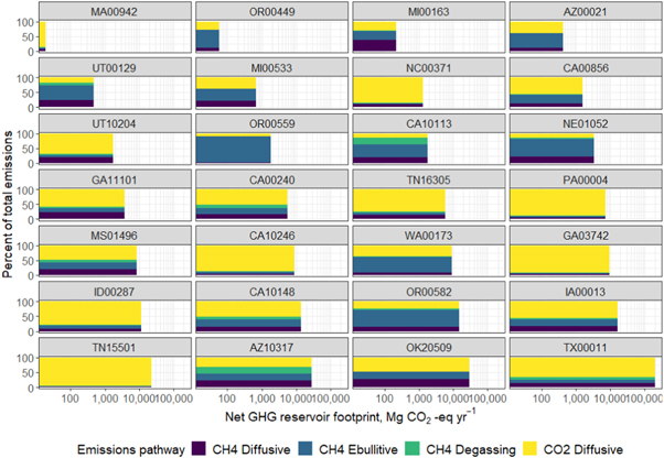
Figure 2. Distribution and magnitude of GHG emissions by reservoir and by pathway. High variability is observed on a per-reservoir basis, as well as across the different emissions pathways. The width of each plot is scaled to total emission while colors represent the percentage of the total reservoir GHG emissions attributed to each pathway. Note the logarithmic scale on the x-axes.
Download figure:
Standard image High-resolution imageA comparison of areal emissions and net generation footprints (total emissions normalized to annual generation) with respect to reservoir size (volume and surface area) highlighted several complexities (figure 3). For example, many of the smaller reservoirs had relatively small generation footprints but some of the largest net areal fluxes (i.e., point labeled C in figure 3). Additionally, the largest net generation footprints were estimated at locations on different ends of the reservoir size spectrum (i.e., points labeled A and B in figure 3). Point A (MA00942) is a small mill structure that was retrofit nearly 30 years after it was built to operate with minimal storage or additional alteration of the non-hydropower releases, while Point B (TX00011) is a major water supply and flood control reservoir. In both cases, hydropower generation is heavily constrained by the other services provided by the dam and the corresponding storage and release rules. On the other hand, Point C (OR00559) was built primarily for hydropower, and generates more energy than other reservoirs even though it is significantly smaller in surface area and volume. This reservoir had one of the smallest generation footprints whereas its areal footprint was the largest of the case-study reservoirs.

Figure 3. Comparison between GHG emission footprints from case-study hydropower reservoirs, normalized with respect to energy generation and surface area. Major differences in footprints with respect to reservoir size (surface area and volume) demonstrate inconsistencies when using size or energy generation as a predictor of GHG emissions. The three labelled points highlight these discrepancies: Point A (MA00942), Point B (TX00011), and Point C (OR00559), which vary greatly in size, purpose, and emission footprints.
Download figure:
Standard image High-resolution imageSuch complex relationships underscore the necessity of considering the range of generation scenarios and constraints that likely exist at multi-purpose reservoirs, particularly where the primary purpose is not hydropower. This is relevant given that common modelling approaches in the literature that have at times used area, generation, or the area to generation ratio as a predictor for GHG emissions (e.g., Scherer and Pfister 2016). For the case-study reservoirs that are included in Deemer et al (2016), modelled post-impoundment areal footprints were positively correlated with measurements reported for all pathways except CO2 diffusion (figure 4). Four of the reservoirs reported negative CO2 diffusion footprints (reflecting uptake of CO2) but the G-res model estimated positive emissions.
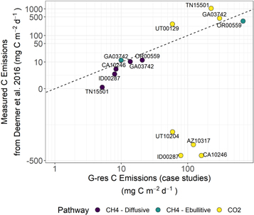
Figure 4. Comparison of G-res modelled areal GHG emissions against measurements reported in Deemer et al (2016) by GHG emission pathway, where data were available. Note log10 transformation of both axes. The dashed line is the 1:1 line. Estimates from the G-res model are generally well correlated (with the exception of CO2 diffusion) and are much higher for all pathways than those measured in the field.
Download figure:
Standard image High-resolution imageTotal areal carbon flux for the case-study reservoirs was highly variable (84 to 767 mg Cm−2d−1, median = 275 mg Cm−2d−1). Comparisons to total measured areal fluxes reported in Deemer et al (2016) are imperfect because measurements often do not include all pathways. However, estimated areal fluxes for the case-studies were on the lower end of the spectrum of measured areal fluxes, which range from −321 to 2150 mg Cm−2d−1 (median = 272 mg Cm−2d−1) for US reservoirs and −355 to 2973 mg Cm−2d−1 (median = 283 mg Cm−2d−1) for global reservoirs.
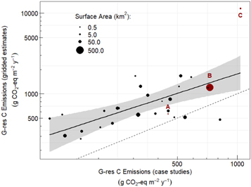
The areal post-impoundment GHG emission footprints of these case-study reservoirs were also positively correlated (Pearson r = 0.81, p < 0.001) with those reported by Harrison et al (2021), though emission estimates from the case-study reservoirs were on average ∼1.6 times lower than the gridded estimates (figure 5). Areal fluxes in the case-study reservoirs were less variable and generally lower than those in the global study, ranging from 138 to 1,052 gCO2eq m−2 y−1, while the global study reported a range of 115 to 145,472 gCO2eq m−2 y−1 (Harrison et al 2021). Differences in the areal emission footprints of methane (US case-study versus US and non-US reservoirs modelled in Harrison et al 2021) were significant (p < 0.001); differences in CO2 were not statistically significant (p = 0.07). These differences are summarized in table S1.
Figure 5. G-res GHG emissions from 28 case-study reservoirs compared to predicted GHG emissions from gridded data from Harrison et al (2021). Point size represents surface area. The solid line is the linear trend line and the dashed line is the 1:1 line. Both axes are log10 transformed. Three points indicated A, B, and C are the same as in figure 3. Gridded predictions overestimated GHG emissions from the case-study reservoirs in nearly all instances.
Download figure:
Standard image High-resolution image
4. Discussion
4.1. Comparison to other modelling and measurement studies
The dominant emission pathways observed in the 28 case-study reservoirs were generally in line with Harrison et al (2021). In both studies, CO2 diffusion and CH4 ebullition were the dominant emissions pathways for hydropower reservoirs across CONUS. There was a difference, however, in the pattern observed at the reservoirs with the greatest total areal fluxes. While case-study reservoirs in the US with the highest areal fluxes were largely dominated by ebullitive CH4 emissions and degassing generally made up a smaller share of the total emissions, Harrison et al found degassing to be the dominant pathway for those reservoirs with the largest areal fluxes.
The median areal carbon flux for case-study reservoirs was consistent with median reported values of mesurements for other US reservoirs and global reservoirs. The areal carbon flux at case-study reservoirs nearly spanned an order of magnitude, but were still concentrated towards the lower range of other US and global reservoirs, despite including all pathways. Negative areal carbon flux were sometimes reported in US and global reservoirs in literature; however, G-res modelled fluxes were never found to be negative. This highlights the limited ability of the G-res model to represent negative post-impoundment fluxes. However, it is important to note that synoptic measurements have their own limitations; a negative flux measured at a single point in space and time may not represent overall conditions in the reservoir.
Gridded estimates of total emissions were consistently greater than those calculated in this study for individual reservoirs. Some differences were expected because the gridded estimates are based on an aggregation and interpolation of reservoirs, so the gridded value may reflect conditions of multiple reservoirs. Additionally, the characteristics of the reservoirs used to produce the gridded estimates differ from those used in this study. For example, the reservoirs used in the global study were generally larger (minimum of 1 km2) and include both hydropower and non-hydropower reservoirs. These differences highlight a limitation of the interpolated values from the gridded dataset; they may represent spatial patterns well, but they may not accurately reflect conditions when downscaled to individual reservoirs.
4.2. Implications for US and global hydropower reservoirs
There are several possible issues with drawing conclusions about regional patterns or the entire US hydropower fleet based on the limited sample of the case-study reservoirs. For example, the underrepresentation of eutrophic systems in the case-study reservoirs compared to global reservoirs could lead to underestimation of emissions. Additionally, case-study reservoirs were younger and larger on average than the broader set of US hydropower reservoirs. Many of the limitations associated with upscaling or extrapolating the case study modelled emission estimates also apply to upscaling of empirical GHG measurements. To address this, one might develop post-stratification methods to assign sampling weights based on reservoir attributes to which G-res is known to be sensitive.
Another important aspect to consider for the larger fleet of US hydropower reservoirs is expected change in catchment development and climate. For example, population increases, urbanization, and anthropogenic catchment activities are all tied closely to reservoir processes through water availability, nutrient and carbon inputs to reservoirs, and changes in reservoir management practices (Ho et al 2017). These factors that could affect carbon cycling and emissions in reservoirs could be exacerbated by compounding effects of changing climate. According to downscaled projections of temperature (Thrasher et al 2013), average annual temperatures will increase at all 28 locations by the end of century under representative concentration pathways 4.5, 6.0, and 8.5 which can impact water availability and catchment vegetation. Additionally, climate is expected to become warmer and drier in many parts of the US, though increased precipitation is expected in the northeastern to upper midwestern US (Beck et al 2018). Many hydropower reservoirs are located in regions where the climate class is expected to change by the end of the century (Hansen, Jackson and DeSomber 2021); potential effects of these changes will need to be considered by reservoir operators and the hydropower community throughout the country as they seek to further understand and mitigate emissions.
Impacts of changing land use, development, and climate can be explored by comparing scenarios or time periods. However, a significant limitation for a non-dynamic statistical modelling approach like G-res is the inability to capture seasonal or year-to-year variation. In reality, variation can impact GHG production and emissions. Climate and environmental changes resulting in warming could affect a variety of lake processes including thermal stratification, which is a critical control on carbon processing, but which the G-res model does not capture in a dynamic fashion. Internal carbon processes and feedbacks can be complex during stratified periods, which have become longer (Woolway et al 2021) and stronger (Kraemer et al 2015, Pilla et al 2020) in lakes and reservoirs around the world (Sobek et al 2009, Carey et al 2018). Longer and stronger stratification can lead to longer periods of low oxygen at depth (Fang and Stefan 2009, Foley et al 2012, Rösner, Müller-Navarra and Zorita 2012, Knoll et al 2018) that promotes CH4 production. Additionally, both the production and subsequent decomposition of algae is exacerbated by warming (Visser et al 2016). This response also contributes to low oxygen in deep waters that promotes CH4 production and has been highlighted as an important driver of CH4 emissions at a global scale (Sepulveda-Jauregui et al 2018, Beaulieu, DelSontro and Downing 2019). While reduced oxygen in deep regions of lakes and reservoirs is a pervasive pattern globally, there is high variability in both the rate and drivers of change (Jane et al 2021). This variability over space and through time makes it challenging to quantify GHG emissions within reservoirs. Use of physically-based models or process representation in statistical models will enable better understanding of emissions over time and across different bodies of water.
In addition to process variability that is not yet captured by the G-res model, there may also be uncertainties in key characteristics that lead to uncertainty in modelled emissions. For example, reported reservoir volumes or depths may differ from one reservoir or dam inventory to another, depending on the resolution or method used to determine the characteristic. A formal sensitivity analysis that considers uncertainty and quality assessments of the inputs is needed to determine how these uncertainties impact modelled results.
5. Conclusion
Comparisons between case-study modelled GHG emissions and measurements or modelled emissions from other subsets of reservoirs highlight where there is consistency in observed patterns or where there may be limitations in describing individual reservoirs. Trends in GHG emissions pathways at the case study hydropower reservoirs are generally consistent with those observed across global scales with CO2 diffusive fluxes dominating the overall GHG footprint for the majority of the reservoirs. Comparisons also provide context for how US hydropower against to other subsets of reservoirs. While there was general agreement between estimates and measurements for most pathways, there were several instances where possible carbon sinks were not well represented by the G-res model. Additionally, while estimates of net footprints were highly correlated with those extrapolated from estimates at larger reservoirs modeled in other studies, they were consistently lower across the smaller and diverse multi-purpose case-study reservoirs.
While degassing caused by deep water intakes was not the dominant pathway for emissions at any of the case-study reservoirs (unlike the largest emitters in the global G-res study), it did account for a substantial portion of emissions at several of the reservoirs and remains an important opportunity for reducing GHG emissions. Limitations in representing intake depth dynamically (due to static representation of intake depth in the model) may be overcome with additional data collection and scenario-based modeling to evaluate design and operational strategies. Additionally, even in empirical GHG measurements, the degassing pathway is very understudied compared to other emissions pathways. Greater focus on measuring this pathway may reduce the uncertainties in future modelling efforts. Understanding these mechanisms will require extending analyses by including more detailed representations of catchment hydrology and human/reservoir management interface and considering policies, water rights, multi-purpose uses of the water, and not solely water availability or operational strategies.
GHG emissions from waterbodies are a critical part of the global carbon equation. Accurate representations of GHG footprints (and their contributing factors) at hydropower reservoirs are especially important to enable evaluation of environmental tradeoffs during the transition away from fossil fuel and ensure emissions reduction targets are met. Especially when these waterbodies are often managed for various purposes, more detailed and accurate reservoir GHG emissions footprints can lead to better identification of where monitoring and mitigation resources could be allocated, and which strategies could be employed to reduce reservoir emissions.
Acknowledgments
The authors recognize the G-res tool development team, including Sara Mercier-Blais, for producing thorough documentation of the tool and its underlying models. We thank Kristine Moody for her review and suggestions for improving the manuscript.
Data availability statement
All data that support the findings of this study are included within the article (and any supplementary files).
Funding
This manuscript has been authored by UT-Battelle, LLC, under contract DE-AC05-00OR22725 with the US Department of Energy (DOE). The US government retains and the publisher, by accepting the article for publication, acknowledges that the US government retains a nonexclusive, paid-up, irrevocable, worldwide license to publish or reproduce the published form of this manuscript, or allow others to do so, for US government purposes. DOE will provide public access to these results of federally sponsored research in accordance with the DOE Public Access Plan (http://energy.gov/downloads/doe-public-access-plan).