
Abstract
Corrosion of the piping system is a genuine problem in the oil and gas industry. Most oil and gas industries used a carbon steel pipeline for the transportation of crude oil, which is affected by CO2 corrosion. Now a day, the computational approach and artificial neural network approach will be used to study the corrosion rate. Therefore, in this work, Computational Fluid Dynamics (CFD) and Artificial Neural Network (ANN) studies on piping systems were made to determine the corrosion rate induced by CO2 saturated aqueous solutions on carbon steel pipeline. In CFD study, corrosion rates were computed by modeling the electrochemical processes occurring at the metal substrate from cathodic reductions of the carbonic acid and hydrogen ions, and the anodic oxidation of the metal component. Also, an artificial neural network study was made using a multilayer perceptron neural network method; and, computational fluid dynamics and artificial neural network simulations were validated with in-house built experiment set-up. The experimental study had been carried out for more than 200-h to find the corrosion rate on the pipeline, and satisfactory trends were observed between computational fluid dynamics, artificial neural network, and experimental values. In the end, corroded pipes were observed under a scanning electron microscope and x-ray spectroscopy, and the corroded zones were viewed as against the non-corroded pipe.
Export citation and abstract BibTeX RIS
Introduction
Corrosion is the deterioration and loss of a material due to the destructive attack of a metal by its reaction with the environment. Most of the oil and gas industries are suffering from corrosion-related problems. Kermani and Harrop's [1] study highlighted about 25% of failures in the oil and gas industries were because of corrosion, and CO2 corrosion is the main type of corrosion which caused the failures. Many researchers had been proposed different models to estimate the corrosion rate [2–4]. However, regardless of all the developments, predicting the corrosion rate and controlling its harmful effects is still a challenging task. Earlier studies and field experiences revealed that predicting the internal flow behavior is essential in developing a predictive corrosion model, and eliminating the hazardous effects of internal corrosion [5–7].
A predictive model was developed for CO2 corrosion from modeling individual electrochemical reactions in a water-CO2 system [8] and the performance of the model was validated by comparing the predicted results from experimental values. The study results indicated that the model gave a better understanding of the corrosion mechanisms by considering the effects of pH, temperature, and flow rate. Srinivasan [9] developed a numerical model for computing corrosion rates generated by CO2 saturated aqueous solutions for the pipe flow. The corrosion model was validated at different pH, flow velocity, pressure and temperature conditions. In addition, flow variations induced by geometrical non-uniformity were studied to know the hydrodynamic variations in the corrosion predictions.
Nesic [10], Nesic and Carroll [11] and Li et al [12] concentrated on the characteristics of water wetting (water with CO2 and H2S gases). Their study indicated that water wetting at the bottom of steel pipe due to the higher density of water compared to the oil and the corrosion rate in the pipelines is dependent on the wetted area. Jiyong et al [13] carried out an experimental study of oil-water flow for flow pattern visualization and monitoring of corrosion rate. The study of the ferrous ion monitoring demonstrated that when water wets the pipe walls the corrosion occurs and it is greater for stable water wetting than for intermittent wetting. Similarly, Li et al [14] carried out investigations using electrochemical measurements and computational fluid dynamics (CFD) simulation for the main causes of the corrosion in X65 pipeline steel when the pipelines were saturated with CO2 and oil-water emulsions. Their study highlighted that the rate of corrosion was affected by parameters like flow velocity, temperature and the content of oil in the fluid.
In addition, several researchers have studied the ANN approach while predicting the corrosion rate. Kamrunnahar and Urquidi-Macdonald [15] used a neural network (NN) method as a data mining tool to predict the corrosion behavior of metal alloys. In their study, experiments data on corrosion allowable and resistive alloys were collected and data mining results were allowed to prioritize the parameters like pH, temperature, time of exposure, electrolyte composition, metal composition, etc on electrochemical potentials and corrosion rates. Also, Giulia et al [16] made a case study to properly predict the presence of metal loss and corrosion rate along a pipeline from the field data. In their ANN model, geometrical features, fluid dynamics variables, and corrosion models were considered and the study showed all three components play an important role in network training and simulation. Also, Bassam et al [17] proposed a neural network model that could predict the corrosion in pipeline steel as a function of inhibitor concentration and time. In their study, a neural network model was successfully trained with experimental values. Mazura Mat Din et al [18] developed a time-dependent corrosion growth model for the oil and gas pipeline using Artificial Neural Network (ANN). The developed ANN model could be able to predict the corrosion rate based on in-line inspection data (ILI), corrosion depth and length of the defect.
From the above literature reviews, it has emerged that CO2 corrosion is purely chemical kinetics and hydrodynamics driven, and therefore, CFD and ANN analysis on CO2 corrosion is of great importance to predict the corrosion rates. Moreover, from the literature, it was confirmed that combined CFD and ANN comparative study on CO2 corrosion has not been performed and very limited research work on CO2 corrosion with CFD kinetics is also available. With this thought, in this study, the CO2 corrosion on the pipeline was performed with different operating conditions. The CFD analysis was performed to observe chemical kinetics and hydrodynamics to develop a generic framework to compute corrosion rates, and results were validated with experimental values. Furthermore, the ANN approach was developed from Multilayer Perceptron Neural Network (MLPNN) to predict the corrosion rates of the pipeline under different operating conditions.
Modeling and simulation
The corrosion rate is generated by the interaction of aqueous CO2 solution with the metallic surface due to chemical reactions. In general CO2 hydration is a slow chemical reaction; a small amount of carbonic acid is dissociated into the hydrogen ion, bicarbonate, and carbonate ions. The study of CO2 corrosion in a piping system is an electrochemical process that involves the anodic dissolution of carbon steel and cathodic evolution of hydrogen. The overall reaction can be written as:
A small fraction of the dissolved CO2 reacts with water to give carbonic acid.

In addition, carbonic acid undergoes dissociation in two steps, equations (2) and (3). These reactions are very fast and contribute corrosion of steel, thus maintaining chemical equilibrium.


In the current study, H+ and H2CO3 are the two cathodic reactions being considered and H+ and H2CO3 species are transported to the species conservation equation to calculate the convection and diffusion transport. In addition, H+ and H2CO3 reduction mechanism is also mass transfer limited and is considered in the corrosion modeling process.
Anodic and cathodic reactions of CO2 corrosion
The electrochemical corrosion of the steel surface is represented by one anodic and at least one cathodic reaction. The anodic reaction in carbon dioxide corrosion is represented by

Moreover, the presence of CO2 increased the rate of corrosion of steel in aqueous solution by increasing the rate of hydrogen evolution as per,

Also, the direct reduction of H2CO3 could increase the corrosion rate,

In addition, the direct reduction of the bicarbonate ion becomes significant at pH greater than 5

CO2 corrosion rate estimation
CO2 corrosion of the steel surface is the electrochemical corrosion, and oxidation of iron is the main anodic reaction. The overall corrosion behavior is dependent on H+ ions transported from the solution to the corroding metal interface. As per the Butler-Volmer equation, the electrochemical reaction rate depends on the temperature and exchange current density of the anodic and cathodic reactions [19].
The oxidation of iron at the corrosion potential is charge transfer control and corrosion potential for the anodic reaction represented as

Where io is the exchange current density, ba is Tafel slope, Ecorr is corrosion potential and Erev is the reversible potential of iron oxidation.
Similarly, H+ and carbonic acid reduction reaction is dependent on charge transfer and mass transfer (diffusion) control and can be represented as

Where  charge transfer current density and
  is the diffusion limit current density for the cathodic reaction
Also, the charge transfers the current density of the H+, H2CO3 reactants is calculated from Tafel's equation,

Where bc is Tafel slope for the cathodic reaction
The reversible potential, Erev(R) is used to calculate the exchange current density and is computed from pH and temperature, T

Where n is no. of electrons transferred and F is Faraday's constant
Moreover, the reduction mechanism of the species H+ and H2CO3 is mass transfer limited and diffusion limit charge current, idlim(R) is determined from

Where km is the diffusion coefficient and Y is the species concentration. In the present study, empirical correlations were used to calculate the mass transfer coefficients.
The corrosion potential will be solved from mixed potential theory, from which corrosion current is estimated and using Faraday's law corrosion rate is estimated.
CFD modeling
The Navier–Stokes equations of mass, momentum, energy, and species model were considered in CFD study. To capture the turbulent fluctuating components of fluid velocity, pressure and other species, a set of Reynolds-Averaged Navier–Stokes equations were assembled in the simulation. In the current work, a more reliable k-ω Shear-Stress Transport (SST) model had been applied to determine the near-wall viscous sub-layer established during a turbulent flow. The Shear Stress Transport (SST)  model effectively blends the robust and accurate formulation of the
  model in the near-wall region with the free-stream independence of
  model in the far-field.
Species model
In the species model, reaction rates were determined by general finite-rate chemistry and the effects of turbulent fluctuations on kinetics rates were neglected. When no turbulence-chemistry interaction (TCI) model was used, the finite-rate kinetics was incorporated by computing the chemical source terms using general reaction-rate expressions. This approach is recommended for laminar flows, where the formulation is exact. However, for the turbulent flows, the turbulence time-scales were used in a relative to the chemistry time scales using complex chemistry.
The net source of chemical species due to reaction, Ri, is computed as the sum of the molar rate of creation or destruction of species in the reaction,

Where Mw,i is the molecular weight of species; and Ri,R is the molar rate of creation/destruction of species, i, in reaction, R.
The molar rate of creation/destruction of species in reaction, Ri,R is given by

Where, N is number of chemical species in the system;  and
and  are the stoichiometric coefficient for product and reactant, i, in reaction R;
  and
and  is forward and backward rate constants for reaction, R; Cj,R is molar concentration of species in reaction R;
  and
and  are rate exponent for reactant and product species in reaction R. Moreover, Γ represent the net effect of third bodies on the reaction rate and is not considered in the reaction rate calculation. Also, the forward rate constant for reactions,
  is computed using Arrhenius expression.
CFD methodology
ANSYS - 18.1 software was used to simulate the pipeline corrosion rate when a fluid flows with a certain quantity of species. The simulations were performed to determine the corrosion rate from initializing the model with inlet boundary conditions for varying pH values of carbonic acid. Moreover, the in-built E-Chem reaction model of [20] was used to perform the simulations. In the analysis, Butler-Volmer parameters for anodic and cathodic reactions and species charge numbers were incorporated in the species model. Also,  SST viscous model was used for the turbulence behavior of the flow which considered the near wall and far-off effects to model the wall-bounded flows and free-shear flows in the domain.
A second-order discretization scheme was used for pressure, momentum, turbulence, species and energy variables study. The simulation studies were carried out for steady and transient state conditions. Moreover, the effect of wall roughness and heat generated by the species interactions were not considered, since no details were available in the present experimental study.
Model geometry and grid details
In this study, a three-dimensional hexahedral meshing of the pipeline was created in ANSYS Workbench 18.1. The electrochemical reactions of anodic and cathodic reactions were solved numerically in ANSYS Fluent 18.1 to define the CO2 corrosion rate. Also, independent grid elements were used to model the flow within the geometry and the accuracy of grid size was observed by performing a grid-independent convergence. Moreover, structured grid structures (hexahedral type elements) had been implemented along with the flow domain. A 30 cm length and 12.7 mm diameter carbon steel pipe was chosen to study the CO2 corrosion. Figure 1 shows the model and meshed geometry of the pipeline domain.

Figure 1. Pipeline geometry—3D model and meshed geometry.
Download figure:
Standard image High-resolution imageThe wall-bounded turbulent flows were meshed using inflation layer meshing to accurately capture the boundary layer region. Table 1 highlights the mesh details of the studied pipe.
Table 1. Mesh details for the studied pipeline.
| No. of nodes | 209 760 |
| No. of Faces | 616 041 |
| No. of Cells | 203 196 |
| Type of elements | Hexahedral element |
| Maximum aspect ratio | 206 |
| Minimum orthogonal quality | 0.572 |
Boundary conditions
The Butler-Volmer/Tafel parameters like exchange current density, equilibrium potential, and anodic and cathodic Tafel slope need to be specified for every E-Chem reaction. The typical values used for pH 4 simulations are indicated in table 2 (Mohammad [21]).
Table 2. Summary of boundary conditions.
| Tafel slope, volt/decade—electrochemical reactions | |||
|---|---|---|---|
| pH | Fe oxidation | H + reduction | H2CO3 reduction |
| 4 | 0.04 | 0.118 | 0.12 |
| Exchange current density, amp m−2 | |||
| pH | Fe oxidation | H + reduction | H2CO3 reduction |
| 4 | 1.69 | 0.041 | 0.219 |
Artificial neural networks
Artificial neural networks are computing systems based on artificial neurons, which can transmit the signal from one neuron to another. In the current work, the Multilayer Perceptron Neural Network method was used to predict the CO2 corrosion in the pipeline. The selection process of several data points for training, testing and validation will be carried out automatically in MATLAB-NNTOOL.
Multilayer perceptron neural network (MLPNN)
Multi-layer perceptron's are the most useful type of neural network and the analytical capability of neural networks comes from the multi-layered structure of the networks. The data structure can learn to represent features at different resolutions and combine them into higher-order features.
MLPNN consists of four neurons in the input layer corresponding to four input parameters (pH, pCO2, velocity, and temperature) in this study. The output layer consists of a single neuron, which is corrosion rate as an output parameter. A single hidden layer with Nh (number of hidden neurons) was used in this work which will hold weights and biases in the hidden layer (Wij, bij) and an output layer (Wjk, bjk) as shown in figure 2. Sigmoidal activation function was selected to link between inputs and output. For training purposes, the back-propagation (BP) algorithm was used in MLPNN. Gradient descent with momentum and adaptive learning rate back-propagation (gdx) was used due to its ability to update weights and biases. Also, other factors like learning rate (γ) and momentum rate (μ) were chosen and the performance of MLPNN was validated through MSE (Mean Square Error). The learning rate parameter was used during the adjustment of weights and biases to control the speed of learning algorithm and activation functions (hyperbolic tangent sigmoid and log-sigmoid).

where y is the net of input values and targets expected output value.

Figure 2. Structure of MLPNN.
Download figure:
Standard image High-resolution imageThe structure of the MLPNN is shown in figure 2.
Experimental setup
The experimental set-up was built in-house to validate the CFD results, and the set-up has a carbonic acid storage tank, pressure gauges, valves, water pump, and pipe specimen. An electrical automatic water pump of 11 lpm capacity was chosen in the current work and mechanical pressure gauges were used to determine the pressure drop across the pump. A carbon steel pipe test specimen of 300 mm length and 12.7 mm diameter was assembled to the setup and the carbonic acid flow is regulated through the mechanical valve.
In the current study, the carbonic acid concentration is fixed by bubbling (passing) the CO2 gas in the water under controlled condition and the amount of dissolved CO2 changes the concentration of carbonic acid. In the study, 1 bar partial pressure is maintained for CO2 and pH meter is used to verify the pH value of carbonic acid. In the beginning, carbonic acid solution pH 4 was prepared, and the experimental study was carried out for 200 h to estimate the CO2 corrosion. A later stage, distilled water was added to the solution to change the pH value, and the study had been carried out for pH 5 and 6. Besides, the flow velocity of the fluid was maintained as 0.9 m s−1 through a mechanical valve and the experimental test set-up is shown in figure 3.

Figure 3. Experimental set-up.
Download figure:
Standard image High-resolution imageIn each case, the corrosion rate was determined through the weight loss method and the studied pipe specimens were observed under scanning electron microscopy and also, energy dispersive x-ray spectroscopy approach was used to identify the composition of corrosion film.
Weight loss method
Simplest method to predict the corrosion wear. In this method, the weight of the pipe is determined at the end of an experiment and the loss in weight signifies the corrosion wear.
Scanning electron microscope
In the current work, the Scanning Electron Microscope study on the samples was carried out at the Central Analytical and Applied Research Unit (CAARU), Sultan Qaboos University, Sultanate of Oman. The engaged SEM setup had high power optics irradiation system with an integration of a gentle beam that enables top-surface imaging of a specimen at very low energies and possible to obtain high-resolution images of samples. The model name of the employed SEM unit is JSM-7600F Schottky Field Emission Scanning Electron Microscope, Jeol Company, Japan.
Results and discussion
Flow behavior
The flow behavior in a pipe specimen was studied using CFD for varying the velocities from 0.5 m s−1 to 1.5 m s−1. Figure 4(a) explains the velocity contour plots for the 0.9 m s−1 velocity and pH 4. The study results revealed that fully developed turbulence is encountered in the bulk fluid and as the fluid approached the solid wall, turbulent fluctuations were dampened and negligible velocity was noticed at the wall. Also, a Schmidt number value of 504 was noticed for the flow, and it showed that the mass transfer boundary layer is very small in the flow.
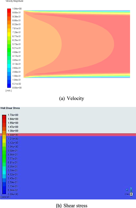
Figure 4. Contour plots of velocity and shear stress for pH 4 condition.
Download figure:
Standard image High-resolution imageIn addition, shear stress exerted at the wall is highlighted in figure 4(b) and in the CFD simulation, a maximum shear stress value of 1.73 Pa was noticed at the wall surface for 0.9 m s−1. However, analytical calculations showed a stress value of 2.45 Pa for 0.9 m s−1. The variation in stress values could be due to in CFD simulation CO2 corrosion species densities were considered as against the carbonic acid density in the analytical calculation. Furthermore, the analytical study results also indicated that with increase in velocity the wall shear stress augmented because of the rise in the velocity head across the flow path and also it enhanced the friction at the wall surfaces as highlighted in figure 5. The analytically calculated shear stress values for change in the velocity curve indicated the R2 value of 0.99 and the observed shear stress values lies within 20% range from the best-fitted curve.

Figure 5. Shear stress variations with respect to flow velocity.
Download figure:
Standard image High-resolution imageEffect of pH on corrosion rate
To understand the mass transfer behavior of the species at pH less than 5 were important in the CO2 corrosion mechanisms study. In this regard, the mass transfer characterization of a chosen pipe was made using CFD and the structured mesh was used in the simulation. Moreover, nearly 15 boundary layers were used to resolve the viscous sub-layer for the description of species distribution across the pipe length. Also, for the entire CFD simulations only one type of computational mesh was exercised based on the flow conditions. In the simulations, aqueous solution temperature was maintained at 25 °C and solution pH concentrations were varied to understand the CO2 corrosion on the pipeline. The study results highlighted that a large contribution of H+ reduction could be seen at pH 4 and this influence gets diminished at pH 5 and 6. Figure 6(a) explains the concentration of H+ ions and maximum mass fraction of 0.0003 is noticed at the boundary layer of the pipe wall surface for pH 4 and 0.9 m/s flow. However, with the diluted carbonic acid (as pH increased) the concentrations of H+ ions at the wall boundary is more and it led to lower the H+ reduction reaction as indicated in figure 6(b) for pH 6 and 0.9 m s−1 velocity. Furthermore, the CO2 corrosion study revealed that at pH 5 and 6, the dominant cathodic reaction at the corrosion potential will be H2CO3 reduction.

Figure 6. Contour plots of H+ species.
Download figure:
Standard image High-resolution imageFigure 7 explains corrosion behavior in the pipe at different pH concentrations for the 0.9 m s−1 flow velocity. At pH 4 concentrations the observed corrosion rate value was 5.41 × 10⁻⁷ kg m−2-s and is equal to 2.05 mm year−1. However, at pH 5, very negligible corrosion was noticed on the pipeline. This is because the concentration of the H+ and H2CO3 species at the wall surface for pH 5 is less as compared to pH 4. Similarly, the current density for iron oxidation is very negligible for pH 5 concentration.

Figure 7. Variation of corrosion rate with different concentrations of pH.
Download figure:
Standard image High-resolution imageFurthermore, at pH 6, very low corrosion was noticed on the pipe surface, and it could be due to a completely diminishing H+ reduction reaction with an increase in pH concentrations. Overall, the study confirmed that H+ reduction and current densities were the dominant parameters in CO2 corrosion for pH values less than 5. However, at pH6, negligible corrosion traces were noticed on the pipeline surface because of the reduction of the bicarbonate ion which forms a protective iron carbonate film on the surface and decreased the CO2 corrosion on the pipeline.
Effect of flow velocity on corrosion rate
In addition, simulation studies had been carried out with varying flow velocities from 0.5–2 m s−1. In the simulation study, a pH 4 was used to understand the effect of fluid convection on the corrosion rate. The careful assessment of mesh at the entrance length in the pipe and boundary layer zone (wall) is important to understand the turbulence behavior for different flow velocities. Hence, in the current study to reduce the computational mesh generation for various flow conditions the structured grid with a y+ approximately 1 was used.
Figure 8 explains the corrosion rates plot for different velocities. As velocity was increased, the limiting current for H+reduction augmented and led to an increased overall cathodic reaction and enhanced the corrosion rate. At higher velocities, the flow-dependent H+ reduction was dominant as the concentration of H+ species was maximum. The study results confirmed that at 2 m s−1 the maximum corrosion value of 6.30 × 10⁻⁷ kg m−2-s was observed and is equal to 2.53 mm year−1. The plotted curve indicated the 0.999 R2 value and the observed corrosion rate values lie within a 10% range from the best-fitted trend line. Moreover, study results highlighted that for the same velocity with an increase in pH concentrations negligible corrosion was noticed because of limited H+ ions in the solution and small contribution to raise in the cathodic current.

Figure 8. Corrosion rate with respect to different flow velocities for pH = 4.
Download figure:
Standard image High-resolution imageEffect of time on corrosion rate
The simulation was carried out under transient conditions to identify the significance of testing time on the corrosion rate. In the analysis, the fluid flow velocity of 0.9 m s−1 and the pH 4 were considered. Figure 9 highlights the variation of corrosion rate with respect to time and the study results revealed that until 2500 s, the corrosion rate values were decreased from 8.97 × 10⁻⁶ kg m−2-s to 5.7 × 10⁻⁷ kg m−2-s. This could be due to the species diffusion through the boundary layer is more in the beginning and it enhanced the corrosion rate. However, at the later part of the simulation, almost stable corrosion of 2 × 10⁻⁷ kg m−2-s was observed for the 5-h run. This could be due to a decrease in species diffusion through the boundary layer, and also H+ reduction and limiting current for cathodic reactions were time-independent and will be the same throughout the simulation.

Figure 9. Variation of corrosion rate with respect to time (pH 4 and 0.9 m s−1 case).
Download figure:
Standard image High-resolution imageExperimental study
In the present work, CO2 corrosion experiments on the pipeline were carried out for different pH concentrations of carbonic acid varying from 4 to 6. In the experimental study, fluid temperature and flow velocity were maintained as 25 °C and 0.9 m s−1 respectively. For each case, experiments were carried out for 200 h and the corrosion rate was determined from the weight loss method. Refer table 3 for the calculated corrosion rate values for different pH values and at pH 4 about 2.08 mm\year corrosion was noticed.
Table 3. Experimental results of CO2 corrosion.
| Sl. No. | pH | Fresh pipe weight, g | Pipe weight after corrosion, g | Weight loss, g | Corrosion rate, mm\year |
|---|---|---|---|---|---|
| 1 | 4 | 0.170 | 0.168 790 | 1.210 × 10⁻³ | 2.08 |
| 2 | 5 | 0.170 | 0.169 975 | 0.0255 × 10⁻³ | 0.03 |
| 3 | 6 | 0.170 | 0.169 99 | 0.0100 × 10⁻³ | 0.01 |
In addition, at pH 5 and 6, the observed corrosion rate was very negligible. This could be due to a decrease in H+ species in the carbonic acid which reduced the tendency of Fe2+ to diffuse from the surface and finally diminished the corrosion on the wall surface.
Moreover, the SEM image of the cross-section of a specimen before the start of the experiment is indicated in figure 10 and the smooth surface was witnessed.

Figure 10. SEM image of non-corroded pipe.
Download figure:
Standard image High-resolution imageAlso, figure 11 represents the x-ray spectroscopy plot of a specimen before the start of the experiment. The study indicated small peaks of Fe, C and O compound in the specimen and no oxide formation on the surface.

Figure 11. Energy-dissipative x-ray Spectroscopy spectra of non-corroded pipe.
Download figure:
Standard image High-resolution imageFigure 12(a) highlights the SEM image of the tested sample for 200 h at pH 4 and 25 °C and flow velocity of 0.9 m s−1. The image results revealed that corrosion films on the surface were dense and the film witnessed laminated and fractured corroded surface and it confirmed that the presence of diffusion-controlled processes in the corrosion mechanism of the steel pipe surface. The image represented the corrosion products in dark color, while the steel pipe base metal appearing as white color.

Figure 12. SEM images of corroded pipe.
Download figure:
Standard image High-resolution imageMoreover, SEM images for pH 5 and 6 are indicated in figures 12(b) and (c). For the pipe specimens corresponding to pH 5 and 6, and evenly attacked surface and very small thin films could be seen on the surfaces. However, at pH 5 case slightly more corrosion was noticed on the surface as compared to pH 6. The decrease in CO2 corrosion on the pipeline with pH 6 is due to an increase in the formation of a protective iron carbonate film as compared to pH 5 cases. Thus, the SEM study confirmed that the CO2 corrosion process on the pipeline was mass transfer controlled at lower temperatures and low flow velocity. Furthermore, at low pH values, the surface films were porous and allowed the species to diffuse in the film, and enhanced the corrosion of the surface.
Moreover, the x-ray spectroscopy plot of a corroded pipe for pH 4 is highlighted in figure 13. The study results revealed that high peaks of Fe, C, and O on the corroded specimen. The C peak is mainly associated with an iron carbide matrix filled with iron carbonate on the corrosion area. Thus, an x-ray spectroscopy plot confirmed that high concentration of Fe oxidation in the wall surface for pH 4.

Figure 13. Energy-dissipative x-ray spectroscopy spectra of corroded pipe: pH = 4.
Download figure:
Standard image High-resolution imageANN results
As mentioned earlier, MATLAB-NNTOOL was used to predict the corrosion rate using a neural network approach. The study results indicated that gradient, validation check, and learning rate values were 0.033 887, 10 and 0.022 92 respectively at epoch 17 for the training data of MLPNN. Additionally, mean square error results highlighted the best validation performance of 0.000 906 59 at epoch 7 and a small error value between training, validation and testing data.
Figure 14 shows the linear regression between training, validation, and testing of the MLPNN model. From the figure, it is confirmed that the target line ratio of the MLPNN model almost matched the experimental results and demonstrated that the predicted values were close to experimentally measured value under the same operating conditions. Also, ANN results confirmed that there was an excellent linear relationship between the output value and experimentally observed value. The optimal MLPNN configuration obtained was 4-5-1 (five neurons in Nh) with learning rate and momentum rate values of 0.022 92 and 0.0025 respectively.

Figure 14. Linear regressions of predictions and targets of MLPNN method.
Download figure:
Standard image High-resolution image
Comparison of corrosion rate—CFD, experiment and ANN results
Experimental results of corrosion rate were compared with CFD and ANN analysis and close agreement were observed for flow velocity of 0.9 m s−1 as indicated in table 4. An error of 1.44% was observed between CFD and experimental results for pH 4 conditions. Moreover, for pH 5 and 6 cases, the experimentally observed corrosion values were very less and the same trend was observed with CFD simulation. Furthermore, a close agreement was observed between experimentally observed values and the MLPNN approach for the case of pH 5 and 6. On the whole, from this study, it is confirmed that boundary conditions adopted in CFD analysis, and also ANN training, validation and testing approaches were accurate to predict the CO2 corrosion in the pipeline for different conditions.
Table 4. Comparison of experimental results with CFD and ANN analysis.
| pH | CFD analysis, mm year−1 | Experiential results, mm year−1 | MLPNN prediction mm year−1 |
|---|---|---|---|
| 4 | 2.05 | 2.08 | 2.045 |
| 5 | 0.029 | 0.03 | 0.031 |
| 6 | 0.0095 | 0.01 | 0.012 |
Conclusions
The following are the outcomes of the present work:
- The electrochemical corrosion with the carbonic acid flow in the steel pipeline was successfully studied to investigate the CO2 corrosion. The study results confirmed that CO2 induced corrosion rate in the pipeline was mass transfer limiting current of H+ ions for the pH 4 conditions.
- Experiments were carried out for 200 h at different pH values to validate the CFD results. An error of 1.44% was noticed between CFD and experimentally observed corrosion results for the case of pH 4.
- SEM and x-ray spectroscopy study for the fresh and corroded pipes were carried out, and corroded pipe showed more material detachment from the surface for pH value of 4 and negligible corrosion with pH 5 and 6 cases.
- ANN study results indicated that predicted values were almost near to experimentally observed corrosion values under the same operating conditions.
- On the whole, CFD, ANN, and experimental approaches were successfully used in the current work and the study gave valuable thoughts on CO2 corrosion in the pipeline.