
Abstract
To make progress in science, we often build abstract representations of physical systems that meaningfully encode information about the systems. Such representations ignore redundant features and treat parameters such as velocity and position separately because they can be useful for making statements about different experimental settings. Here, we capture this notion by formally defining the concept of operationally meaningful representations. We present an autoencoder architecture with attention mechanism that can generate such representations and demonstrate it on examples involving both classical and quantum physics. For instance, our architecture finds a compact representation of an arbitrary two-qubit system that separates local parameters from parameters describing quantum correlations.
Export citation and abstract BibTeX RIS

Original content from this work may be used under the terms of the Creative Commons Attribution 4.0 license. Any further distribution of this work must maintain attribution to the author(s) and the title of the work, journal citation and DOI.
1. Introduction
Neural networks are among the most versatile and successful tools in machine learning [1–3] and have been applied to a wide variety of problems in physics (see [4–6] for recent reviews). Many of the earlier applications have focused on solving specific problems that are intractable analytically and for which conventional numerical methods deliver unsatisfactory results. Conversely, neural networks may also lead to new insights into how the human brain develops physical intuition from observations [7–14].
Recently, the potential role that machine learning might play in the scientific discovery process has received increasing attention [15–22]. This direction of research is not only concerned with machine learning as a useful numerical tool for solving hard problems, but also seeks ways to establish artificial intelligence methodologies as general-purpose tools for scientific research.
An important step in the scientific process is to convert experimental data, which can be seen as a very high-dimensional and noisy representation of a physical system, into a more succinct representation that is amenable to a theoretical treatment by a human user. For example, when we observe the trajectory of an object, the natural experiment is to record the position of the object at different times; however, our theories of kinematics do not use time series of positions as variables, but rather describe the system using quantities, or parameters, such as initial velocity and initial position. The description of a system in terms of initial velocity and initial position is both succinct and operationally meaningful since the concept of velocity by itself can be used to perform prediction tasks in many different physical settings. If we instead described the system by e.g. the sum and difference of initial velocity and initial position (in some fixed units), this would still succinctly represent the same information, but it would not be operationally meaningful and mostly useless to a human interpreter. This is because the sum of initial velocity and initial position by itself is generally not a useful quantity for making predictions. This notion is motivated by the following general criterion for physical theories. We want a theory to describe a system in such a way that if different agents perform different experiments on a systems, they only need to know a subset of the parameters describing this system. We call this criterion efficient communicability: we imagine that one agent has a full description of the system in terms of a set of parameters and wants to tell other agents about the aspects of the system relevant to their experiments by sending a subset of parameters. Then, the parameters describing the full system should be chosen in such a way as to minimize the required communication.
In this work, we formally introduce the concept of operationally meaningful representations and present a neural network architecture for the automated discovery of such representations. To this end, we define an operationally meaningful representation of a physical system as the minimal set of parameters that describes the full system such that each parameter is relevant for different experiments one can actually perform on the system. In line with this definition, we design a neural network architecture that can generate a meaningful representation through an attention mechanism. We demonstrate that this architecture can indeed identify parameters such as charge, mass, or even amplitudes of a quantum state in an operationally meaningful way from high-dimensional experimental data.
2. Operationally meaningful representations
The field of representation learning is concerned with feature detection in raw data. While, in principle, all deep neural network architectures learn some representation within their hidden layers, most work in representation learning is dedicated to defining and finding good representations [23]. A desirable feature of such representations is the interpretability of their parameters (stored in different neurons in a neural network). Standard autoencoders, for instance, are neural networks which compress data during the learning process. In the resulting representation, different parameters in the representation are often highly correlated and do not have a straightforward interpretation. A lot of work in representation learning has recently been devoted to separating or disentangling such representations in a meaningful way (see e.g. [24–28] and appendix
When using neural networks to find such parameterisations, one encounters the limitation of standard techniques from representation learning: typically, statistically independent factors of variation in the training data set are disentangled. That is, disentanglement arises implicitly from the statistical distribution of the data set. This works well for many practical problems [24]; however, for scientific applications, it is desirable that parameters be separated according to a more fundamental and transparent criterion than the distribution of experimental data.
To this end, we introduce operationally meaningful representations. In such a representation, parameters that are useful for different operational tasks on a physical system should be stored in separate neurons. As an example, take the physical system to be a charged mass. We consider a situation where one agent E has performed a data collection experiment so that this agent has a high-dimensional representation of all potentially relevant information about this system, e.g. its mass, charge, and colour. Other agents want to predict the outcome of various evaluation experiments on this charged mass (their 'operational task'), e.g. colliding it with another (uncharged) mass or placing it in an external electric field. For this, these agents will receive information about the system from agent E. The key restriction is that communication from agent E to the other agents should be minimized, i.e. agent E will try to find a low-dimensional representation of the system and only send the relevant parameters in this representation to each of the other agents. For example, an agent D1 who performs a collision experiment between the system and an uncharged particle with fixed mass only needs to know about the system's mass. The requirement that communication be minimised then means that agent E has to store the mass as a separate parameter so that it is possible to communicate only the mass and no other information about the system to agent D1. Another agent D2 might want to predict the force exerted on the system in an electric field, which requires knowledge of the system's charge, forcing agent E to store the charge in another separate neuron for efficient communicability.
More formally, consider experiments that are performed on a physical system which can be described by some hidden parameter space Ω of objects and their interactions. We generally do not have direct access to these hidden parameters of the physical system, but only to high-dimensional observational data  generated by performing data collection experiments
  . Our goal is to extract an operationally meaningful representation from such observational data. To evaluate whether a representation is operationally meaningful, we consider multiple evaluation experiments
 , which depend on the systems parameters in Ω as well as additional variables or questions
 and produce an outcome or answer
 . Questions are known reference parameters that are required to make a correct prediction. For example, in the collision experiment we considered above, the additional question variable might be (some encoding of) the mass of the reference particle that we collide with our system, and the answer might be a prediction of the system's position one second after the collision. In this example, the evaluation experiment only requires a subset of the system's parameters as input, namely the mass.
In general, a representation
E of a physical system is a map  that represents the observations by variables in a real space of dimension L. Note that in the context of this paper, we refer both the agent and the representation to the same mapping E. We denote the dimension of a representation as
  , where we use
  as shorthand for
  . A sub-representation
 (for
(for  ) is a map that coincides with E on L' of the output dimensions of E. That is, one can think of E' as a 'filtered' map that first applies E, but then only outputs L' of the L output dimensions. With the above setup of data collection and evaluation experiments, we can define an operationally meaningful representation as follows.
Definition 1 (Operationally meaningful representation).
) is a map that coincides with E on L' of the output dimensions of E. That is, one can think of E' as a 'filtered' map that first applies E, but then only outputs L' of the L output dimensions. With the above setup of data collection and evaluation experiments, we can define an operationally meaningful representation as follows.
Definition 1 (Operationally meaningful representation).
definition A representation  with an image set
 ![$E[\mathcal{O}] = \mathcal{R}\subset \mathbb{R}^L$](https://content.cld.iop.org/journals/2632-2153/3/4/045025/revision2/mlstac9ae8ieqn13.gif) is called operationally meaningful w.r.t. evaluation experiments
is called operationally meaningful w.r.t. evaluation experiments  if and only if
- (a)E is sufficient w.r.t.
 : There exists a map such that for all , and .
 - (b)E is minimal w.r.t.: Any other representation that is sufficient w.r.t. must have .
- (c)E is efficiently communicable w.r.t.: , there exist sub-representations Ei
that are sufficient with respect to and is minimal, i.e. for any other representation E' with sufficient sub-representations , .


Consider the example of the colliding charged particles above. A sufficient and minimal representation would store information about the mass and charge, albeit not necessarily in separate neurons. In an efficiently communicable representation however, the parameters mass and charge need to be stored in separate neurons since there are evaluation experiments that only require one of these parameters but not the other. Here, the existence of sub-representations implies that the representation E can be split into parts  that can be communicated to the respective agent Di
. Parameters which are not relevant to any of the evaluation experiments, e.g. the color of particles, will not be stored in the representation at all.
that can be communicated to the respective agent Di
. Parameters which are not relevant to any of the evaluation experiments, e.g. the color of particles, will not be stored in the representation at all.
3. Architecture
We can construct a neural network architecture that autonomously generates operationally meaningful representations as defined above. The architecture is based on an autoencoder modified with an attention mechanism to enable the generation of efficiently communicable representations.
The neural network architecture is presented in figure 1. An encoder
 receives the high-dimensional data
  of the physical system from the data collection experiment
  and maps it onto a latent space of some specified dimension L. In order to minimise the dimensionality of the representation, we add a global filter
 that outputs only
  of its L inputs, where l now is a parameter that is optimized during the training of the neural network
4
. For each evaluation experiment
of its L inputs, where l now is a parameter that is optimized during the training of the neural network
4
. For each evaluation experiment  we add another filter
  with
with  and a decoder
 with
with  (see figure 1)

Figure 1. Communicating autoencoder with filters. An encoder maps an observation obtained from the current experimental setting onto a latent representation, part of which has to be communicated to decoders. Decoders receive additional information specifying the question which they are required to answer for their evaluation experiments. The functions  , and Di
, representing encoder, filter, and decoder respectively, are each implemented as neural networks. To answer a given question, i.e. predict the outcome of an evaluation experiment, each decoder receives the part of the representation that is transmitted by its filter. The cost function is designed to minimise the error of the answer and the number of parameters that are transmitted from the encoder to each of the decoders.
, and Di
, representing encoder, filter, and decoder respectively, are each implemented as neural networks. To answer a given question, i.e. predict the outcome of an evaluation experiment, each decoder receives the part of the representation that is transmitted by its filter. The cost function is designed to minimise the error of the answer and the number of parameters that are transmitted from the encoder to each of the decoders.
Download figure:
Standard image High-resolution imageWe can now define separate loss functions for our criteria of sufficiency, minimality and efficient communicability; the total loss function will be a weighted sum of these.
-
Sufficiency: ,
-
Minimality: ,
-
Efficient communicability: .


Here,  is the outcome of the evaluation experiment for the question qi
of decoder Di
given the physical system that generated the observations o. Similarly, ai
is the corresponding prediction made by the decoder Di
.
5
is the outcome of the evaluation experiment for the question qi
of decoder Di
given the physical system that generated the observations o. Similarly, ai
is the corresponding prediction made by the decoder Di
.
5
Due to the difficulty of implementing a function with a binary output in neural networks, we need to replace the ideal losses  and
and  by a smoothed filter function. Such a smoothed filter specifies how much noise should be added to a latent neuron; little noise means that the neuron is transmitted through the filter, and lots of noise means that the neurons is blocked, as in that case the filter's output will contain essentially no information about the input neuron's value. To sample the noise, we use the renormalisation trick [29], which allows gradients to propagate through the sampling step. More details about the filters are provided in appendix
In general, multiple rounds of hyperparameter optimization are necessary in order to find the operationally meaningful representation. The best current candidate for such a representation is easily identified as the one that separates most latent variables while minimizing the evaluation loss. The number of latent variables and their separation can be directly inferred from the filter values for the respective neurons. These numbers can be used to design an automated search of parameters including the relative weights for the losses  . In this way, we can guide the automated hyperparemter optimization to improve the efficiency of our method while maintaining its representational power.
4. Examples
We demonstrate our method on two examples, one from classical mechanics, and one from quantum mechanics. In appendix
4.1. Experiments with charged particles
Here, we present an illustrative example from classical mechanics where our architecture generates an operationally meaningful representation of charged particles.
Consider particles with masses  and charges
  , where both masses and charges are the hidden parameters that are varied between training examples. We perform a data collection experiment
  as follows:
- (a)To generate, we elastically collide particle i (with mass mi
), initially at rest, with a reference mass moving at a fixed reference velocity , and observe a time series of positions of the particle after the collision. In practice, we use n = 10.
- (b)To generate, we place particle i (with mass mi
and charge qi
) at the origin at rest, and place a reference particle with fixed mass and charge at a fixed distance d0. Particles are free to move while the reference mass remains fixed. We observe a time series of positions of particle i as it moves due to the Coulomb interaction between itself and the reference particle.


Different decoders now are required to predict the outcome of different evaluation experiments, pictured in figure 2.
- Decoders D1 and D2 are each given projectiles with a fixed mass . As question input, Di
is given the (variable) velocity vi
with which this projectile will hit mi
. The projectile hits mi
at an angle αi
in the yz-plane, and the mass will fly towards the target hole under the influence of gravity. The decoder is asked to predict the angle αi
for which mi
lands directly in the hole, similar to a golfer hitting a perfect lob shot that lands in the hole without bouncing.
- Decoders D3 and D4 are given projectiles. The velocities of these projectiles are again given as a question input. The decoder D3 has to predict the angle ϕ1 in the xy-plane so that when m1 is hit with the projectile at this angle and moves in the Coulomb field of m2 (which stays fixed), it will roll into the hole. For D4, the roles of m1 and m2 are reversed.


Figure 2. Experiments with charged particles. (a) The decoder Di
( ) is required to predict the angle αi
out of the plane of the table at which a charged mass mi
has to be hit by a projectile with fixed mass
) is required to predict the angle αi
out of the plane of the table at which a charged mass mi
has to be hit by a projectile with fixed mass  such that it lands in a hole at a fixed position in the presence of a fixed gravitational field. The decoder is given the velocity vi
at which the projectile is moving as a question. This experiment is carried out separately for each particle, i.e. there is no Coulomb interaction between the particles. (b) The decoder D3 is required to predict an angle ϕ1 in the plane of the table at which the charged particle
such that it lands in a hole at a fixed position in the presence of a fixed gravitational field. The decoder is given the velocity vi
at which the projectile is moving as a question. This experiment is carried out separately for each particle, i.e. there is no Coulomb interaction between the particles. (b) The decoder D3 is required to predict an angle ϕ1 in the plane of the table at which the charged particle  has to be hit by a projectile with fixed mass
  such that it rolls into the hole under the influence of the electric field generated by the other particle (
 ), whose position is fixed. For D4, the roles of the two particles are reversed.
Download figure:
Standard image High-resolution imageIn both cases, we restrict the velocities given as questions to ones where there actually exists a (unique) angle that makes the particle land in the hole.
To analyse the learnt representation, we plot the activation of the latent neurons for different examples with different (known) values of  against those known values. This corresponds to comparing the learnt representation to a hypothesised representation that we might already have. The plots are shown in figure 3. The first and second latent neurons are linear in m1 and m2, respectively, and independent of the charges; the third latent neuron has an activation that resembles the function
  and is independent of the masses. This means that the first and second latent neurons store the masses individually, as would be expected since the evaluation experiments in figure 2(a) only require individual masses and no charges. The third neuron roughly stores the product of the charges, i.e. the quantity relevant for the strength of the Coulomb interaction between the charges. This is used by the decoders dealing with the evaluation experiments in figure 2(b), where the particle's trajectory depends on the Coulomb interaction with the other particle. As demonstrated in appendix C.2, a setting with multiple encoders can lead to an additional separation of the two charges.

Figure 3. Results for the charged collision experiments. The used network has 3 latent neurons and each column of plots corresponds to one latent neuron. For the first row we generated input data with fixed charges  and variable masses
  in order to plot the activation of latent neurons as a function of the masses. We observe that latent neuron 1 and 2 store the masses
  respectively while latent neuron 3 remains constant. In the second row, we plot the neurons' activation in response to
  with fixed masses
  . Here, the third latent neuron approximately stores
  , which is the relevant quantity for the Coulomb interaction while the other neurons are independent of the charges. The third row shows which decoder receives information from the respective latent neuron. Roughly, the y-axis quantifies how much information of the latent neuron is transmitted by the 4 filters to the associated decoder as a function of the training epoch. Positive values mean that the filter does not transmit any information. Decoders 1 and 2 perform non-interacting collision experiments with objects
  and
and  , respectively. Decoders 3 and 4 perform the corresponding electromagnetic collision experiments. As expected, we observe that the information about m1 (latent neuron 1) is received by decoders 1 and 3 and the information about m2 (latent neuron 2) is used by decoders 2 and 4. Since decoders 3 and 4 answer questions about electromagnetism experiments, the product of charges (latent neuron 3) is received only by them (the green line of decoder 3 in the last plot is hidden below the red one).
Download figure:
Standard image High-resolution image4.2. Quantum state tomography experiments
Here, we demonstrate that our architecture generates an operationally meaningful representation of a two-qubit, i.e. a four dimensional, quantum system. Finding a representation of such a system from measurement data is a non-trivial task called quantum state tomography [31]. We consider evaluation experiments that collect the outcomes of many different local and nonlocal measurements, respectively. We find that our architecture generates a representation that autonomously separates local, single-qubit parameters from nonlocal parameters that represent quantum correlations.
In this example, the encoder E has access to a data collection experiment consisting of two devices, where the first device creates (many copies of) a quantum system in a state ρ, which depends on the (hidden) parameters of the device. The second device can perform binary measurements (with output 0 or 1), described by projections  , where
  is a pure state of two qubits
6
. For all data collection experiments, we fix 75 randomly chosen observables
is a pure state of two qubits
6
. For all data collection experiments, we fix 75 randomly chosen observables  . For a given state ρ, the input to the encoder E then consists of the probabilities to measure each of the fixed 75 observables, respectively. The state ρ is varied between training examples.
Three decoders  and D3 are now required to predict different evaluation experiments with the two-qubit system:
- Decoders D1 and D2 each have to predict measurement probabilities on the first and second qubit, respectively, given a parameterisation of a single-qubit measurement device.
- Decoder D3 is provided has to predict joint measurement output probabilities on both qubits, given a parameterisation of a two-qubit measurement device.
A measurement device measuring the projector  is parametrised again by 75 randomly chosen fixed projectors
  , i.e. the i-th question input corresponds to the probabilities
  for all
  .
.
We find that three latent neurons are used for each of the local qubit representations as required by decoders D1 and D2. These local representations store combinations of the x-,y- and z-component of the Bloch sphere representation  of the single-qubit reduced states
  (see figure 4), where
  denote the Pauli matrices. In general, a two-qubit mixed state ρ is described by 15 parameters, since a Hermitian
  matrix is described by 16 parameters, and one parameter is determined by the others due to the unit trace condition. Indeed, we find that the decoder D3 who has to predict the outcomes of the joint measurements accesses 15 latent neurons, including the ones storing the two local representations. Having chosen a network structure with 75 latent neurons (corresponding to the dimension of the input to the encoder), the global filter successfully recognizes 60 superfluous latent neurons. These numbers correspond to the numbers found in the analytical approach in [32].

Figure 4. Results for the quantum mechanics example with two-qubit states. We consider a quantum mechanical system of two qubits. An encoder E maps tomographic data of a two-qubit state to a representation of the state. Three decoders  and D3 are asked questions about the measurement output probabilities on the two-qubit system, where a question is given as the parameterisation of a measurement. Decoders D1 and D2 are asked to predict measurement outcome probabilities on the first and second qubit, respectively. The third decoder D3 is tasked to predict measurement probabilities for arbitrary measurements on the full two-qubit system. Starting with 75 available latent neurons, we find that only 15 latent neurons are used (of which 6 are shown) to store the parameters required to answer the questions of all decoders
  and D3. Decoder D3 requires access to all parameters, while decoders D1 and D2 need only access to two disjoint sets of three parameters, encoded in latent neurons 27,38,42 and 6,10,26, respectively. The plots show the activation values for these latent neurons in response to changes in the local degrees of freedom
  of each qubit, with the bottom axes of the plots denoting the components of the reduced one-qubit state
  on either qubit 1 or 2.
Download figure:
Standard image High-resolution imageIt is worth noting that learning arbitrary quantum state representations from measurement data is generally hard [33] and we do not expect our method to be scalable for the general task of quantum state reconstruction. Instead, our example gives an interesting new perspective on it: if we are only interested in a subsystem representation, we may require much less measurement data than for full-state tomography while our architecture would still minimize the number of parameters needed to fully represent the subsystem. In this way, we could avoid full-state tomography in favour of generating an operationally meaningful representation of a subsystem.
5. Conclusion
Deep neural networks, while performing very well on a variety of tasks, often lack interpretability [34]. Therefore, representation learning, and in particular methods for learning disentangled, interpretable representations, have recently received increased attention [17, 24, 27, 28, 35, 36]. However, while methods of disentangling representations are widespread and well established, they lack an operational meaning.
In the scientific discovery process in particular, representations of physical systems and their operational meaning play a central role. To this end, we have developed a neural network architecture that can generate operationally meaningful representations with respect to experimental settings. Roughly, we call a representation operationally meaningful if it can be shared efficiently to predict different experiments. We have demonstrated our methods for examples in classical and quantum mechanics. Moreover, in appendix
In this work, we have interpreted the learnt representation by comparing it to some known or hypothesised representation. Instead, we could also seek to automate this process by employing unsupervised learning techniques that categorise experimental data by a metric defined by the response of different latent neurons. For the examples that we considered here, the learnt representation is small and simple enough to be interpretable by hand. However, for more complex problems, additional methods for making the representation more interpretable may be required. For example, instead of using a single layer of latent neurons to store the parameters, a recent work has shown the potential of semantically constrained graphs for this task [40]. In a complementary approach one could even generate a translation model for the communication channels between agents [41]. The resulting translation of a latent space could then help to interpret generated representations. We expect that these methods can be integrated into our architecture, which may allow to produce interpretable and meaningful representations even for highly complex latent spaces.
Acknowledgments
H P N, S J, L M T and H J B acknowledge support from the Austrian Science Fund (FWF) through the DK-ALM: W1259-N27 and SFB BeyondC F7102. R I, H W and R R acknowledge support from from the Swiss National Science Foundation through SNSF Project No. 200020_165843 and 200021_188541. T M acknowledges support from ETH Zürich and the ETH Foundation through the Excellence Scholarship & Opportunity Programme, and from the IQIM, an NSF Physics Frontiers Center (NSF Grant PHY-1125565) with support of the Gordon and Betty Moore Foundation (GBMF-12500028). S J also acknowledges the Austrian Academy of Sciences as a recipient of the DOC Fellowship. H J B acknowledges support by the Ministerium für Wissenschaft, Forschung, und Kunst Baden Württemberg (AZ:33-7533.-30-10/41/1) and by the European Research Council (ERC) under Project No. 101055129. This work was supported by the Swiss National Supercomputing Centre (CSCS) under Project ID da04.
Data availability statement
The data that support the findings of this study are openly available at https://doi.org/10.5281/zenodo.7113611 (for the classical and quantum examples) and https://doi.org/10.5281/zenodo.7113627 (for the reinforcement learning example). The networks were implemented using the Tensorflow [42] and PyTorch [43] library, respectively.
Author contributions
H P N, T M, and R I contributed equally to the initial development of the project, performed the numerical work, and composed the manuscript. S J and L M T contributed to the theoretical and numerical development of the reinforcement learning part. H J B and R R initialised and supervised the project. All authors have discussed the results and contributed to the conceptual development of the project.
Appendix A.: Related work
The field of representation learning is concerned with feature detection in raw data. While, in principle, all deep neural network architectures learn some representation within their hidden layers, most work in representation learning is dedicated to defining and finding good representations [23]. A desirable feature of such representations is the interpretability of their parameters (stored in different neurons in a neural network). Standard autoencoders, for instance, are neural networks which compress data during the learning process. In the resulting representation, different parameters in the representation are often highly correlated and do not have a straightforward interpretation. A lot of work in representation learning has recently been devoted to disentangling such representations in a meaningful way (see e.g. [24–28]). In particular, these works introduce criteria, also referred to as priors in representation learning, by which we can disentangle representations.
In natural language processing, specifically machine translation and summarisation, attention mechanisms and multi-agent communication are used to efficiently predict words given a source text [44–46]. In this context, attention mechanisms enable agents to focus on the relevant parts of an (encoded) source sentence. Despite the prospect of using attention mechanisms to facilitate disentanglement, these works are rarely concerned with the resulting representation produced by the encoding neural network.
A.1. β-variational autoencoders
Autoencoders are one particular architecture used in the field of representation learning, whose goal is to map a high-dimensional input vector x to a lower-dimensional latent vector z using an encoding mapping  . For autoencoders, z should still contain all information about x, i.e. it should be possible to reconstruct the input vector x by applying a decoding function D to z. The encoder E and the decoder D can be implemented using neural networks and trained unsupervised by requiring
  . β-variational autoencoders (β-VAEs) are autoencoders where the encoding is regularised in order to capture statistically independent features of the input data in separate parameters [24].
In [15] a modified β-VAE, called SciNet, was used to answer questions about a physical system. The criterion by which the latent representation is disentangled is statistical independence equivalent to standard β-VAE methods. In the present work, we use a similar architecture but impose an operational criterion in terms of communicating agents for the disentanglement of parameters.
Another prior that was recently proposed to disentangle a latent representation is the consciousness prior [35]. There, the author suggests to disentangle abstract representations via an attention mechanism by assuming that, at any given time, only a few internal features or concepts are sufficient to make a useful statement about reality.
A.2. Graph neural networks
Recently, graph neural networks (GNNs)[47] have been used to learn a dynamical model of interacting systems [48, 49]. In these scenarios, GNNs predict the behaviour of dynamical systems while encoding a model of the system in an interaction graph. In [48], the interaction structures are modelled explicitly by a latent interaction graph embedded in a VAE architecture. By adding prior beliefs about the graph structure such as sparsity, interpretable interaction graphs may be produced. In the present work, we refrain from using GNNs since we do not want to make any assumptions about the underlying model. Indeed, using GNNs requires prior knowledge about how to separate a physical system into sub-systems and poses certain restrictions on the functions being implemented by the encoder and decoder.
A.3. Attention mechanisms
In [44], an attention mechanism is introduced to facilitate machine translation with encoder-decoder models. To that end, an encoder produces a sequence of annotations encoding the information about an arbitrary input sentence. Then, an attention mechanism is used to filter (or weigh) the annotations in accordance with their current relevance. The resulting context vector can be used by an encoder to produce a translation. This attention mechanism has been extended to multiple encoder-decoder models for multilingual neural machine translation [45] and summarisation [46]. In particular, in [46], a significant improvement over existing methods for text summarisation has been achieved by allowing encoders to communicate while producing a context vector. Here, we introduce a simplified attention mechanism that facilitates the generation of concise and structured latent representations within a communication setting. This is in contrast to other works employing attention mechanisms where the interpretability of latent representations is usually considered irrelevant.
A.4. State representation learning
State representation learning (SRL) is a branch of representation learning for interactive problems [50]. For instance, in reinforcement learning [30] it can be used to capture the variation in an environment created by an agent's action [27, 28, 36, 51]. In [27] the representation is disentangled by an independence prior which encourages that independently controllable features of the environment are stored in separate parameters. A similar approach was recently introduced in [28] where model-based and model-free reinforcement learning are combined to jointly infer a sufficient representation of the environment. The abstract representation becomes expressive by introducing representation and interpretability priors. Similarly, in [36] robotic priors are introduced to impose a structure reflecting the changes that occur in the world and in the way a robot can interact with it. As shown in [28] and [36], such requirements can lead to very natural representations in certain scenarios such as creating an abstract representation of a labyrinth or other navigation tasks.
In [52] many reinforcement learning agents with different tasks share a common representation which is being developed during training. They demonstrate that learning auxiliary tasks can help agents to improve learning of the overall objective. One important auxiliary task is given by a feature control prior where the goal is to maximise the activations of hidden neurons in an agent's neural network as they may represent task-relevant high-level features [53, 54]. However, this representation is not expressive or interpretable to the human eye since there is no criterion for disentanglement.
A.5. Quantum state representation learning
Interestingly, various representation learning methods have been developed specifically for quantum state representation [33, 55–60]. Despite the large dimensionality of the Hilbert spaces, these methods have become increasingly efficient at representing specific [59, 60] and arbitrary [33, 55–58] quantum states. Specifically, attention-based methods have recently been shown to exhibit an empirical learning advantage over other methods for the task of quantum state tomography [33]. However, while the learning problem is similar, these works do not address the separability of variables for interpretability. We expect that such efficient methods for state tomography [33, 56] can be combined with our filter methods to autonomously generate operationally meaningful representations for complex quantum systems.
A.6. Projective simulation
The projective simulation (PS) model for artificial intelligence [61] is a model for agency which employs a specific form of an episodic and compositional memory to make decisions. It has found applications in various areas of science, from quantum physics [16, 62, 63] to robotics [64, 65] and the modelling of animal behaviour [66]. Its memory consists of a network of so-called clips which can represent basic episodic experiences as well as abstract concepts. Besides the usage for generalisation [67, 68], these clip networks have already been used to represent abstract concepts in specific settings [17, 65]. In [17], PS was used to infer the existence of unobserved variables such as mass, charge or size which make an object respond in certain experimental settings in different ways. In this context, the authors point out the significance of exploration when considering the design of experiments, and thereby adopt the notion of reinforcement learning similar to [16]. In line with previous works, we will also discuss reinforcement learning methods for the design of experimental settings. Unlike previous works however, we provide an interpretation and formal description of decision processes which are specifically amenable to representation learning. Moreover, we employ neural networks architectures to infer continuous parameters from experimental data. In contrast, PS is inherently discrete and therefore better suited to infer high-level concepts.
In this work, we suggest to disentangle a latent representation of a neural network according to an operationally meaningful principle, by which agents should communicate as efficiently as possible to share relevant information to solve their tasks. Technically, we disentangle the representation through an attention mechanism according to different questions or tasks, as described in more detail in the main text.
Appendix B.: Implementation of filters
Due to the difficulty of implementing a binary value function with neural networks, we need to replace the ideal cost  by a comparable version with a smooth filter function. To this end, instead of viewing the latent layer as the deterministic output of the encoder (the generalisation to multiple decoders is immediate), we consider each latent neuron j as being sampled from a normal distribution
  . The sampling is performed using the renormalisation trick [29], which allows gradients to propagate through the sampling step. The encoder outputs the expectation values µj
for all latent neurons. The logarithms of the standard deviations
. The sampling is performed using the renormalisation trick [29], which allows gradients to propagate through the sampling step. The encoder outputs the expectation values µj
for all latent neurons. The logarithms of the standard deviations  are provided by neurons, which we call selection neurons, that take no input and output a bias; the value of the bias can be modified during training using backpropagation. Using the logarithm of the standard deviation has the advantage that it can take any value, whereas the standard deviation itself is restricted to positive values. The ideal filter loss
  is replaced by
  . Analogously, we replace the minimisation loss
  by a smoothed version
  .
.
The intuition for this scheme is as follows: when the network chooses σj
to be small (where the standard deviation of µj
over the training set is used as normalisation), the decoder will usually obtain a sample that is close to the mean µj
; this corresponds to the filter transmitting this value. In contrast, for a large value of σj
, a sample from  is usually far from the mean µj
; this corresponds to the filter blocking this value. The loss
is usually far from the mean µj
; this corresponds to the filter blocking this value. The loss  is minimised when many of the σj
are large, i.e. when the filter blocks many values.
is minimised when many of the σj
are large, i.e. when the filter blocks many values.
Instead of thinking of probability distributions, one can also view this scheme as adding noise to the latent variables, with σj specifying the amount of noise added to the j-th latent neuron. If σj is large, the noise effectively hides the value of this latent neuron, so the decoder cannot make use of it.
We also note that  is in principle unbounded. However, in practice this does not present a problem since the decoder can only approximately, but not perfectly, ignore the noisy latent neurons. For sufficiently large σj
, the noise will therefore noticeably affect the decoders' predictions, and the additional loss incurred by worse predictions dominates the reduction in
is in principle unbounded. However, in practice this does not present a problem since the decoder can only approximately, but not perfectly, ignore the noisy latent neurons. For sufficiently large σj
, the noise will therefore noticeably affect the decoders' predictions, and the additional loss incurred by worse predictions dominates the reduction in  obtained from larger values for σj
.
obtained from larger values for σj
.
The success of this method to lead to an approximation of a binary filter depends on the weighting of the success loss in relation to the communication loss. This weight is a hyperparameter of the machine learning system.
Appendix C.: Multiple encoders
C.1. Architecture
Up to now, we have assumed that there exists one encoder E who has access to the entire system to make an observation and to communicate its representation. However, just as different decoders Di
only deal with a part of the system, we can consider the more general scenario of having multiple encoders  . In this scenario, each encoder Ei
makes different measurements on the system. For example, one encoder might observe a collision experiment between two particles, while another observes the trajectory of a particle in an external field. Here, only the aggregate observations of all encoders
. In this scenario, each encoder Ei
makes different measurements on the system. For example, one encoder might observe a collision experiment between two particles, while another observes the trajectory of a particle in an external field. Here, only the aggregate observations of all encoders  provide sufficient information about the system required for the decoders
  to make predictions.
The formalisation is analogous to section 3 and we only sketch it here: each encoder function  has its own domain of observations and latent spaces. The domain of the filter functions of the decoders
  is now a cartesian product of the output spaces of the encoders (i.e. the output vectors of the encoders are concatenated and used as inputs to the filters).
In the case where a physical system has an operationally natural division into k interacting subsystems, a typical case would be to have the same number of encoders  as decoders
  , where both Ei
and Di
act on the same i-th subsystem. Here, we expect that Ei
and Di
are highly correlated, i.e. the filter for Di
transmits almost all information from Ei
, but less from other agents El
. In this case, one can intuitively think of a single agent per subsystem i, that first makes an observation about that subsystem, then communicates with the other agents to account for the interaction between subsystems, and uses the information obtained from the communication to make a prediction about subsystem i.
, where both Ei
and Di
act on the same i-th subsystem. Here, we expect that Ei
and Di
are highly correlated, i.e. the filter for Di
transmits almost all information from Ei
, but less from other agents El
. In this case, one can intuitively think of a single agent per subsystem i, that first makes an observation about that subsystem, then communicates with the other agents to account for the interaction between subsystems, and uses the information obtained from the communication to make a prediction about subsystem i.
C.2. Results
In this appendix, we provide details about the representation learnt by a neural network with two encoders for the example involving charged masses introduced in section 4.1. The setup is the same as that in section 4.1, with the only difference being that we now use two encoders (the number of decoders and the predictions they are asked to make remain the same). Accordingly, we split the input into two parts: the measurement data from the data collection experiments involving object 1 are used as input for encoder 1, and the data for object 2 are used as input for encoder 2. Each encoder has to produce a representation of its input. We stress that the two encoders are separated and have no access to any information about the input of the other encoder. The representations of the two encoders are then concatenated and treated like in the single-encoder setup; that is, for each decoder, a filter is applied to the concatenated representation and the filtered representation is used as input for the decoder.
The results for this case are shown in figure 5. Comparing this result with the single-encoder case in the main text, we observe that here, the charges q1 and q2 are stored individually in the latent representation, whereas the single encoder stored the product  . This is because, even though the decoders still only require the product
  , no single encoder has sufficient information to output this product: the inputs of encoders 1 and 2 only contain information about the individual charges q1 and q2, respectively, but not their product. Hence, the additional structure imposed by splitting the input among two encoders yields a representation with more structure, i.e. with the two charges stored separately.

Figure 5. Results for the charged collision experiments using two encoders. The used network has 4 latent neurons and each column of plots corresponds to one latent neuron. For an explanation of how these plots are generated, see the caption of figure 3. We observe that latent neurons 2 and 3 store the masses m1 and m2, respectively, while latent neurons 1 and 4 are independent of the mass. Latent neurons 1 and 4 store (a monotonic function of) the charges q1 and q2, respectively, and are independent of m1 and m2. The third row shows that the charges q1 and q2 are only transmitted to decoders 3 and 4, which are asked to make predictions about electromagnet collision experiments (the blue line of decoder 1 and the green line of decoder 3 are hidden under the orange and red lines, respectively, in both of these plots). The mass m1, stored in the latent neuron 2, is transmitted to decoders 1 and 3, which are the two decoders that make predictions about object 1. Analogously, m2 is transmitted to decoders 2 and 4, which make predictions about object 2.
Download figure:
Standard image High-resolution imageAppendix D.: Reinforcement learning
In the main text, we have considered scenarios where decoders make predictions about specific experimental settings and disentangle a latent representation by answering various questions. There, we understood answering different questions as making predictions about different aspects of a subsystem. Instead, we could have understood answers as sequences of actions that achieve a specific goal. For example, such a (delayed) goal may arise when building experimental settings that bring about a specific phenomenon, or more generally when designing or controlling complex systems. In particular, we may view a prediction as a one-step sequence.
In the case of predictions, it is easy to evaluate the quality of a prediction, since we are predicting quantities whose actual value we can directly observe in Nature. In contrast, the correct sequences of actions may not be easily accessible from a given experimental setting: upon taking a first action, we do not yet know whether this was a good or bad action, i.e. whether it is part of a 'correct' sequence of actions or not. Instead, we might only receive a few, sparsely distributed, discrete rewards while taking actions. In the typical case, there is only a binary reward at the end of a sequence of actions, specifying whether we reached the desired goal or not. Even in a setting where a single action suffices to reach a goal, such a binary reward would prevent us from defining a useful answer loss in the same manner as before. To see this, consider the toy example in figure 2(a) again: the decoder had to predict an angle αi
, given a (representation of the) setting, specified by the parameters  and a question vi
, in order to shoot the particle into the hole. We assumed that we can evaluate the 'quality' of the angle chosen by the decoder by comparing it to the optimal angle. Instead, this evaluation experiment could be viewed as a game where an agent is required to shoot the object into a hole. In this case, the agent only has access to a binary reward specifying whether or not it successfully hit the (finite-sized) hole. Then, we cannot define a smooth answer loss, which is required for training a neural network.
and a question vi
, in order to shoot the particle into the hole. We assumed that we can evaluate the 'quality' of the angle chosen by the decoder by comparing it to the optimal angle. Instead, this evaluation experiment could be viewed as a game where an agent is required to shoot the object into a hole. In this case, the agent only has access to a binary reward specifying whether or not it successfully hit the (finite-sized) hole. Then, we cannot define a smooth answer loss, which is required for training a neural network.
The problem that the feedback from the environment, i.e. the reward, is discrete or delayed can both be solved by viewing the situation as a reinforcement learning environment: given a representation of the setting (described by the masses and charges) and a question (a velocity), the agent can take different actions (corresponding to different angles at which the mass is shot) and receives a binary reward if the mass lands in the hole. Therefore, we can employ reinforcement learning techniques and learn the optimal answer.
In reinforcement learning [30], an agent learns to choose actions that maximise its expected, cumulative, future, discounted reward. In the context of our toy example, we would expect a trained agent to always choose the optimal angle. Hence, predicting the behaviour of a trained agent would be equivalent to predicting the optimal answer and would impose the same structure on the parameterisation. In this example, the optimal solution consists of a single choice. In a more complex setting, it might not be possible to perform a (literal and metaphorical) hole-in-one. Generally, an optimal answer may require sequences of (discrete or continuous) actions, as it is for example the case for most control scenarios. In the settings we henceforth consider, questions might no longer be parameterised or given to the agent at all. That is, the question may be constant and just label the task that the agent has to solve.
In this appendix, we impose structure on the parameterisation of an experimental setting by assuming that different agents only require a subset of parameters to take a successful sequence of actions given their respective goals. To this end, we explain how experimental settings may be understood in terms of instances of a reinforcement learning environment and demonstrate that our architecture is able to generate an operationally meaningful representation of a modified standard reinforcement learning environment by predicting the behaviour of trained agents.
Moreover, in appendix F, we lay out the details for the algorithm that allows us to generate and disentangle the parameterisation of a reinforcement learning environment given various reinforcement learning agents trained on different tasks within the same environment. There, we also prove that this algorithm produces agents which are at least as good as the trained agents while only observing part of the disentangled abstract representation. The detailed architecture used for learning is described in appendix G and is combing methods from GPU-accelerated actor-critic architectures [69] and deep energy-based models [70] for projective simulation [61].
D.1. Experiments as reinforcement learning environments
In [16] the design of experimental settings has been framed in terms of reinforcement learning [30] and here we formulate a similar setting: an agent interacts with experimental settings to achieve certain results. At each step the agent observes the current measurement data and/or setting and is asked to take an action regarding the current setting. This action may for instance affect the parameters of an experimental setting and hence might change the obtained measurement data. The measurement results are subsequently evaluated and the agent might receive a reward if the results are identified as 'successful'. The correspondence between experiments as described in this appendix and reinforcement learning environments can be understood as follows (cf figure 6(a)). An experimental setting is interpreted as the current, internal state of an environment. The measurement data then corresponds to the observation received from the environment. The agent performs an action according to the current observation and its question. Actions may affect the internal state of the experimental setting. For instance, the experimental parameters describing the setting can be adjusted or chosen by an agent through actions. The reward function, which takes the current measurement data as input, describes the objective that is to be achieved by an agent.

Figure 6. Experiments and reinforcement learning environments. (a) In reinforcement learning an agent interacts with an environment. The agent can perform actions on the environment and receives perceptual information in form of an observation, i.e. the current state of the environment, and a reward which evaluates the agent's performance. An agent can also interact with an experimental setting (pictured as a complex network of gears) to answer its question by e.g. adjusting some control parameters (represented as red gears). It receives perceptual information in form of measurement data which may also have been analysed to provide an additional assessment of the current setting. (b) Sub-grid world environment. In this modified, standard reinforcement learning environment, agents are required to find a reward in a 3D grid world. Different agents are assigned different planes in which their respective rewards are located. Agents observe their position in the 3D gridworld and can move along any of the three spatial dimensions. An agent receives a reward once it has found the X in the grid. Then, the agent is reset to an arbitrary position and the reward is moved to a fixed position in a plane intersecting the agent's initial position.
Download figure:
Standard image High-resolution imageSince the same experiment can serve more than one purpose, we can have many agents interact with the same experimental setting to achieve different results. In fact, we can expect most experiments to be highly complex and have many applications. For instance, photonic experiments have a plethora of applications [71] and various experimental and theoretical gadgets have been developed with these tools for different tasks [72–74]. In this context, we may task various agents to develop gadgets for different task. At first, we assume that all reinforcement learning agents have access to the entire measurement data. Once they have learnt to solve their respective tasks, we can employ our architecture from the main text to predict each agent's behaviour. Effectively, we can then factorise the representation of the measurement data by imposing that only a minimal amount of information be required to predict the behaviour of each trained reinforcement learning agent. That is, we interpret the space of possible results in an experiment as high-dimensional manifold. When solving a given task however, an agent may only need to observe a submanifold which we want to parameterise.
Due to the close resemblance to reinforcement learning, we consider a standard problem in reinforcement learning in the following and demonstrate that our architecture is able to generate an operationally meaningful representation of the environment. More formally, we consider partially-observable Markov decision processes [75] (POMDP). Given the stationary policy of a trained agent, we impose structure on the observation and action space of the POMDP by discarding observations and actions which are rarely encountered. This structure defines the submanifold which we attempt to parameterise with our architecture. A detailed description of these environments is provided in appendix E.
D.2. Example with a standard reinforcement learning environment
D.2.1. Setup
Here, we consider the simplest version of a task that is defined on a high-dimensional manifold while the behaviour of a trained agent may become restricted to a submanifold. Consider a simple grid world task [30] where all agents can move freely in a three-dimensional space whereas only a subspace is relevant to finding their respective rewards (see figure 6(b)). Despite the apparent simplicity of this task, actual experimental settings may be understood as navigation tasks in complicated mazes [16]. This reinforcement learning environment can be phrased as a simple game.
- Three reinforcement learning agents are positioned randomly within a discrete grid world.
- The rewards for the agents are located in a (x, y)-, (y, z)- and (x, z)-plane relative to their respective initial positions. The locations of the rewards in their respective planes are fixed to , and .
- The agents observe their position in the grid, but not the grid itself nor the reward.
- The agents can move freely along all three spatial dimension but cannot move outside the grid.
- An agent receives a reward if it can find the rewarded site within 400 steps. Otherwise, it is reset to a random position and the reward is re-positioned appropriately in the corresponding plane.


Generally, in reinforcement learning the goal is to maximise the expected future reward. In this case, this requires an agent to minimise the number of steps until a reward is encountered. Therefore, the optimal policy of an agent is to move on the shortest path towards the position of the reward within the assigned plane. Clearly, to predict the behaviour of an optimal agent, we require only knowledge of its position in the associated plane. We refer to appendix F for a concise protocol to predict behaviour of a reinforcement learning agent. A detailed description of the architecture can be found in appendix G.
D.2.2. Results
The optimal policy of an agent is to move on the shortest path towards the position of the reward within its assigned plane. Predicting the behaviour of an optimal agent, we require only knowledge of its position in the associated plane. Indeed, we observe that 5 additional, redundant latent neurons are filtered by the encoder's filter ϕE
such that the remaining dimension of the representation is 3. In addition, the information about the coordinates should be separated such that the different agents have access to  and (x, z), respectively. Using the minimal number of parameters, this is only possible if the encoding agent A encodes the
  coordinates of the agents
  and B3 and communicates their respective position in the plane
7
.
and B3 and communicates their respective position in the plane
7
.
We verify this by comparing the learnt representation to a hypothesised representation. For instance, we can test whether certain neurons respond to certain features in the experimental setting, i.e. reinforcement learning environment. Indeed, it can be seen from figure 7 that the neurons of the latent layer only respond separately to changes in the  or z position of an agent respectively. Note that the encoding agent uses a nonlinear encoding of the x- and z-parameters. Interestingly, this reflects the symmetries in the problem: the reward is located at position
  whenever x or z are relevant coordinates for an agent, whereas for the y-coordinate, the reward is located at position 11. The encoding used by the network in this example suggests that an encoding of discrete bounded parameters may carry additional information about the hidden reward function, which may eventually help to improve our understanding of the underlying theory.

Figure 7. Results for the reinforcement learning example. We consider a a  3D grid world. The used network has in total 8 latent neurons but 5 redundant neurons are filtered by the encoder (not shown). Each column of plots corresponds to one of the remaining latent neurons. For the first and second row we generated input data in which agent's position is varied along two axes and fixed to 6 in the remaining dimension. The latent neuron activation is plotted as a function of the agent's position. We observe that the latent neurons 1,2 and 3 respond to changes in the x-, y- and z-position, respectively. The third row shows which decoder receives information from the each latent neuron. Roughly, the y-axis quantifies how much of the information in the latent neuron is transmitted to the decoders by the 3 respective filters and the global filter associated with the encoder as a function of the training episode. Positive values mean that the filter does not transmit any information. Decoder 1 has to make a prediction about the performance of a trained reinforcement learning agent whose goal is located within a (x, y)-plane relative to its starting position. We observe that decoder 1 indeed only receives information about the agent's x- and y-position, i.e. latent variables 1 and 2. Similarly, predictions made by decoders 2 and 3 only require knowledge of the agents' (y, z)- and (x, z)-position, respectively, which is confirmed by the selection neuron activations (the blue line of decoder 1 in the second plot is hidden behind the orange one).
Download figure:
Standard image High-resolution imageAppendix E.: Reinforcement learning environments for representation learning
In this appendix, we give a formal description of the reinforcement learning environments that we consider for representation learning. As we will see, the sub-grid world example in appendix D is a simple instance of such a class of environments. In general, we consider a reinforcement learning problem where the environment can be described as a Partially Observable Markov Decision Process [75] (POMDP), i.e. a MDP where not the full state of the environment is observed by the agent. We work with an observation space  , an action space
  and a discount factor
  . This choice of environment does not reflect our specific choice of learning algorithm used to train the agent, as the latter does not construct so-called belief states that are commonly required to learn optimal policies in a POMDP. Rather, we want to show that our approach is applicable to slightly more general environments than Markov Decision Processes (MDPs) for which the learning algorithms we use are proven to converge to optimal policies in the limit of infinitely many interactions with the environment [30, 76]. The generalisation to POMDPs still preserves the 'Markovianity' of the environments and allows to consider only stationary (but not necessarily deterministic) policies
  , associated to stationary expected returns
  .
.
Now consider an agent which exhibits some non-random behaviour in this environment, which is characterised by a larger expected return than from a completely random policy. Such a stationary policy may restrict observation-action space  to a subset
  of observations and actions likely to be experienced by the agent depending on its learnt policy π and the environment dynamics. This notation indicates that, in any given observation, we discard actions that have probability less than random (i.e. less than
  ) of being taken by the agent, indicating that the agent's policy has learnt (un)favoring actions. In general, discarding actions also restricts the observation space. The subset
  , along with the POMDP dynamics, describes a new environment. For simplicity, we assume that the restricted environment can be described by an MDP. This is trivially the case if the original environment is itself an MDP, and also the case for the sub-grid world environment discussed in the main text. The MDP inherits the discount factor
  of the original POMDP, which allows us to consider w.l.o.g. finite-horizon MDPs
8
, which are MDPs of finite episodes lengths (here, we set the maximum length to
of the original POMDP, which allows us to consider w.l.o.g. finite-horizon MDPs
8
, which are MDPs of finite episodes lengths (here, we set the maximum length to  ). A conceptual view on this POMDP restricted by policies is provided in figure 8.

Figure 8. Observation and action space of the reinforcement learning environment. The environment is described by a POMDP with an observation space O and action space  . The policy π of the agent restricts the space
  to a subset that we assume to describe an MDP. For example,
  corresponds to a policy π1 of one agent and
  corresponds to a policy π2 of another agent. The observation-action space is therefore restricted to a subset
  according to the learnt policy πi
of an agent. Depicted is an action a which is contained in this subset
according to the learnt policy πi
of an agent. Depicted is an action a which is contained in this subset  together with an action
  which is contained in the complement
  of this subset.
Download figure:
Standard image High-resolution imageAppendix F.: Representation learning in reinforcement learning environments
In our approach to factorising abstract representations of reinforcement learning agents, we assume that an agent's policy can impose structure on an environment (as described in appendix E) and we want this structure to be reflected in its latent representation. Therefore, decoders need to predict the behaviour of a reinforcement learning agent while requiring minimal knowledge of the latent representation. However, we still lack a definition of what it means for a decoder to predict the behaviour of an agent. Here, we consider decoders predicting the expected rewards for these agents given the representation communicated by the encoder. Later, we show that this is enough to produce a policy which is at least as good as the policy of the reinforcement learning agent.
To be precise, each decoder attempts to learn the expected return  given an observation-action pair
  under the policy π of an agent. For observation-action pairs outside the restricted subset we assign values 0. The input space of the decoder and the restriction to the subset is illustrated in figure 8. In fact, decoders not only learn to predict R for a single action but for a sequence of actions
  with length
  . This is because it can help stabilise the latent representation of environments with small actions spaces and simple reward functions. In practice however, l = 1 is sufficient to obtain a proper representation. In the same way, we can help to stabilise the latent representation by forcing an additional decoder to reconstruct the input from the latent representation. For brevity, we write
  for sequences of actions of length l.
The method described in this appendix, allows us to pick a number of reinforcement learning agents that have learnt to solve various problems on a specific kind of reinforcement learning environment (see appendix E) and parameterise the subspaces relevant for solving their respective tasks. Specifically, the procedure splits into three parts:
- (a)Train reinforcement learning agents.
- (b)Generate training data for representation learning from reinforcement learning agents (see appendix F.1).
- (c)Train encoders with decoders on training data such that they can reproduce (w.r.t. performance) the policy of the reinforcement learning agents (see appendix F.2).
The purpose of this appendix is to prove that the trained decoders contain enough information to derive policies that perform as well as the ones learnt by their associated agents. Only if this is the case, we can claim that the structure imposed by the decoder reflects the structure imposed on the environment by an agent's policy. To that end, we start by (ii) introducing the method to generate the training data, followed by (iii) a construction of a policy from a trained decoder with given performance bounds.
F.1. Training data generation
The decoders are trained to predict the return values  for observations o and sequences of actions
  of arbitrary length
  , given a policy π. The training data is then generated as follows (see figure 9):
- (a)Sample two numbers uniformly at random from .
- (b)Start an environment rollout with the trained agent's policy π for m steps until the observation is reached.
- (c)Continue the rollout with l actions which are sampled uniformly at random from the action space as restricted by the subset
9
.
- (d)The rollout is completed with lmax steps according to the policy π of the agent restricted to the subset.
- (e)The rewards rj associated to the last lmax steps are collected and used to evaluate an estimate of.
- (f)Collect a tuple consisting of observation, actions and reward .
- (g)Collect tuples for all actions which are not in the restricted subset .
- (h)Repeat the procedure.


Figure 9. Generating training data. The training data of the decoder is sampled from the environment in three main steps (for a complete list see appendix F.1). 2. Starting from an initial observation  , the observation
  is reached by following the policy π of the agent. This is equivalent to sampling
  from the probability distribution
  . 3. A sequence of l actions
  is randomly sampled from the action space, as restricted by the subset
  , and executed on the environment. We write
  for actions restricted to the subset at a given observation
  . 4. Finally, lmax actions are drawn from the policy π with the restriction
  . These last actions are executed on the environment and their associated rewards are collected to compute an estimate of
  .
.
Download figure:
Standard image High-resolution imageNote, that this algorithm does not require any additional control over the environment beyond initialisation and performing actions. That is, it can be generated on-line while interacting with the environment. In the case of a deterministic MDP and policy, one iteration of this algorithm yields the exact values of  . In the case of a stochastic MDP or policy, one obtains instead an unbiased estimate of these values due to the possible fluctuations caused by the stochasticity of the environment dynamics and the policy. Repeated iterations of the algorithm followed by averaging of the estimates allows to decrease the estimation error. We neglect this estimation error in the next section.
The collected tuples are used to train the encoder and decoder through the answer loss  as discussed in the main text. In practice, short action sequences are sufficient to factorise the abstract representation of the trained agents. In the example of the main text, l = 1 was used. We kept the general description of the return function with arbitrary sequence lengths as a possible extension for more stable factorisations.
F.2. Reinforcement learning policy from trained decoders
Let us call RNN the function learnt by the decoder. We prove that a policy  satisfying
  in the MDP can be constructed from the decoder if it was trained with a certain loss ɛ.
Theorem 1.
in the MDP can be constructed from the decoder if it was trained with a certain loss ɛ.
Theorem 1.
theorem Given a POMDP with observation-action space O × A and a policy π that restricts the POMDP into an MDP with observation-action space  , there exists a policy
  that satisfies
  in the MDP and that can be derived from a function which is ɛ-close (in terms of a mean squared error), with ɛ > 0, to:

Proof.
proof For clarity, we first prove that the construction of  is possible if the return values are learnt perfectly, i.e. the training loss
  is zero. Later, we relax this assumption and show that the proof still holds for non-zero values of the loss.
We choose the loss function to be a weighted mean square error on the subset extended to arbitrary length action sequences, i.e.  ,
,

An analogous approach yields similar results for other loss functions. Here,  is the probability that the observation o is obtained given that the agent follows the policy π and Ai
is the action space from which the action
is the probability that the observation o is obtained given that the agent follows the policy π and Ai
is the action space from which the action  is sampled, as restricted by the subset. Now, let us further restrict the sum to action sequences of length one, i.e.

for which it is easily verified that  .
.
Using RNN, we derive the following policy:

Since  corresponds to the return of the policy π after observing o and taking action a, maximising this return hence leads to a return
  .
.
In the following, we discuss the implications of the decoder not learning to reproduce Rπ
perfectly, i.e.  . More precisely, we derive a bound on ɛ under which a policy
  satisfying
  in the MDP can still be constructed from the decoder.
The decoder can be used to construct the policy  defined in equation (1) if the approximation error of RNN is small enough to distinguish the largest and second-largest return values
  given an observation o. In the worst case, this difference can be as small as the smallest difference between any two returns given an observation

where  is the minimal non-zero difference between any two values the reward function of the environment can assign (including a reward r = 0).
Let us set,

where  . That is,

and hence, 

It is sufficient for RNN to approximate Rπ
with precision  . Therefore, it is sufficient to bound the error of the loss function
  by
by

This worst case analysis shows that the error needs to be exponentially small with respect to the parameters of the problem so that we can derive strong performance bounds of the policy on the entire subset. In practice, we expect to be able to derive a functional policy even with higher losses during the training of the decoder.
Appendix G.: Model implementation for representation learning in reinforcement learning environments
In this appendix, we give the details for the architecture that has been used to factorise the abstract representation of a reinforcement learning environment. The code has been made available at https://github.com/HendrikPN/reinforced_scinet. For convenience, we repeat the training procedure here:
- (a)Train reinforcement learning agents.
- (b)Generate training data for representation learning from reinforcement learning agents (see appendix F.1).
- (c)Train encoders with decoders on training data to learn an abstract representation (see appendix F.2).
The whole procedure is encompassed by a single algorithm (see figure 10).

Figure 10. Architecture for representation learning in reinforcement learning settings. We store neural network models in the shared memory of a graphics processing unit (GPU). As in [69], we make use of an asynchronous approach to reinforcement learning. NA copies for each of k different agents interact with copies of the environment. Observations are queued and transferred to the GPU by prediction processes which also distribute policies, returned by the GPU, to the agents. Batches of observations, actions and rewards are queued and transferred to the GPU by trainer processes for updating the neural networks. On the GPU, batches of observations obtained from predictors are evaluated with deep energy-based projective simulation models [70] to obtain a policy, and batches from policy trainers are used to update the model via the loss in equation (2). Everything above the red dotted line concerns the training of the reinforcement learning agents' policy analogous to [69]. Below the dotted line, we depict our architecture which is trained by predicting discounted rewards obtained by trained reinforcement learning agents (see appendix F). We allow switching between training the policy and training the representation (i.e. selection of latent neurons). From training the policy to learning the representation, the training data changes only slightly. Importantly, in both cases, the data can be created on-line by reinforcement learning agents.
Download figure:
Standard image High-resolution imageG.1. Asynchronous reinforcement and representation learning
Due to the highly parallelisable setting, we make use of asynchronous methods for reinforcement learning [69]. That is, at all times, we have stored the neural network models in the shared memory of a graphics processing unit (GPU). Both, predicting and training, are therefore outsourced to the GPU while interactions of various agents with their environments are happening in parallel on central processing units (CPUs). The interface between the GPU and CPU is provided by two main processes which are assigned their own threads on CPUs, predictor 10 and training processes. Predictor processes get observations from a prediction queue and batch them in order to transfer them to the GPU where a forward pass of the deep reinforcement learning model is performed to obtain the policies (i.e. probability distributions over actions) which are redistributed to the respective agents. Training processes batch training data as appropriate for the learning model in the same way as predictors batch observations. This data is transferred to the GPU to update the neural network. In our case, we need to be able to switch between two such training processes. One for training a policy as in [69] and as required by step (i) of our training procedure, and one for representation learning as required by step (iii). Interestingly, the training data which is used by the policy trainers in step (i) is very similar to the training data which is used by the selection trainers in step (iii). Therefore, in the transition from step (i) to (iii), we just have to slightly alter the data which is sent to the training queue as required by the algorithm in section F.1. Note that the similarity of the training data for the two training processes is due to the specific deep reinforcement learning model under consideration as described in the following section. For further details on the implementation of asynchronous reinforcement learning methods on GPUs see [69].
G.2. Deep energy-based projective simulation model
The deep learning model used for the numerical results obtained here is a deep energy-based projective simulation (DPS) model as first presented in [70]. We chose this model because it allows us to easily switch between training the policy and training the decoders since the training data is almost the same for both. In fact, besides different initial biases and network sizes, the models used as reinforcement learning agents and the models used for decoders are the same.
The DPS model predicts so-called h-values  given an observation o and action a. The loss function aims to minimise the distance between the current h-value
  and a target h-value
  at time t, given as

Note that we are free to choose other loss functions such as the mean square error, or a Huber loss. We want the current h-value to be updated such that it maximises the future expected reward. Approximating this reward at time t for a given discount factor, we write

where ![$\eta\in(0,1]$](https://content.cld.iop.org/journals/2632-2153/3/4/045025/revision2/mlstac9ae8ieqn208.gif) is the so-called glow parameter accounting for the discount of rewards
is the so-called glow parameter accounting for the discount of rewards  obtained after observing o and taking action a at time t up to a temporal horizon lmax. The target h-value can then be associated with this discounted reward as follows,

where  is the so-called forgetting parameter used for regularisation. The h-values are used to derive a policy through the softmax function,

where β > 0 is an inverse temperature parameter which governs the drive for exploration versus exploitation. The tabular approach to projective simulation has been proven to converge to an optimal policy in the limit of infinitely many interactions with certain MDPs [76] and has shown to perform as good as standard approaches to reinforcement learning on benchmarking tasks [77]. For a detailed description and motivation of the DPS model we refer to [70].
Note that the training data required to define the loss in equation (2) consists of tuples containing observations, actions and discounted rewards  . Since this is in line with the training data required for training the decoders as described in appendix F.1, this model is particularly well suited for the combination with representation learning as introduced in this paper.
Appendix H.: Classical mechanics derivation for charged masses
In this appendix, we provide the analytic solution to the evaluation experiment in section 4.1 that we use to evaluate the cost function for training the neural networks. This is a fairly direct application of the generic Kepler problem, but we include the derivation for the sake of completeness. We use the notation of [78].
The setup we consider is shown in figure 11. Our goal is to derive a function  that, for fixed
  and given ϕ, outputs an initial velocity for the left mass such that the mass will reach the hole. Introducing the inverse radial coordinate
  , the orbit
  of the left mass obeys the following differential equation (see e.g. [78, section 4.3]):

Figure 11. Setup and variable names for a charged mass being shot into a hole. A charged particle with mass m and charge q moves in the electrostatic field generated by another charge Q at a fixed position. The initial conditions are given by the velocity v0 and the angle ϕ. We want to determine the value for ϕ that will result in the particle landing in the target hole, given a velocity v0.
Download figure:
Standard image High-resolution image

with the constant

and the mass-normalised angular momentum

This is a conserved quantity and we can determine it from the initial condition of the problem

The general solution to equation (3) is given by

where A and θ0 are constants to be determined from the initial conditions. The initial conditions are


Combining these yields


The condition that the mass reaches the hole is expressed in terms of  as follows:

Using  and the definition of l as well as equations (10) and (11), we can solve this for v0:

Restricting ϕ to a suitably small interval, this function is injective and has a well-defined inverse  . The neural network has to compute this inverse from operational input data. To generate valid question-answer pairs, we evaluate
  on a large number of randomly chosen ϕ (inside the interval where the function is injective).
Footnotes
- 4
Of course, we could equivalently just consider the output dimension L of E a trainable parameter that should be minimised. However, to implement such an optimization in a neural network, it is easier to consider a separate filter function, which can then be 'smoothed' as explained at the end of this section.
- 5
For
to be well-defined, we implicitly assume that the mapping from the hidden parameters Ω to the observations is injective. - 6
The probability to get outcome 1 for a measurement
is given by the Born rule . - 7
Because the observation space is discrete, an encoding agent can, in principle, 'cheat' and encode multiple coordinates into a single neuron. In practice, this does not happen for sufficiently large state spaces.
- 8
An infinite-horizon MDP with discount factor
can be ɛ-approximated by a finite-horizon MDP with horizon . - 9
Note that these actions need to be sampled sequentially from the current policy of the agent, given an observation.
- 10
Here we adopt the notation from [69]. That is, the predictor processes used here are not related to the prediction process associated with decoders in the main text.


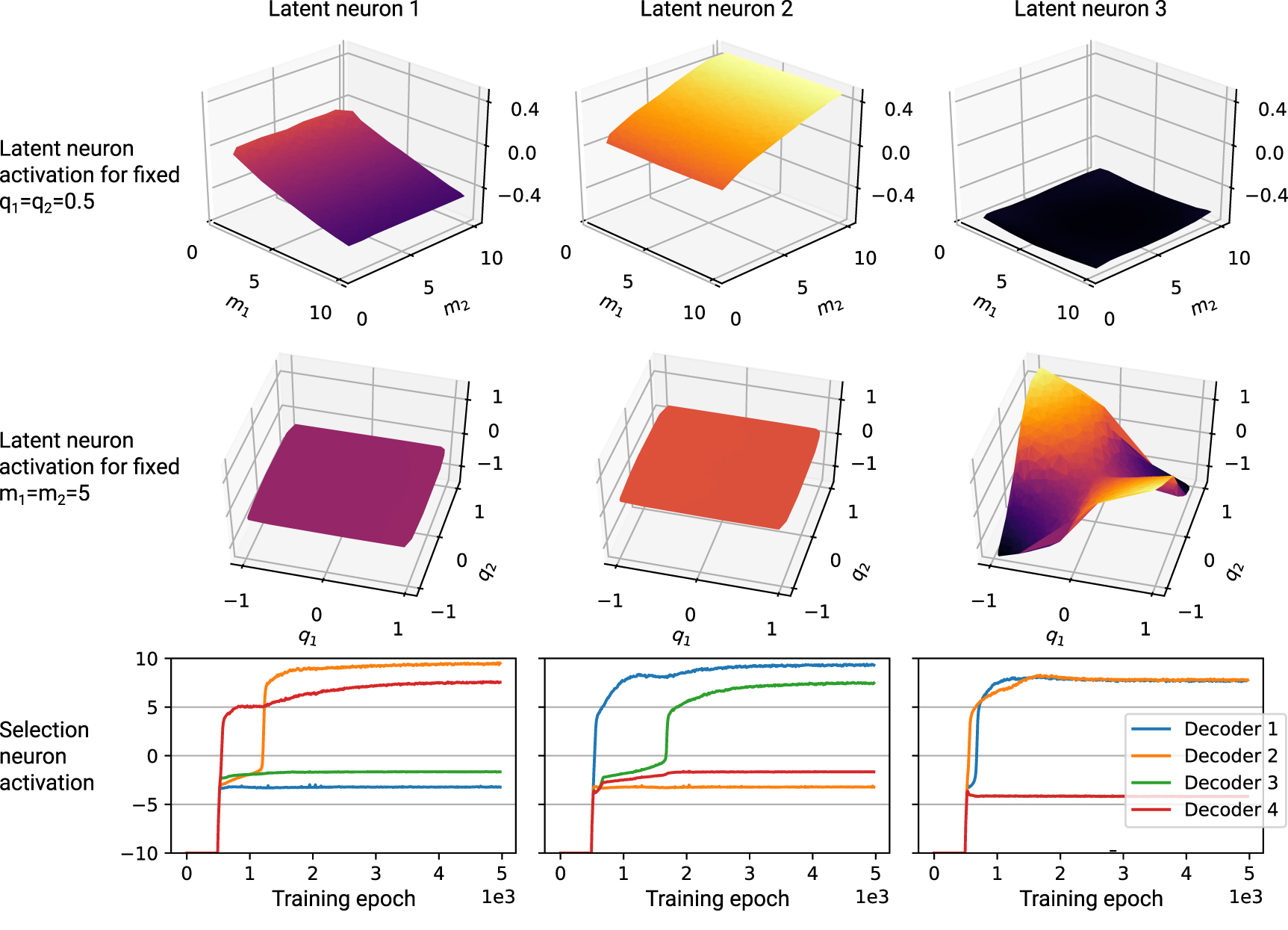
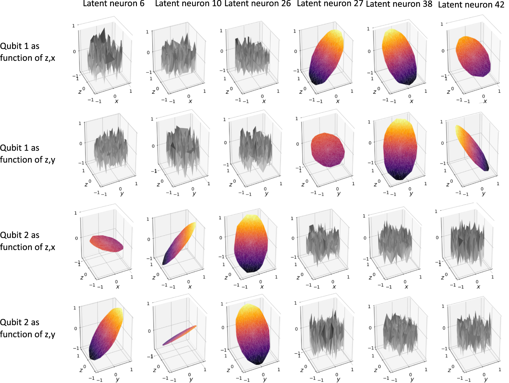