


Abstract
Force-free electrodynamics (FFE) describes magnetically dominated relativistic plasma via non-linear equations for the electromagnetic field alone. Such plasma is thought to play a key role in the physics of pulsars and active black holes. Despite its simple covariant formulation, FFE has primarily been studied in 3+1 frameworks, where spacetime is split into space and time. In this paper, we systematically develop the theory of force-free magnetospheres taking a spacetime perspective. Using a suite of spacetime tools and techniques (notably exterior calculus), we cover (1) the basics of the theory, (2) exact solutions that demonstrate the extraction and transport of the rotational energy of a compact object (in the case of a black hole, the Blandford–Znajek mechanism), (3) the behaviour of current sheets, (4) the general theory of stationary, axisymmetric magnetospheres, and (5) general properties of pulsar and black hole magnetospheres. We thereby synthesize, clarify, and generalize known aspects of the physics of force-free magnetospheres, while also introducing several new results.
1 INTRODUCTION
Soon after the discovery of pulsars (Hewish et al. 1968) it became clear that they must be rapidly rotating, highly magnetized neutron stars (Gold 1968; Pacini 1968) whose magnetosphere is filled with plasma (Goldreich & Julian 1969). The plasma mass density is many orders of magnitude lower than the electromagnetic field energy density, so one may neglect the plasma four-momentum and set the Lorentz four-force density to zero. The resulting autonomous dynamics for the electromagnetic field, known as force-free electrodynamics (FFE), forms a foundation for studies of the pulsar magnetosphere.
Quasars were discovered several years before pulsars (Schmidt 1963), and while supermassive black holes were soon suspected as the energy source, more than a decade passed before the discovery of a viable mechanism for extracting the energy. The breakthrough was the seminal work of Blandford & Znajek (1977, BZ), who argued that black holes immersed in magnetic fields could have a force-free plasma. BZ showed that the presence of plasma enables a magnetic Penrose process in which even stationary fields can efficiently extract energy from a spinning black hole.
Despite this important progress, little further was done on the subject for several years. MacDonald & Thorne (1982) diagnosed the difficulty as a problem of language. In addition to significantly extending the theory, they recast the work of BZ in a 3 + 1 decomposition designed to render the equations and concepts more familiar to astrophysicists. The efficacy of their cure is well supported by the significant progress on the problem that has been made since then, nearly all of it using the 3 + 1 approach.
But even the best medicines can have side effects. From the relativist's point of view, the use of 3 + 1 methods obscures intrinsic structures and creates unnecessary complications by introducing artificial ones. For a subject in which curved spacetime and highly relativistic phenomena play central roles, one might expect that the impressive arsenal of spacetime techniques developed over the last century could be profitably exploited. However, very few general relativity theorists have become involved, and little work of this nature has been pursued. It may be that the unfamiliar language and phenomena of plasma physics, together with their casting in 3 + 1 language, have made the subject largely inaccessible to relativists.
The beginnings of the field were in fact rather relativistic in flavour, with Znajek's (1977) use of a null tetrad formalism and BZ's tensor component calculations. Since then however there has been little use of spacetime techniques on black hole and pulsar force-free magnetospheres, notable exceptions being the work of Carter (1979) and Uchida (1997a,b,c,d, 1998). Our own involvement began recently when we noticed that some apparently disparate exact solutions shared the property of having four-current along a geodesic, shear-free null congruence (Brennan, Gralla & Jacobson 2013). We made a null current ansatz and immediately found a large class of non-stationary, non-axisymmetric exact solutions in the Kerr spacetime, which can also be used in flat spacetime in modelling pulsar magnetospheres. This rapid progress suggested to us that translation of magnetospheric physics into spacetime language may be more than a matter of words, and that a geometrical perspective on FFE could lead to powerful insights and significant new results.
This paper has a number of distinct purposes. One is to present the theory of force-free magnetospheres with a spacetime perspective from the ground up. In this way we hope both to introduce relativists to the subject and to introduce plasma astrophysicists to potentially powerful new techniques. We focus on intrinsic properties, avoiding the introduction of arbitrary structures – such as a time function or a reference frame – that have no intrinsic relation to either the spacetime geometry or the particular electromagnetic field being discussed. The other purposes of our paper are to present new insights, techniques, and results, as well as the convenient methods of exterior calculus we have made use of.
The paper is organized into nine sections and five appendices:
1. Introduction
2. Astrophysical setting
3. Force-free electrodynamics
4. Poynting flux solutions
5. Monopole magnetospheres
6. Current sheets and split monopoles
7. Stationary, axisymmetric magnetospheres
8. Pulsar magnetosphere
9. Black hole magnetosphere
A. Differential forms
B. Poynting flux examples
C. Kerr metric
D. Euler potentials with symmetry
E. Conserved Noether current associated with a symmetry.
We now provide a detailed description of the contents of each section.
In Section 2, we sketch the relevant astrophysical settings and discuss the basic reasoning that accounts for the validity of the force-free approximation. We then present the basic features and mathematical structure of FFE and degenerate electromagnetic fields (Section 3). This section is primarily a review and synthesis of previous research, focusing on the spacetime approaches of Carter and especially Uchida, who formulated the theory in terms of two scalar Euler potentials. We have found that the use of differential forms (with wedge product and exterior derivative) together with Euler potentials provides an elegant and computationally efficient method to handle the mathematics, and we focus on this approach throughout the paper. Appendix A covers the properties of differential forms needed in the paper. We emphasize the geometrical role of certain timelike 2-surfaces that, for degenerate magnetically dominated fields, extend the notion of field line to a spacetime object. These are called ‘flux surfaces’ in the literature, but we adopt here the more suggestive name ‘field sheets’. In particular, we observe that the induced metric on these sheets governs the dynamics for particles and Alfvén waves moving in the magnetosphere, and explain how field sheet Killing fields give rise to conserved quantities. We also note that the field equations of FFE amount to the conservation of two ‘Euler currents’, which have not been explicitly discussed before.
Section 4 is devoted to presenting several exact solutions to FFE involving outgoing electromagnetic energy flux (Poynting flux) in flat, Schwarzschild, and Kerr spacetimes. These include a solution in Kerr recently found by Menon & Dermer (2007), a time-dependent and non-axisymmetric generalization of that (Brennan et al. 2013), as well as a solution sourced from an arbitrary accelerated world line in flat spacetime (Brennan & Gralla 2014). We showcase the remarkably simple expression of these solutions in the language of differential forms, as well as the efficient computational techniques we can use to check that they are force free. The solutions illustrate how force-free fields can transport energy via Poynting flux in ways that are unfamiliar in (but not completely absent from) ordinary electrodynamics. Appendix B is devoted to examples that further develop insight into the physical nature of this energy transport.
Turning next to the physics of magnetospheres, Section 5 builds on the Poynting flux solutions to present several exact solution models with a monopolar central rotating source. (The more realistic case of a split monopole is deferred for clarity to the next section.) We begin with a discussion of the classic Michel solution, which illustrates the basic mechanism of electromagnetic extraction and transport of the rotational energy of a conducting magnetized star. We obtain this solution as a superposition of a monopole and an outgoing Poynting flux solution satisfying the perfect conductor boundary condition, and use it to illustrate the nature of field sheet geometry. We next show how our time-dependent generalizations can be used to model dynamical pulsar magnetospheres. In particular, we debut the ‘whirling monopole’, which is the exact monopolar magnetosphere of a conducting star undergoing arbitrary time-dependent rigid body motion with a fixed centre. Finally, we discuss the monopolar approximate solution of BZ for a rotating black hole. We obtain their solution to first order in the spin by promoting the Michel solution to Kerr in a simple way. The result is an exceptionally simple expression for the BZ field in terms of differential forms, from which its force-free nature as well as basic properties (such as its ‘rotation frequency’ of one half the horizon frequency) are easily seen.
In Section 6, we discuss the role of current sheets in force-free magnetospheres and provide a simple invariant criterion for the shape and time evolution of a current sheet across which the electromagnetic field flips sign. We use this criterion to efficiently reproduce the standard aligned and inclined split-monopole solutions and discuss generalizations, such as a glitching split-monopole pulsar. We also discuss a more general, reflection split construction in which the magnetic field has a component normal to the current sheet.
Section 7 is devoted to the general theory of stationary, axisymmetric, force-free magnetospheres in stationary, axisymmetric spacetimes. We make extensive use of the natural 2 + 2 decomposition into ‘toroidal’ submanifolds spanned by the angular and time-translation Killing vectors and the orthogonal ‘poloidal’ submanifolds. The Uchida (1997b) method of determining the general form of Euler potentials for fields with symmetry is presented using differential forms in Appendix D. We explain how and why the field is characterized by three quantities: the ‘magnetic flux function’ ψ, the ‘angular velocity of field lines’ ΩF(ψ), and the ‘polar current’ I(ψ), derive the general force-free ‘stream equation’ relating these quantities, and discuss approaches to solving it. Expressions for the energy and angular momentum flux are derived, using the corresponding Noether current 3-forms whose derivation is given in Appendix E. We explain how the ‘light surfaces’ (where the field rotation speed is that of light) are causal horizons for particles and Alfvén waves, and derive the relationship between the particle and angular momentum flow directions. We discuss general restrictions on the topology of poloidal field lines, presenting a new result that smooth closed loops cannot occur and clarifying the circumstances under which field lines cannot cross a light surface twice. Finally, we present the stream equation for the special case where there is no poloidal magnetic field, which has been largely overlooked in previous work.
Section 8 discusses basic properties of the pulsar magnetosphere in the case of aligned rotational and magnetic axes, using the stationary, axisymmetric formalism of the previous section. We discuss the corotation of the field lines with the star as well as the dichotomy between closed field lines that intersect the star twice and open field lines that proceed from the star to infinity. We clarify the precise circumstances under which closed field lines must remain within the light cylinder, and discuss other circumstances in which they may extend outside.
Section 9 addresses black hole magnetospheres, focusing on stationary, axisymmetric fields in the Kerr geometry. We derive the so-called Znajek horizon regularity condition and identify an additional condition required for regularity in the extremal case. We discuss the status of energy extraction as a Penrose process and discuss the nature of the two light surfaces. Finally, we present the ‘no-ingrown-hair’ theorem of MacDonald & Thorne (1982), showing that a black hole cannot have a force-free zone of closed poloidal field lines. We discuss the types of closed field lines that can in fact occur.
We adopt the spacetime signature ( −, +, +, +), choose units with the speed of light c = 1 and Newton's constant G = 1, and use Latin letters a, b, c, … for abstract tensor indices (there is no use of coordinate indices in the paper). For Maxwell's equations, we use Heaviside–Lorentz units.
2 ASTROPHYSICAL SETTING
Force-free plasmas exist naturally in pulsar magnetospheres, and possibly in several other astrophysical systems. Goldreich & Julian (1969) pointed out that the rotation of a magnetized conducting star in vacuum induces an electric field, with the Lorentz scalar |$\boldsymbol {E} \cdot \boldsymbol {B}$| non-zero outside the star. Undeflected acceleration of charges along the direction of the magnetic field will thus occur. For typical pulsar parameters, the electromagnetic force is large enough to overwhelm gravitational force and strip charged particles off the star. Even if strong material forces retain the particles, the large |$\boldsymbol {E} \cdot \boldsymbol {B}$| outside the star will create particles in another way (Ruderman & Sutherland 1975): any stray charged particle will be accelerated to high energy along curved magnetic field lines, leading to curvature radiation and a cascade of electron–positron pair production. These mechanisms act to fill the pulsar magnetosphere with plasma.
To estimate the density of plasma, note that produced charges act to screen the component of |$\boldsymbol {E}$| along |$\boldsymbol {B}$|, eventually shutting off production when |$\boldsymbol {E} \cdot \boldsymbol {B}$| becomes small enough. The number of particles created should thus roughly agree with the minimum amount required to ensure |$\boldsymbol {E} \cdot \boldsymbol {B}=0$|. If the particles corotate with the star, the required charge density is the so-called Goldreich–Julian charge density ρ ∝ ΩB, where Ω is the stellar rotation frequency. The minimum associated particle density occurs for complete charge separation (one sign of charge only at each point), which for typical pulsar parameters corresponds to a plasma rest mass density that is 16–19 orders of magnitude (for protons or electrons, respectively) smaller than the electromagnetic field energy. Even if particle production mechanisms significantly overshoot this density, the criterion for the force-free description is easily satisfied.1 Detailed calculations support these simple arguments, finding an overshoot of a few orders of magnitude (e.g. Beskin 2010).
Force-free models of the pulsar magnetosphere provide a foundation on which studies of pulsar emission processes may be based. Models of pulsed emission generally involve particles or plasma instabilities streaming outwards along the magnetic field lines of the magnetosphere (e.g. Beskin 2010). Pulsed emission is observed in radio, optical, X-ray, and gamma-ray, with some pulsars active only in a subset of these bands, and with a variety of pulse profiles. The challenge of modelling these complex features remains an active field of research.
The force-free model has also been applied to black holes, beginning with the work of BZ. Following the observation of Wald (1974) that immersing a spinning black hole in a magnetic field gives rise to electric fields with non-zero |$\boldsymbol {E} \cdot \boldsymbol {B}$|, BZ argued that a pair-production mechanism could also operate to produce a force-free magnetosphere near a spinning black hole with a magnetized accretion disc. If the whole system is simulated using magnetohydrodynamics (MHD; e.g. McKinney, Tchekhovskoy & Blandford 2012 and references therein), it is generally found that the plasma density is very low away from the disc (and especially in any jet region), so that the dynamics there is effectively force free. Finally, the last few years has seen work on force-free magnetospheres of binary black hole and neutron star systems (e.g. Palenzuela, Lehner & Liebling 2010; Alic et al. 2012; Palenzuela et al. 2013; Paschalidis, Etienne & Shapiro 2013), motivated in part by the possibility of observing electromagnetic counterparts to gravitational-wave observations of binary inspiral. These simulations have shown energy extraction and jet-like features, even in the case of non-spinning (but moving) black holes.
3 FORCE-FREE ELECTRODYNAMICS
In this section, we introduce the essential properties of FFE in an arbitrary curved spacetime background and its description in the language of differential forms.
3.1 Determinism
There is no a priori reason to expect that the condition B2 > E2 is preserved under time evolution. In fact, it is seen numerically that the condition is not preserved. When the condition is violated, some other physics must determine the evolution, which is modelled via various prescriptions in numerical codes. It is generally found that violation occurs only in regions that are stable under the associated prescriptions, and that these regions tend to be compressed and of high current density: they are the current sheets discussed below in Section 6.
3.2 Degenerate electromagnetic fields
In this subsection, we discuss electromagnetic fields satisfying F[abFcd] = 0 (equivalently |$\boldsymbol {E}\cdot \boldsymbol {B}=0$| in flat spacetime), which are called degenerate. All force-free fields are degenerate, but degeneracy can occur more generally, as explained below.
3.2.1 Field tensor
For a magnetically dominated field, the α–β plane is thus spacelike and the kernel, which is orthogonal to α and β, is timelike. There is a one-parameter family of four-velocities Ua lying in this timelike kernel, each of which defines a Lorentz frame in which the electric field vanishes (equation 13). The orthogonal projection of a preferred frame ta into the kernel of F selects one of these, |$U_t^a$|, whose velocity relative to ta is known as the drift velocity. This relative velocity is the minimum for all Ua in the kernel of F, and is given by |$\boldsymbol E\times \boldsymbol B/B^2$| in the frame ta.
For a field with E2 = B2, either α or β must be null, so the α–β plane is null and so is the kernel (with the same null direction). For an electrically dominated field, the α–β plane is timelike, so the kernel is spacelike, and there is always a Lorentz frame in which the magnetic field vanishes (since the kernel of *F is timelike).
3.2.2 Stress tensor
In the magnetic case and in a 3 + 1 decomposition, equation (15) may be interpreted in terms of the standard concepts magnetic pressure and magnetic tension. Choose any frame in which there is no electric field i.e. any unit timelike Ua in the kernel of F. Let sa be the unit orthogonal spacelike vector in the kernel. The magnetic field in this frame is directed along sa, and we denote its magnitude by B. If γab is the spatial metric orthogonal to Ua, then the stress tensor (equation 15) may be written |$T_{ab} = \frac{1}{2} B^2 (U_a U_b + \gamma _{ab} - 2 s_a s_b)$|. From each term, respectively, we identify the energy density of |$\frac{1}{2}B^2$|, an isotropic magnetic pressure of |$\frac{1}{2}B^2$|, and a magnetic tension of B2 along the magnetic field lines.
3.2.3 Field sheets
When a degenerate field Fab satisfies the Maxwell equation ∇[cFab] = 0 (3), the kernels of Fab are integrable, i.e. tangent to two-dimensional submanifolds. (A proof of this will be given in the next subsection.) In the magnetic case (F2 > 0), these submanifolds are timelike, and their intersection with a spacelike hypersurface gives the magnetic field lines defined by the observers orthogonal to the hypersurface.3 Each submanifold can thus be thought of as the spacetime evolution of a field line, which we will call a field sheet.4 While the field lines depend on the arbitrary choice of spacelike hypersurface or observers, the field sheets are an intrinsic aspect of the degenerate structure of the field. The force-free condition (2) amounts to the statement that the current four-vector ja is tangent to the field sheets. This generalizes to dynamical fields in curved spacetime the statement that, in a force-free plasma with zero electric field in flat spacetime, the current is tangent to the magnetic field lines.
The field sheets can be used to understand and describe particle and wave motion in the underlying plasma in a manner that does not require choosing an arbitrary frame. In that application the field sheet metric, induced by the spacetime metric, plays a central role. We now discuss two examples of this viewpoint: the propagation of charged particles and Alfvén waves.
In a collisionless plasma, viewed (locally) in a frame with zero electric field, a charged particle will spiral around a magnetic field line, executing cyclotron motion while the centre of the transverse circular orbit is ‘guided’ along the field line. Ignoring the cyclotron motion and the drift away from the field line, the particle is thus ‘stuck’ on the field line (e.g. Northrop & Teller 1960). The manifestly frame-invariant version of this statement is that the particle's world line is stuck on the field sheet. That is, its possible motions are the timelike trajectories on the sheet.
When one can furthermore neglect radiation reaction from ‘curvature radiation’ due to the bending of the field sheet, then the motion of the particle is in fact geodesic on the field sheet. This follows simply from the fact that the Lorentz force qFabUb vanishes for a four-velocity Ua tangent to the sheet. This viewpoint makes it easy to exploit symmetries. For example, in a stationary, axisymmetric magnetosphere, each field sheet will have a helical symmetry under a combined time-translation and rotation. The field sheet particle motion, being one-dimensional, will thus be integrable using the associated conserved quantity (see Section 7.2.6).
Field sheet geometry also governs the propagation of Alfvén waves, which are transverse oscillations of the magnetic field lines embedded in a plasma (Alfvén 1942). In a force-free plasma, these are characterized by a wave four-vector whose pullback to the field sheet is null with respect to the field sheet metric (Uchida 1997d), which implies that their group four-velocity is null and tangent to the field sheet. Thus wavepackets propagate at the speed of light along the field sheets.
3.2.4 Degenerate fields and differential forms
The mathematical language of differential forms is ideally suited to working with degenerate fields, and we shall make extensive use of it in this paper. The basic properties of differential forms are summarized in Appendix A, to which we refer for all definitions. One of the reasons it is so convenient is that electromagnetism in general, and especially when fields are degenerate, has a rich differential and algebraic structure that is in fact independent of the spacetime metric. By using the (metric-independent) exterior derivative, and (metric-independent) wedge products rather than covariant derivatives and inner products, we avoid unnecessary appearance of the metric and thus keep the formalism as close as possible to the structure inherent in the field itself. The metric does of course play a role, but for the most part we can sequester that in the Hodge duality operator (which is especially simple to work with in stationary axisymmetric spacetimes).
To prove that the field sheets exist, one can invoke a version of the Frobenius theorem: it follows from dF = 0 and F = α ∧ β, together with the antiderivation property of d and antisymmetry of ∧, that dα ∧ α ∧ β = dβ ∧ α ∧ β = 0. This guarantees complete integrability of the Pfaff system α = β = 0 (Choquet-Bruhat & Dewitt-Morette 1982), which means that the vectors annihilating both α and β are tangent to submanifolds. A more intuitive argument for integrability will be given in the next subsection.
3.2.5 Frozen flux theorem
To prove the theorem, consider a loop flowed along U to create a timelike tube, and form a closed 2-surface by capping the ends of the tube with topological discs bounded by the initial and final loops. The integral of F over any closed 2-surface vanishes since dF = 0. The difference of the fluxes through the initial and final caps is therefore equal to the integral of F on the tube wall, which vanishes because the vector U that annihilates F (equation 19) is tangent to the wall. Using the language of differential forms, Alfvén's theorem is thus recovered immediately, with no calculation, in an arbitrary curved spacetime. It is interesting to contrast the simplicity of this completely general derivation with the usual one using electric and magnetic fields in flat spacetime.
The frozen flux theorem is closely related to the integrability property that implies the existence of the field sheets. In fact we can use it to give a simple proof of integrability as follows. Recall that if F is degenerate, there is a two-dimensional space of vectors annihilating F at each point. To prove these are surface forming, let u be any vector field such that u · F = 0 everywhere. As above, Cartan's magic formula implies |${\cal L}_u F = 0$|. Now choose a second vector field b such that b · F = 0 on one 3-surface transverse to the flow of u, and extend b along the flow by requiring |${\cal L}_u b = 0$|, which implies that u and b are surface forming. The Leibniz rule for Lie derivatives implies |${\cal L}_u (b\cdot F)=0$|, so also b · F = 0 everywhere. The integral surfaces of u and b are therefore the field sheets.
3.2.6 Euler potentials
The Euler potentials capture the freedom in a closed, simple 2-form, hence in any degenerate electromagnetic field. Rather than the four components of a (co)vector potential, there are just two scalar fields. Even so, the potentials are not uniquely determined. F defines an ‘area element’ on the field sheets, which is preserved under any replacement |$(\phi _1,\phi _2)\rightarrow (\phi _1^{\prime }(\phi _1,\phi _2), \phi _2^{\prime }(\phi _1,\phi _2))$| with unit Jacobian determinant. This is a field redefinition, not a dynamical gauge freedom. In fact, the second time derivatives of both potentials are determined at each point by their value and first derivatives (Uchida 1997a).
3.3 Euler-potential formulation of FFE
Since all force-free fields are degenerate, we may formulate FFE as a theory of two scalar fields by plugging the Euler-potential form of a degenerate field strength (equation 22) in to the force-free condition (2). Rather than developing this technique in tensor language, we will instead discuss the differential forms version, which we find very useful in calculations. We also discuss an action principle for the equations.
3.3.1 Force-free condition and Euler currents
3.3.2 Action
The action is a scalar, so the stress–energy tensor is conserved when the equations of motion are satisfied. This is to be expected, since our starting point was the force-free condition which implies that the field transfers no energy or momentum to the charges. Moreover, the dynamics share the symmetries possessed by the * operator on 2-forms, namely symmetries and Weyl rescalings of the metric. This implies, for instance, that in a stationary axisymmetric spacetime there are conserved Killing energy and axial angular momentum currents, and that FFE shares with vacuum electrodynamics the property of depending only on the conformal structure of the spacetime. The potentials can also be restricted by a symmetry ansatz before variation, to directly obtain the equations governing the symmetric solutions.
3.3.3 Complex Euler potential
Finally, it seems worth noting that the two Euler potentials can be combined into one complex potential |$\phi = (\phi _1+i\phi _2)/\sqrt{2}$|. Then the field 2-form is given by |$F=i\, {{d}}\phi \wedge {{d}}\bar{\phi }$|, the force-free field equations correspond to the single complex equation dϕ ∧ d * F = 0, and the action is |${\textstyle {\frac{1}{2}}}\int {{d}}\phi \wedge {{d}}\bar{\phi }\wedge \ast ({{d}}\phi \wedge {{d}}\bar{\phi })$|. Whether this complex formulation is useful remains to be seen.
4 POYNTING FLUX SOLUTIONS
In this section, we recover and discuss a number of exact solutions to the force-free field equations (25) using the method of exterior calculus. In addition to introducing some important properties of force-free physics, we hope that this section will serve as a tutorial on computing with differential forms, for readers unfamiliar with that approach. The most unfamiliar element is perhaps the use of the Hodge dual in place of the metric. In Appendix A2, we review this operator and develop some computational techniques. With the aid of these techniques, computations using forms can be remarkably simple, as we demonstrate below. We begin by discussing the magnetic monopole, then cover solutions describing purely outgoing (or ingoing) Poynting flux, and finally superpose these to obtain the general solution used to construct monopole magnetospheres in the following section.
4.1 Vacuum monopole
The 2-form (equation 29) is simple, i.e. the monopole field is degenerate. In particular, this implies that it can be expressed in terms of Euler potentials, which can be taken as ϕ1 = −qcos θ and ϕ2 = φ. Note that the discontinuity of φ at 2π means that the Euler potential is not globally smooth. This presents no problem; moreover, were it not for this discontinuity, the field would be an ‘exact form’ dAmon, with Amon = qφ d(cos θ), so the total magnetic flux through the closed surface of the two-sphere would necessarily vanish.8
4.2 Outgoing Poynting flux
The energy flow in the field (30) is unlike ordinary electromagnetic radiation in that the flux persists for stationary fields, i.e. energy is carried away even if ζ is independent of u. In this case, the solution has more the character of a flow than a wave, and such flows are sometimes called ‘electromagnetic winds’ or ‘Poynting winds’. For vacuum fields, this situation is impossible with isolated sources, but it does occur in waveguides and in planar symmetry. In fact, these scenarios admit vacuum solutions that are highly analogous to equation (30). In Appendix B, we explore these examples as context for understanding the outgoing flux solution.
By itself, the outgoing flux solution is unphysical, since it describes energy emerging from the origin of coordinates in flat spacetime (where the solution is singular), or from the past horizon on the analytic extension of the Schwarzschild spacetime.10 Additionally, as a null field, it lies on the threshold of the electrically dominated regime, and thus might be unstable to non-force-free processes. However, as described below, the solution is physically realized as part of magnetically dominated field configurations associated with a rotating star or black hole, which sources the outflow of energy.
The current J ∼ dθ ∧ dφ ∧ du of the outgoing flux solution is a null 3-form. The dual of such a form is proportional to the null factor du (see Appendix A2.4), so we have ja ∼ (du)a. That is, the current four-vector is null and radial. If the charges all have the same sign, they must be moving at the speed of light, but a null current can also be composed of charges of opposite sign moving such that the net charge density is equal to the magnitude of the net three-current in any Lorentz frame. The force-free equations are sensitive only to the net charge-current.
It is rather curious that a purely outgoing solution exists on a Schwarzschild background. One would expect that waves would backscatter from the effective potential caused by the spacetime curvature. The existence of non-scattering solutions like these was discovered by Robinson (1961). He showed that, associated with any shear-free null geodesic congruence, there is a family of null, non-scattering vacuum solutions to Maxwell's equations. For the radial outgoing null congruence in the Schwarzschild spacetime, the Robinson solutions are exactly the fields (equation 30) with Δ2ζ = 0. These are in some sense illusory solutions, since they are not globally regular on the sphere. However, they are resurrected as bona fide, regular solutions in the force-free context.
4.3 Outgoing flux from an arbitrary world line
In flat spacetime, the energy flux of equation (30) emerges from the origin of coordinates, which may be identified with a stationary world line. In fact, the solution generalizes readily to an arbitrary timelike world line, where u is taken to be the associated retarded time. That is, on the future light cone of any point p on the world line, u is the proper time at p. Then precisely the same expression (30) is a solution, if (r, θ, φ) are any coordinates such that dθ and dφ are orthogonal to du, for example, global inertial spherical angles. This follows from the same computation used to check that equation (30) is a solution. This solution was first found in Brennan & Gralla (2014) using the Newman–Penrose formalism.
4.4 Outgoing flux in Kerr
We next present the generalization of the outgoing flux solution (30) to a rotating black hole background, i.e. the Kerr spacetime. The stationary axisymmetric version of this solution was found by Menon & Dermer (2007, 2011), and it was generalized to the non-stationary, non-axisymmetric case in Brennan et al. (2013) using the Newman–Penrose formalism. Here we recover that generalized solution using the exterior calculus.
It is simple to describe the solution using outgoing Kerr coordinates |$(u, \bar{\varphi }, \theta , r)$|, which are defined in Appendix C. A first guess would be that the field (30) is a solution, with the substitution |$\varphi \rightarrow \bar{\varphi }$|. However, that is not correct, because in Kerr the 1-form du is timelike rather than null, and the null property of du played a critical role in establishing that equation (30) is a solution in Schwarzschild. To motivate a modification, and to proceed with the calculations, we need the following properties of the Kerr metric in these coordinates (see Appendix C): (i) the 1-form |${{d}}u - a\sin ^2\theta \, {{d}}\bar{\varphi }$| is null and orthogonal to the 1-forms du, |${{d}}\bar{\varphi }$|, and dθ; and (ii) dθ and |${{d}}\bar{\varphi }$| are orthogonal to each other, and the ratio of their norms is sin θ.
Note that, like in the Schwarzschild case, this solution has the remarkable property that the radiation has no backscattering. This is again directly linked to Robinson's theorem: the congruence tangent to the null vector obtained by contraction of |${{d}}u - a\sin ^2\theta \, {{d}}\bar{\varphi }$| with the inverse metric is geodesic and shear free. [It is the outgoing principal null congruence of the Kerr metric (e.g. Poisson 2004).] And again, there is no globally regular vacuum solution of this type, but in the presence of non-zero current there are regular force-free solutions. These solutions were first found by assuming that the current is along the principal null congruence (Brennan et al. 2013). That analysis also shows that there are no other solutions with such a current.
4.5 Ingoing flux
By taking the time-reverse12 of the outgoing flux solution, one obtains an ingoing flux solution. This solution represents energy emerging from a distant region and converging on the origin of flat spacetime, or entering the horizon of a black hole. In the black hole case, the ingoing flux is regular at the future horizon and totally absorbed by the black hole, with no backscattering.
4.6 Superposed monopole and flux
Unfortunately, this simple construction does not generalize to the Kerr background. Although exact monopole13 and outgoing flux solutions on Kerr are known, the monopole field exerts a force on the null current. [This obstruction is a special case of a general theorem: a solution with current along a null geodesic twisting congruence cannot be magnetically dominated (Brennan et al. 2013).]
An interesting generalization applies however to a monopole moving along an arbitrary world line in Minkowski space: the dual of the Lienard–Wiechert vacuum field can be superposed with the outgoing flux solution described in Section 4.3 (Brennan & Gralla 2014). This yields a magnetically dominated solution, in which normal radiation (in the dual Lienard–Wiechert field) coexists with current-supported Poynting flux.
5 MONOPOLE MAGNETOSPHERES
In this section, we apply the solutions discussed in the previous section to model magnetospheres external to rotating stars and black holes with monopole charge. These models present basic physical properties of force-free magnetospheres in a simple setting, most importantly the conversion of rotational kinetic energy to Poynting flux. Using the same solutions, a closer approximation to real magnetospheres is obtained by ‘splitting’ the monopole, as discussed in Section 6.
5.1 Rotating monopole (Michel solution)
The current 3-form for the Michel solution is given by equation (33), which evaluates to J = −qΩsin 2θ dθ ∧ dφ ∧ du. Equivalently, the current four-vector is equal to the radial null vector ja = −2qΩ(cos θ/r2)(∂r)a.14 In the northern hemisphere, this is a radial ingoing three-current and a negative charge density of the same magnitude as the three-current, while in the southern hemisphere, it is a radial outgoing three-current and a positive charge density.
The Michel monopole illustrates a key physical effect of pulsar physics: a rotating, magnetized conductor generates an outgoing energy flux, even when stationary.
5.1.1 Field sheet geometry of the Michel monopole
The field of a monopole rotating in vacuum would of course be identical to that of a static monopole, but the Michel solution is in a certain sense ‘really rotating’. The structure of this field can be elucidated via the geometry of its field sheets. The Euler potentials can be taken as ϕ1 = −qcos θ and ϕ2 = φ − Ω(t − r), so the field sheets are the surfaces where θ and φ − Ω(t − r) are constant. Lab frame field lines (intersections of the sheets with constant t planes) form Archimedean spirals in the equatorial plane, and conical helices for other values of θ (see Fig. 2). At successive times t and t + Δt, these lines are rotated relative to each other by an angle ΩΔt, so one may think of the lines as rotating with angular velocity Ω. They are also related by r → r + Δt, however, so one may equivalently think of them as expanding outwards at the speed of light. The field sheet is independent of which way one thinks of field line evolution (and also of the choice of frame used to define field lines). A spacetime plot of two equatorial field sheets is given in Fig. 1.
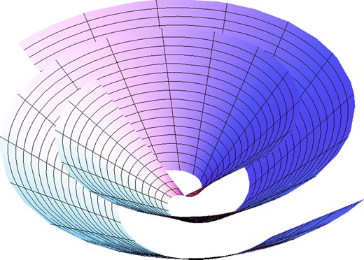
Two equatorial field sheets of the Michel monopole.
The field sheet metric is obtained by imposing the conditions dθ = 0 and dφ = Ω du in the Minkowski metric, which yields ds2 = −(1 − r2Ω2sin 2θ)du2 − 2du dr. Amusingly, this is nothing but 1+1 dimensional de Sitter spacetime in ‘Eddington–Finkelstein’ form. The de Sitter horizon corresponds to the light cylinder rsin θ = 1/Ω where a corotating observer would move with the velocity of light. The ‘Hubble constant’ is Ωsin θ, which is also the surface gravity of the horizon. This Killing horizon interpretation of the light cylinder extends to general stationary axisymmetric magnetospheres, as we discuss in Section 7.2.5.
5.1.2 Differential rotation
Equation (41) remains a solution when Ω is promoted to an arbitrary function of θ. This corresponds to a conducting star that rotates at latitude-dependent speed. This generalization of the Michel monopole was first noted by BZ (see equation 6.4 therein). It corresponds to choosing ζ = −q∫sin θ Ω(θ)dθ in the superposed solution (38). On account of the θ-dependence of ζ, the power radiated is modified from the Michel form (42).
5.1.3 Variable rotation rate
Equation (41) remains a solution when Ω is promoted to an arbitrary function of u, or more generally of u and θ. This corresponds to a conducting star whose rotational speed changes with time. The changes propagate outwards into the magnetosphere at the speed of light. This generalization of the Michel monopole was first noted by Lyutikov (2011). It corresponds to choosing ζ = −q∫sin θ Ω(θ, u) dθ in the superposed solution (38). The flux at each retarded time u is given by the instantaneous value of the associated stationary solution.
5.2 Whirling monopole
5.3 Black hole monopole (BZ solution)
As described in Section 4.6, the procedure of superposing monopole and outgoing flux solutions fails to produce a solution in Kerr. However, long ago BZ found a perturbative monopolar solution describing a stationary, axisymmetric outgoing flux of energy from a Kerr black hole to second order in the black hole spin parameter a. This solution may be recovered to first order in a simply by promoting the Michel monopole solution to Kerr, as we now explain. Recovering the second-order perturbations is also straightforward, though more involved. We focus on the first-order piece, which provides the leading outgoing energy flux.
Since there is no current in the monopole solution, the second factor in the force-free conditions (24) vanishes at O(a0); hence, in the O(a) equation, the first factor (α or β) may be taken to be the zeroth-order parts d(−qcos θ) and dφ. Thus up through O(a), the force-free conditions amount to dθ ∧ J = dφ ∧ J = 0, i.e. the statement that both dθ and dφ are factors in the current 3-form d * F. The O(a) terms in d * F have two origins: the Ω term in equation (44) and the O(a) part of the action of * on the zeroth-order (monopole) solution. The contribution of the Ω term to the current is Ωd * (sin θ dθ ∧ du) = Ωd(sin 2θ dφ ∧ du) ∼ dθ ∧ dφ ∧ du, which has both dθ and dφ as factors. The O(a) part of *(dθ ∧ dφ)μν = 2ϵθφrtgr[μgν]t comes from gφt, the only O(a) part of the Kerr metric in BL coordinates. Since |$g_{r\mu }\propto \delta _\mu ^r$|, this O(a) contribution has the form C(r, θ)dr ∧ dφ for some function C. It therefore contributes to the current d * F, a 3-form ∼dθ ∧ dr ∧ dφ, which also has both dθ and dφ as factors. Hence, the force-free condition is satisfied at O(a).
Rotating stars
To first order in the spin, the exterior metric of a rotating star is given by the Kerr metric linearized in a (Hartle & Thorne 1968). We may thus also use equation (44) to model stellar magnetospheres, including the leading gravitational effects of spin. As in the previous subsection, imposition of conducting boundary conditions at the star will fix Ω to equal the rotational velocity of the star. It is interesting to compare this with the black hole case (46), where there is an additional factor of one-half. As will be seen in Section 9, the energy flux from any axisymmetric black hole magnetosphere would vanish if the angular velocity of the field were equal to that of the black hole horizon.
6 CURRENT SHEETS AND SPLIT MONOPOLES
We have seen that the superposition of monopole and outgoing radiation solutions provides a simple analytic solution describing energy flux from rotating stars and black holes. The catch, of course, is that real stars and black holes do not have monopoles inside them! A cheap trick for addressing this last point is to artificially split the monopole in two or more parts, reversing the sign of the monopole charge (and perhaps also rescaling the charge) when passing from one region to the next. A crude model of a dipole can be constructed in this way, for example, while still using only the monopole solution. However, this splitting of the field has a dramatic consequence that must be confronted: since the field changes direction discontinuously across the splitting surface, Maxwell's equations imply the presence of a surface current and surface charge. Fortuitously, rather than being an unphysical embarrassment, this current sheet actually enhances the correspondence of the solution with a pulsar magnetosphere. We discuss the general necessity of such current sheets in Section 8.
6.1 Split monopole
To illustrate the basic idea of a split monopole, consider first the field of a point magnetic monopole in vacuum, |$\boldsymbol B=(q/r^2)\hat{\bf r}$|, and modify it by reversing the sign of the charge across the equatorial plane, yielding |$\boldsymbol B^{\rm split}={\rm sgn}(\cos \theta )(q/r^2)\hat{\bf r}$|. In order for this to remain a solution to Maxwell's equations, there must be a surface layer of azimuthal current on the equatorial plane, i.e. a current sheet. Taking this solution to extend inwards only to some radius r = R, one may regard it as the exterior of a star that has been magnetized in a peculiar split-monopole pattern. Since the magnetic flux through closed surfaces vanishes, no monopole is required and ordinary currents flowing in the star can generate the field.
6.2 Generalized split field construction
In terms of a 3 + 1 split, these considerations tell us the possible shapes of current sheets of the form (49) and specifies their unique time evolution: an initial configuration for a current sheet must be a two-dimensional surface tangent to magnetic field lines, and the time evolution is that of the field lines. In a spacetime sense, the world volume |${\cal S}$| of a current sheet may be generated by selecting a single ‘seed curve’ γ, transverse to field sheets, and flowing to all points on the field sheets intersecting γ. Put differently, it is just the bundle of field sheets over γ.
So far we have treated current sheets as infinitesimally thin regions where the field has a discontinuity. A physical sheet would have a finite thickness determined by its internal structure and the forces confining it. A simple model for a finite-thickness current sheet is obtained by using a smooth transition function σ(x) instead of the step function of equation (49), yielding a degenerate, but not force-free, field |$\tilde{F} \equiv \sigma (x) F$|. Provided F is magnetic, this leads to opposing, compressional Lorentz forces as follows. Like all electromagnetic fields, |$\tilde{F}$| must satisfy Faraday's law |${{d}}\tilde{F}=0$|, which implies dσ ∧ F = 0. Thus σ must be constant on the field sheets. The divergence of the stress tensor |$\tilde{T}_{ab}=\sigma ^2 T_{ab}$| is equal to Tab∇bσ2 since the original field was force-free (∇aTab = 0). Using equation (15) for the stress tensor of a degenerate field, only the h⊥ term contributes (since σ is constant on the field sheets) and we find that the Lorentz force |$-\nabla ^a \tilde{T}_{ab}$| is equal to |$-\frac{1}{4} F^2 \nabla _b \sigma ^2$|. For magnetically dominated fields, this force is towards the centre of the sheet on both sides, i.e. compressional. A more complete model would account for the opposing force establishing equlibrium; for example, thermal pressure provides the support in a Harris current sheet (Harris 1962).
6.3 Rotating split monopole
We now apply the splitting procedure to the Michel monopole (41) and discuss its application to the BZ black hole monopole (47) and the whirling monopole (43).
6.3.1 Aligned split monopole
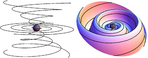
The Michel monopole, with central star drawn in. On the left, some representative lab frame magnetic field lines. On the right, the current sheet in the inclined case, with tangent field lines drawn in black. The pattern of the sheet rotates rigidly with the star, or equivalently moves radially outwards at the speed of light.
6.3.2 Inclined split monopole
We may equally well consider the inclined case, with the star magnetized in a split-monopole pattern with the split along an equator inclined at an angle α to the rotation axis |$\hat{\bf z}$| and corotating with the star. This provides a model for a pulsar with inclined magnetic axis.
The dipolar split monopole is the most relevant split configuration for emulating a dipole pulsar, but a variety of other configurations are possible. For example, one may split the solution on cones of fixed latitude, as is clear from the field lines shown in Fig. 2. Having two such cones, say at latitudes where |$\cos \theta = \pm 1/\sqrt{3}$|, provides a rough imitation of a quadrupole pulsar. In this aligned case, the conical sheets are stationary, but it would be straightforward to determine the more complicated shapes and dynamics in the inclined case. Most generally, one may use any seed curve on the sphere at one time to construct a sheet, since the monopolar (radial) component of the Michel monopole ensures that all such curves are transverse to field lines. In this sense, one may consider a sphere of arbitrary split-monopolar magnetization.
6.3.3 Black hole split monopole
One may also split the black hole version of the Michel monopole, as done by BZ in their original paper. The procedure is precisely analogous to the case of flat spacetime discussed above. The BZ model involves splitting in the equatorial plane, equation (51) with FMichel replaced with FBZ (equation 47). The sheet extends all the way to the event horizon. In nature, a magnetized accretion disc could source a field, and the current sheet becomes a crude model of such a disc. However, Lyutikov has raised the interesting possibility that the gravitational collapse of a pulsar could form a split-monopole black hole magnetosphere, where the current sheet originally present outside the light cylinder (e.g. Fig. 4) meets the horizon. If so, then the split BZ model would directly describe an astrophysical magnetosphere, if only for a brief time before magnetic reconnection destroys the sheet.
Although only the equatorial splitting has been explicitly considered in the black hole context, the more general splits discussed in the previous section are also possible. In particular, the inclined equatorial split also yields equation (54), with FMichel replaced with FBZ (47). As argued by Lyutikov in the aligned case, it is conceivable that this solution could model a black hole newly formed from the gravitational collapse of an inclined pulsar.
6.3.4 Whirling split monopole
In the whirling case (43), as in the simple rotating case, any curve tangent to the sphere is transverse to field lines, and so is a valid seed curve for a splitting. Thus while we do not construct explicit examples, our results do cover the magnetosphere, including current sheet dynamics, of an arbitrarily whirling, arbitrarily split-monopole-magnetized, conducting sphere. Astrophysically, the whirling split monopole could be helpful for modelling emission (or lack thereof) associated with pulsar glitches, including the case where in addition to the magnitude the direction of angular velocity is modified.
6.4 Reflection split
The preceding picture of current sheet behaviour applies to sheets produced by simple rescalings of the field strength across the sheet (equation 49). While this type of sheet commonly appears (for example in the outer region of many pulsar magnetosphere models), Maxwell's equations admit other types of field discontinuities supported by a current sheet |${\cal S}$|, provided only that the pullback to |${\cal S}$| of the jump in F vanishes. For this type of discontinuity, the magnetic field is not necessarily tangent to the sheet, and there is no simple story regarding the location and dynamics of the current sheets.
A common example of such a discontinuity occurs in reflection-symmetric magnetospheres, where F is reflected across the equatorial plane, entailing an equatorial current sheet. The field at |$\cal S$|, the world volume of the equatorial plane, can be decomposed as F = F∥ + F⊥, where F∥ is the projection of F into |${\cal S}$| and is invariant under reflection, and F⊥ flips sign under reflection. F∥ comprises the magnetic field normal to and the electric field tangent to the symmetry plane, and F⊥ comprises the tangent magnetic field and the normal electric field. The jump in F across |${\cal S}$| is thus [F] = 2F⊥, and the pullback of this vanishes, so the jump condition on F is satisfied. For the other jump condition, note that the dual *F⊥ is entirely ‘parallel’, so the jump in *F is [*F] = 2 * F⊥ = K, which determines the surface current.
The aligned split monopole discussed in Section 6.3.1 is a special case of this construction. In that example, F∥ vanishes, so the effect of the reflection is an overall sign change. Examples with a non-zero normal component of the magnetic field (and tangential component of the electric field) are the pulsar magnetospheres considered in Gruzinov (2011) and Contopoulos, Kalapotharakos & Kazanas (2014), the black hole magnetospheres of Uzdensky (2005), and the paraboloidal magnetospheres of Blandford (1976) and BZ.
7 STATIONARY, AXISYMMETRIC MAGNETOSPHERES
We turn now from specific analytical models to a general treatment of stationary, axisymmetric force-free magnetospheres, relevant both to spinning stars and to black holes. This section consists primarily of a systematic review and derivation of the standard mathematical and physical results, but using new computational techniques and the conceptual framework developed in Section 3. It can be seen as a spacetime counterpart to the 3+1 presentation of MacDonald & Thorne (1982), using an extension to curved spacetimes of the Euler-potential methods developed by Uchida (1997b). With our systematic use of differential forms, the efficiency and elegance of Uchida's approach is fully realized. In the following sections, we apply these results to pulsar and black hole magnetospheres.
Our treatment is spacetime geometrical in the sense that we do not decompose tensors into spatial components and temporal components with respect to a time foliation. However, we make heavy use of the existence of a coordinate system in which the metric components are block diagonal and do not depend on the two ‘symmetry coordinates’. This hybrid technique of using spacetime objects, specifically differential forms, in concert with special coordinates, is both remarkably efficient for computations and revealing about the structure of the theory. Another source of the efficiency and simplicity is the avoidance of unnecessary introduction of metric dependence into the calculations, and of confining what metric dependence there is to the action of the Hodge dual operator and metric determinants. This is achieved by using the exterior derivative rather than covariant derivatives, integrating p-forms on p-surfaces, and using the Hodge dual operator.
7.1 2+2 decomposition of spacetime
7.2 Degenerate, stationary, axisymmetric fields
Field sheets are surfaces of constant ϕ1 and ϕ2, hence are labelled by a value of ψ and a value of ϕ2. If the field is magnetically dominated, as we assume from now on unless otherwise stated, the field sheets are timelike. A magnetic field line, defined with respect to t, is the intersection of a field sheet with a surface of constant t. Besides the ‘true’ magnetic field lines, one can also define poloidal field lines, which are just the ψ contours in the poloidal space. The bending of a true field line in the azimuthal direction, i.e. the variation of its φ coordinate at fixed t, is determined by ψ2. As explained below, ψ determines the polar magnetic flux, and the function ΩF(ψ) determines the angular velocity of the field lines.
In the following subsections, we expand on the interpretation and properties of the quantities introduced here.
7.2.1 Magnetic flux function ψ
In deriving equation (67), we have chosen the orientation dφ on the loop |$\mathcal {C}$|, which by Stokes’ theorem fixes the orientation for the 2-surface |$\mathcal {S}$| with respect to which the flux is defined. We will call this the flux in the ‘upward’ direction. To understand the name, consider flat spacetime in cylindrical coordinates (t, z, ρ, φ), and let |$\mathcal {S}$| be a disc of constant z. Then the orientation dφ on the boundary corresponds to the orientation dρ ∧ dφ for the disc. Given the spacetime orientation dt ∧ dz ∧ dρ ∧ dφ, this corresponds to the flux of the magnetic field pseudo-vector using the surface-normal + ∂z.
The potential ψ is also related to the electrostatic potential as follows. A particle of mass m and charge e in stationary gravitational and electromagnetic fields has a conserved energy ξ · (mU + eA), where ξ is the stationary Killing vector, U is the particle four-velocity, and A is a vector potential that is invariant under the symmetry, |${\cal L}_\xi A = 0$|. Then it is natural to define ξ · A as the ‘electrostatic potential’. Although not gauge invariant, under a gauge transformation A → A′ = A + dλ this changes by ξ · dλ, which must be a constant if |${\cal L}_\xi A^{\prime }$| is to vanish. Hence, the electrostatic potential difference between two points is gauge invariant. For the degenerate fields discussed here, we may use A = ψ dϕ2, so that the electrostatic potential is − ΩF(ψ)ψ. This determines the ‘potential drop’ between magnetic field lines.
7.2.2 Polar current I
7.2.3 Angular velocity of field lines ΩF(ψ)
The stationary axisymmetry implies that the field F is unchanged by a shift in φ and/or t; however, the potential ϕ2 is in general unchanged only by a combined, helical shift (Δt, Δφ = ΩF(ψ)Δt). Under such a helical shift, the two Euler potentials are both unchanged, so a field sheet maps into itself. We may therefore interpret ΩF(ψ) as the angular velocity of the field line, the latter being defined by the intersection of the field sheet with a surface of constant t.
7.2.4 Corotation 1-form η
7.2.5 Light surfaces
At a point where η and χF are null, the corotating observer would need to travel at the speed of light. For this reason, a surface composed of such points is generally called a light surface, other names being critical surface, singular surface, velocity-of-light surface, or light cylinder.19 The latter name stems from the fact that in flat spacetime, with ΩF = const, there is one light surface located where the cylindrical radius is equal to 1/ΩF.
Light surfaces in magnetospheres play a significant role for two reasons. One is that the equation satisfied by the magnetic flux function (the so-called stream equation, cf. Section 7.4) has a critical point at a light surface. The implications of this for solutions of the equation are described briefly in Section 7.4.2.
The other role of light surfaces is that they determine causal boundaries of propagation of charged particle winds and Alfvén waves. As explained in Section 3.2.3, the field sheet metric governs such transport. Where the corotation vector χF is null, it coincides with one of the two field sheet light rays delineating the light cone on the sheet. Since χF is strictly toroidal, the light surface is evidently a causal boundary (at least locally) for either ingoing or outgoing motion on the sheet. In the case of the Michel monopole solution (41), for example, outside the light cylinder particles can propagate only to larger radii. For field sheet modes, the light cylinder is thus a horizon, beyond which influences cannot affect the interior.
In a general stationary, axisymmetric magnetosphere, the allowed direction of particle flow across the light surface, i.e. the direction of the other future pointing light ray on the field sheet, is the same as the direction of positive angular momentum flow in the field if ΩF is greater than ΩZ, the angular velocity of the local zero angular momentum observer (ZAMO). If instead ΩF < ΩZ, these directions are opposite. This is demonstrated in Section 7.3.1.
7.2.6 Field sheet Killing vector
As explained in Section 3.2.3, the field sheet metric governs the propagation of collisionless charged particles and Alfén waves in a certain approximation. The field sheet Killing vector thus provides conservation laws for these sorts of transport. In particular, there is a conserved quantity χ · p = pt + ΩFpφ associated with each particle or wavepacket trajectory, where p is the four-momentum or wave four-vector, respectively. Since the field sheet metric is two-dimensional, the single conserved quantity is enough to completely determine the motion from a choice of initial position and velocity. In applications, such initial conditions may be provided e.g. by particle injection velocities at non-degenerate gaps in an otherwise force-free magnetosphere. The four-velocity u of a particle at any point is then determined by the equations u2 = −1, u · F = 0, and |$u_a \chi _{\rm F}^a={\rm const}$|.
In flat spacetime, the conserved quantity for particles moving along field lines is |$u_a\chi _{\rm F}^a=\gamma (-1+ \Omega _{\rm F} \rho \, v_\varphi )$|, where γ is the Lorentz factor of the trajectory (in the rest frame defined by ∂t), ρ is the cylindrical radius, and vφ = ρ dφ/dt is the azimuthal three-velocity. This quantity is sometimes used to determine outflow velocities from force-free solutions (e.g. Contopoulos, Kazanas & Fendt 1999, equation 16). We have obtained the conserved quantity as a simple consequence of the existence of a Killing vector on the field sheets, a formulation that generalizes to arbitrary circular spacetimes.
We note that the intersection of a light surface with a given field sheet is a Killing horizon for the field sheet Killing vector. That is, it is a null curve to which the Killing vector is tangent. As mentioned in Section 5.1.1, in the case of the Michel monopole, the field sheets are isometric to two-dimensional de Sitter space, and the light cylinder horizon is a de Sitter horizon.
7.3 Energy and angular momentum currents
When the electromagnetic field is coupled to charges, the energy and angular momentum currents (74) and (75) are not conserved, unless the four-force vanishes along ∂φ and ∂t, respectively. Since the second terms in equations (74) and (75) are automatically conserved for stationary axisymmetric fields (see note below equation 72), conservation of energy and angular momentum amounts to the condition dψ ∧ d * F = 0. (In particular, if a stationary, axisymmetric, degenerate field conserves one of these, it also conserves the other.) This is equivalent to the first of the two force-free equations (26) or, equivalently, conservation of the first Euler current (27).22
7.3.1 Direction of particle flow at a light surface
We now establish the result mentioned in Section 7.2.5 that the direction of particle flow across a light surface is the same or opposite to the direction of positive angular momentum flow, according to whether ΩF − ΩZ is positive or negative. Here ΩZ is the ZAMO angular velocity discussed beginning with equation (87) below.
7.4 Stream equation
Up to now our discussion of stationary, axisymmetric fields has assumed degeneracy of the field, but has not assumed that it is force free. For force-free fields, the stream function ψ satisfies a non-linear partial differential equation which is known by many names: stream equation, Grad–Shafranov equation, transfield equation, and, in flat spacetime, pulsar equation (Michel 1973; Scharlemann & Wagoner 1973; Okamoto 1974; BZ). We will call this equation the stream equation, and we now derive it in the case of a general stationary, axisymmetric metric of the block diagonal form (55). A similar equation can be derived in the presence of other sorts of symmetries.
It is worth mentioning that the stream equation can apply more generally than in the stationary axisymmetric case. In particular, for any 2 + 2 metric, if the field is symmetric under one of the factors of the 2 + 2, and falls into Uchida's case 1 (Appendix D2), then the same manipulations above will give rise to a stream equation that differs only in minor details. For example, a stream equation applies to the case where the field is plane symmetric, i.e. x and y are the ignorable coordinates, while the fields depend on z and t, in flat spacetime.
7.4.1 Action derivation of stream equation
The stream equation can also be efficiently derived directly from the action (28), with the symmetric form (61) for the potentials. Uchida (1997a) worked this out and explained the relation to the Scharlemann–Wagoner action (Scharlemann & Wagoner 1973) from which the derivation is even simpler. Here we will briefly summarize Uchida's analysis using our methods.
7.4.2 Solution of the stream equation
The stream equation (86) for the stream function ψ has the peculiar feature that it contains unknown functions ΩF(ψ) and I(ψ) which must also be somehow determined. In this subsection, we briefly discuss the nature of this equation and mention several approaches to finding solutions.
These expectations are borne out in numerical calculations that iteratively update guesses for the free functions until a sufficiently smooth match is achieved across all light surfaces. This approach to solving the stream equation in the presence of light surfaces was introduced by Contopoulos et al. (1999) and later used by several other authors (Uzdensky 2005; Gruzinov 2006; Timokhin 2006; Contopoulos, Kazanas & Papadopoulos 2013; Nathanail & Contopoulos 2014). For a pulsar magnetosphere, ΩF(ψ) may be fixed in advance to be the (constant) angular velocity of the star (cf. Section 8.1), and the single free function I(ψ) may be determined by matching across the single light surface. Black hole magnetospheres are qualitatively different in three respects: (i) the location of the light surfaces generally depends on ΩF(ψ) and ψ, (ii) if the black hole is spinning, there can be two light surfaces (cf. Section 9.3), and (iii) at the horizon there is a fixed relation between ψ, I, and ΩF, the Znajek condition (cf. Section 9.1). The Znajek condition can be viewed as determining ψ on the horizon, given I(ψ) and ΩF(ψ). On field lines that cross both light surfaces, the latter two functions would also be determined.
In order to find analytic solutions to the stream equation, one approach is to restrict the dependence of ψ to a one-dimensional subspace of the two-dimensional poloidal space, converting the stream equation into an ordinary differential equation (ODE). Then, for example if ΩF is a fixed constant, the boundary condition on ψ can determine I(ψ) locally, leaving just an ODE to be solved. This kind of tactic was used for example by Menon & Dermer (2007), who found a family of solutions in the Kerr spacetime where ψ, ΩF, and I are independent of BL radial coordinate r.
Finally, stationary, axisymmetric force-free solutions can be generated by time-dependent evolution from non-force-free initial data, using numerical devices that short out electric fields and dissipate energy. Thus one effectively solves the stream equation through time-dependent evolution (e.g. Komissarov 2001; McKinney 2006; Spitkovsky 2006; Komissarov & McKinney 2007).
7.5 Field line topology
In this subsection, we establish two restrictions on the possible topology of magnetic field lines in stationary, axisymmetric force-free magnetospheres. In Sections 8 and 9, we apply the second of these results to pulsar and black holes magnetospheres.
7.5.1 No closed loops
We begin with the simpler of the two restrictions:
A stationary, axisymmetric, force-free, magnetically dominated field configuration cannot possess a closed loop of poloidal field line.
By a closed loop of poloidal field line we mean a level set of ψ that forms a smooth closed curve, i.e. a closed set ψ = const on which dψ ≠ 0. Note that such loops do not in general correspond to closed loops of ‘true’ field line, since those lines bend in the ∂φ-direction. To establish the result, we employ the expression (26) of the force-free condition in terms of the conservation of the Euler currents. In particular, we use the fact that the Euler current J2 = dϕ2 ∧ *F is a closed 3-form. By Stokes’ theorem, this implies the vanishing of the integral of J2 over any closed 3-surface bounding a force-free region of spacetime.
7.5.2 Light surface loop lemma
In this subsection, we prove a light surface loop lemma that will be useful when we treat pulsar and black hole magnetospheres. This lemma was part of the ‘no-ingrown-hair’ argument of MacDonald & Thorne (1982), but here we present it on its own and also discuss two related results. The lemma states that for stationary, axisymmetric, force-free fields (not necessarily magnetically dominated),
no poloidal field line may pierce a light surface twice in a contractible region where |$\Omega _{\rm F}^{\prime }=I^{\prime }=0$|
The condition |$\Omega _{\rm F}^{\prime }=0$| indicates that all field lines rotate with the same angular velocity, while I′ = 0 implies that no poloidal current flows in this region (otherwise I, being the total current through the cap with boundary at ψ, would depend on ψ). Our hypotheses allow non-zero toroidal magnetic field I, supported by poloidal current flowing elsewhere in the magnetosphere.
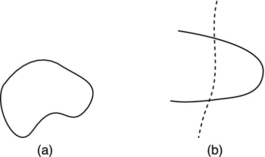
Disallowed topologies of force-free poloidal magnetic field lines. (a) No closed loops when magnetically dominated. (b) No light surface loops when |$\Omega _{\rm F}^{\prime }=I^{\prime }=0$|.
If more than one light surface is present, then, for any field line segment that pierces a single light surface twice (or more), there will also be a subsegment that pierces a (possibly different) light surface twice without encountering any other light surface. We may then run the above argument on that subsegment, again concluding that the field configuration is impossible. This establishes the lemma.
The conclusion of the light surface lemma also holds in two additional cases. First, since it is the product |$\Omega _{\rm F}^{\prime }\langle {{d}}t,\eta \rangle$| that appears in the stream equation (85) or (86), we may replace the assumption |$\Omega _{\rm F}^{\prime }=0$| with 〈dt, η〉 = 0. The interpretation of 〈dt, η〉 = 0 is that field lines corotate with ZAMOs, cf. equation (89).
Secondly, we may drop the force-free assumption and instead assume that (i) angular momentum is conserved (first force-free condition is satisfied and hence I = I(ψ)) and (ii) there is a reflection isometry28 (of the spacetime and the fields) about a spacelike 2-surface (poloidal curve flowed in toroidal directions) intersecting the light surface loop. The reflection isometry implies that I is odd under reflection (see equation 65, noting that F is even while ϵP is odd), but I = I(ψ) and the evenness of ψ implies that I is even. Thus we in fact have I = 0, and the assumption I′ = 0 is superfluous. We must still include |$\Omega _{\rm F}^{\prime }=0$| as an assumption, and in this case we still have the last equality in equation (99), dϕ2 ∧ d * F = d(|η|2* dψ). These quantities are now not known to vanish, but we may use the reflection isometry to argue that their integrals do vanish. To do so note that dϕ2 is even (first use the evenness of η and F to establish evenness of dψ, and then F = dψ ∧ dϕ2 implies dϕ2 is even), while d * F is odd on account of the duality. Thus the form dϕ2 ∧ d * F is odd. Since the shape of the light surface loop is symmetric, the integral of this form over the interior of the loop (flowed in φ and t to form a four-volume) is vanishing. This establishes the first line of equation (100), and the same arguments establish a contradiction. To summarize, we have shown that for stationary, axisymmetric, reflection-symmetric, degenerate energy- and angular-momentum-conserving fields with |$\Omega _{\rm F}^{\prime }=0$| (or 〈dt, η〉 = 0), no light surface loops straddling the reflection surface may exist.
7.6 Special case: no poloidal field
An example of this limit is provided by the Michel monopole solution − qd(cos θ)∧(dφ − ΩFdu). In the limit q → 0, ΩF → ∞, with qΩF held fixed. The vacuum monopole term (which provides the poloidal magnetic field) vanishes, leaving just the stationary, axisymmetric outgoing Poynting flux solution (30), F = qΩFd(cos θ)∧du, which satisfies the stream equation (103) rather than the generic stationary axisymmetric stream equation. Euler potentials for this solution in the above notation are specified by χ = qΩFcos θ and χ2 = −r.
Another interesting example arises in the Menon–Dermer solution, i.e. the stationary axisymmetric case of the Poynting flux solution (34) in Kerr spacetime (35), |$A(\theta )d\theta \wedge ({{d}}u - a\sin ^2\theta \, {{d}}\bar{\varphi })$|. That solution falls in the generic class on account of the |${{d}}\bar{\varphi }$| term, but since that term vanishes along the axis, the axis limit lands on this special case. The angular velocity of the field lines in this solution is ΩF = 1/(asin 2θ), whose limit indeed diverges as the axis is approached.
The case of no poloidal field does not appear to have been previously considered in the force-free context. However, Gourgoulhon et al. (2011) have given a completely general treatment of stationary, axisymmetric equilibria in the context of ideal MHD, which includes the magnetically dominated force-free case as a limit.
8 PULSAR MAGNETOSPHERE
This section addresses general features of magnetospheres around conducting, magnetized stars in the case of aligned rotation and magnetic axes. Such a configuration is stationary and axisymmetric, so does not pulse; however, it serves as a simple example of key properties of pulsar magnetospheres, and as an approximation for a nearly aligned pulsar. Specifically, we discuss the boundary condition at the stellar surface which determines the angular velocity ΩF(ψ) of the field, and the roles of the light cylinder and current sheet in delimiting the region of closed field lines.
The pulsar magnetosphere has mainly been studied in flat spacetime. We will discuss general features of pulsar magnetospheres based on the general metric (55), so our comments will hold when gravity is included. Our analysis also serves to identify precise circumstances under which each particular feature must hold.
8.1 Angular velocity of field lines
The angular velocity of field lines ΩF may be determined by the assumption of a perfectly conducting stellar surface, which should be a good approximation for neutron stars. If U is the four-velocity field of a perfectly conducting surface, then the contraction of U · F with any vector tangent to the surface vanishes. That is, the electric field in the rest frame of the conductor must have no component tangent to the surface. If the surface is that of an axisymmetric star with four-velocity U∝∂t + Ω∂φ, then for a stationary, axisymmetric degenerate field (62) we have U · F = −(U · η)dψ∝(ΩF − Ω)dψ. Provided the poloidal magnetic field is not tangent to the stellar surface (i.e. provided there is a surface tangent vector v with v · dψ ≠ 0), it follows that Ω = ΩF. We have thus shown that for stationary, axisymmetric, degenerate fields,
poloidal field lines that non-tangentially intersect a perfectly conducting star must have ΩF = Ω
Thus the field lines corotate with the star. Note that when Ω = ΩF we have U · F = 0 (see expression in text above), implying that also the normal component of the electric field in the rotating frame must vanish at the surface of the conducting star. Thus there is no induced charge on the stellar surface, according to corotating observers. Static observers, on the other hand, will generically measure induced charge, depending on the assumptions for the field configuration within the star.
The lack of induced surface charge in the rotating frame is a direct consequence of degeneracy and the conducting boundary condition: since the tangential components must vanish on the conducting surface, the electric field is purely normal. But if the magnetic field has a normal component, |$\boldsymbol E\cdot \boldsymbol B=0$| implies that the electric field vanishes entirely, and there is no induced charge. If the star were instead surrounded by vacuum, the field would not be degenerate, and generically there would be a surface charge and a normal component of the electric field in the rotating frame.
8.2 Open and closed zones
Closed field lines are defined to be field lines that intersect the star twice, while open field lines intersect it once. In vacuum, the field lines of a monopole star would all be open, while those of a dipole are all closed. The standard aligned force-free pulsar magnetosphere (Fig. 4), on the other hand, is a mix: the field lines form a dipole pattern at the star, but only some of them return to close, with the rest opening up to infinity. This basic structure of closed and open zones was postulated in the earliest work on the subject (Goldreich & Julian 1969), and later work has confirmed that such solutions do exist.
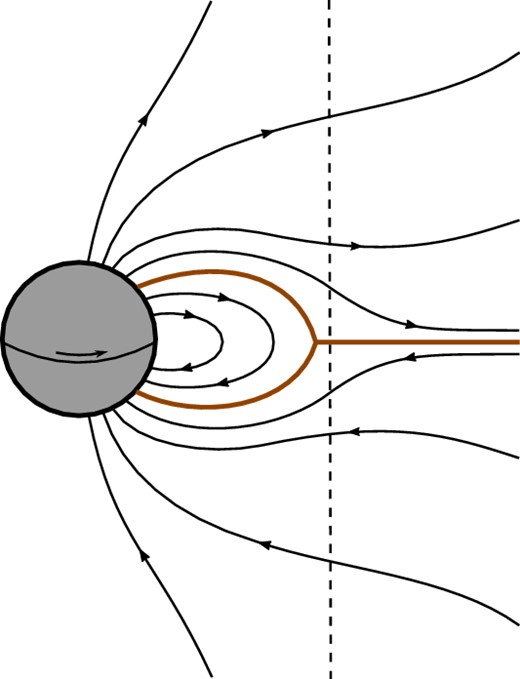
Diagram illustrating the poloidal structure of the standard aligned pulsar magnetosphere. A current sheet (thick brown line) separates poloidal field lines (black) into three zones, one closed and two open. The closed zone terminates at, or just within, the light cylinder (dashed line, shown artificially close to the star).
An important feature of all configurations previously considered is that the closed field lines remain within the light cylinder,29 unless they pass through a non-force free region such as a current sheet. While it is commonly asserted that closed force-free field lines must remain within the light cylinder, we are unaware of any explicit demonstration in the literature. In this section, we will critique the reasoning that one often hears or reads, and then demonstrate several related results based on various specific assumptions. We will conclude by explaining why, despite these results, the possibility that closed force-free field lines could venture outside the light cylinder has not (yet) been ruled out.
An argument one often hears or reads for the impossibility of closed magnetic field lines in a degenerate field outside the light cylinder is based on the notion that particles stuck on such field lines (in cyclotron motion) would have to be moving faster than the speed of light. It seems unsatisfactory to invoke ‘particles’ to determine something about force-free fields, however, since the matter plays no role in the dynamics of those fields (other than to carry the current). To the extent that such an argument is valid, it should be possible to reformulate it without reference to particles.
To identify such a reformulation, we note that (i) particles are stuck on field lines only if the field is magnetically dominated, and (ii) such field lines always admit subluminal particles stuck on them, because magnetically dominated, degenerate fields always have timelike field sheets. Hence, to rule out some behaviour of a degenerate field ‘because particles stuck on field lines cannot go faster than light must be logically equivalent to ruling it out simply by the assumption that the field is magnetically dominated. In what follows, we will base our arguments on magnetic domination rather than considerations of particles. We will also give one argument that does not require magnetic domination.
A stationary, axisymmetric field cannot remain magnetically dominated outside the light cylinder if the field line has no toroidal component, because such a line sweeps out a spacelike field sheet outside the light cylinder. To reach this conclusion computationally, note that the absence of a toroidal magnetic field is equivalent to the condition I = 0 (cf. equation 65), which implies F2 = |dψ|2|η|2 (equation 66). The factor |dψ|2 is non-negative, since the poloidal subspace is Riemannian, and outside the light cylinder |η|2 < 0 by definition, so if I = 0, then F2 must be negative (or zero) outside the light cylinder, violating magnetic domination. This establishes a link between the absence of polar current and the confinement of magnetic field lines:
In a stationary, axisymmetric, degenerate, magnetically dominated field configuration, field lines with I = 0 must lie within the light cylinder.
The idea that closed field lines must remain within the light cylinder may in part be due to an association between closed field lines and I = 0. The original Goldreich–Julian model postulated a corotating portion of the magnetosphere, where one sign of charge rotates rigidly with the star. This portion indeed has I = 0, since there is no poloidal current. In most self-consistent models constructed by solving the stream equation (e.g. Contopoulos et al. 1999), I = 0 is assumed in the closed zone. One possible reason for this assumption is the fact that
reflection symmetry and the force-free condition imply that closed field lines crossing the equatorial plane must have I = 0.
By ‘reflection symmetry’ we mean an isometry of the spacetime and fields under which the volume element ϵ changes sign, and which leaves fixed a 3-surface composed of a spacelike 2-surface flowed along the timelike Killing field. In flat spacetime, this corresponds to the usual reflection symmetry about the plane z = 0, and in the general case, we refer to the spacelike 2-surface as the equatorial ‘plane’ although it would generally have intrinsic curvature. To establish the result, we note that I(ψ) is constant on the field line, hence is even under reflection, but it is also required to be odd since F (equation 65) is even while the poloidal area element ϵP is odd. Since this result relies only on I = I(ψ), it suffices to assume just that energy and angular momentum are conserved, rather than the full force-free condition (see discussion in Section 7.3 above).
Combining the previous two quoted statements, we have the following theorem on closed field lines:
In a stationary, axisymmetric, reflection-symmetric, force-free, magnetically dominated field configuration, field lines crossing the equatorial plane must have I = 0 and remain within the light cylinder.
Note that reflection symmetry implies that field lines which come from the star and cross the equator are closed, so this result provides a precise set of assumptions under which the basic topology of the standard pulsar magnetosphere is to be expected. Again, the force-free assumption may be replaced by that of conservation of energy and angular momentum. The assumption of magnetic domination can be replaced by the condition that |$\Omega _{\rm F}^{\prime }=0$| which, as shown in Section 8.1, necessarily holds if the field terminates on a rigidly rotating, perfectly conducting star with non-tangential poloidal surface field. Then, together with the other assumptions, the light surface loop lemma of Section 7.5.2 applies and establishes that closed lines cannot extend outside the light cylinder. We thus have the following alternate result:
In a stationary, axisymmetric, reflection-symmetric, force-free, field configuration with |$\Omega _{\rm F}^{\prime }=0$|, field lines crossing the equatorial plane must have I = 0 and remain within the light cylinder.
Given the above considerations about closed field lines, a natural (and so-far standard) configuration for the dipole pulsar magnetosphere is that shown in Fig. 4. Field lines near the equator of the star would, in vacuum, have returned more quickly to the star, so it stands to reason that the closed zone of the configuration will be near the equator. On the other hand, field lines near the poles would have extended far from the star in vacuum, so it makes sense that in the force-free case these field lines will open up to infinity. Outside the light cylinder, there are no closed field lines, and the reversal of the sign of the field across the equator implies the presence of a current sheet (see Section 6). A current sheet is also present at the boundary between closed and open zones, connecting to the star. This general structure of the aligned dipole pulsar force-free magnetosphere has become standard, but alternative models do exist (Gruzinov 2011; Contopoulos et al. 2014).
We conclude this section with a discussion of situations in which closed field lines could be present outside the light cylinder in a magnetically dominated field configuration. We first discuss fields that are assumed to be degenerate but are otherwise arbitrary. In this case, it is straightforward to construct closed zones that proceed outside the light cylinder, since ψ, ΩF(ψ), and I may be chosen freely. In particular, we may take ΩF = const, choose ψ corresponding to the standard closed/open structure of the pulsar magnetosphere except with the closed zone penetrating the light cylinder, and then choose I large enough that F2 is positive everywhere in the closed zone (see equation 66). This configuration must violate reflection symmetry, but by a similar construction we may form closed loops outside the light cylinder in a reflection-symmetric magnetosphere by confining those loops to a hemisphere.
A more interesting example is provided by the new pulsar magnetosphere of Contopoulos et al. (2014). There the field is magnetically dominated, reflection symmetric, satisfies |$\Omega _{\rm F}^{\prime }=0$|, and is force free everywhere except in the equatorial plane where lies a current sheet. There are closed field lines with I(ψ) ≠ 0 that extend outside the light cylinder and have a kink at the current sheet. This configuration escapes our no-go theorem because of the infinitesimally thin current sheet violating the force-free condition. Specifically, a non-zero current is consistent with reflection symmetry because I(ψ) flips sign across the current sheet. That is, Ibelow(ψ) = −Iabove(ψ). This reversal of the sign of I on a field line would not be allowed if the field were force free everywhere.
Adopting the additional constraint that the fields be everywhere force free has the potential to eliminate the possibility of closed poloidal field lines venturing outside the light cylinder, but we have not found an argument that does so. Gruzinov (2006) has found force-free solutions with closed lines having I ≠ 0, showing that there is no difficulty of the lines closing. He has chosen to study configurations where the closed lines remain within the light cylinder, but we see nothing preventing alternative configurations for which they do not. As far as we are aware, it is currently an open question whether magnetically dominated force-free fields can have closed field lines outside the light cylinder.
9 BLACK HOLE MAGNETOSPHERE
Force-free magnetospheres of spinning black holes differ qualitatively from those of stars because of the presence of the event horizon and ergosphere. Within a star, the force-free condition does not hold, so energy (and angular momentum) can be transferred from the star to the electromagnetic field. In the case of a stationary black hole, by contrast, the force-free condition may in principle hold up to and across the horizon, and conditions behind the horizon cannot affect the exterior, so there is no analogue of the star transferring energy to the field. On the other hand, the meaning of this conserved energy is modified because of the spacetime curvature: as discussed in Section 7.3, it is the integral of the Noether current associated with the ‘time-translation’ Killing vector. On a stationary spinning black hole spacetime, this Killing vector is timelike far from the black hole, but spacelike near the black hole in the ergosphere, due to the extreme ‘dragging of inertial frames’. In the ergosphere, therefore, Killing energy is actually spatial momentum as defined by local observers. Hence, the electromagnetic field can have a local negative Killing energy density. Killing energy can therefore be extracted from the black hole, despite its conservation, because a corresponding negative Killing energy can flow across the horizon into the black hole. A process in which rotational energy is extracted from a spinning black hole, with a negative Killing energy flux across the horizon balancing a positive Killing energy flux at infinity, is (or should be30) called a Penrose process (Penrose 1969, 2002). When the mechanism involves a force-free magnetosphere, it is generally known as the BZ process or mechanism. For further discussion of the relationship between the Penrose and BZ processes, see e.g. Komissarov (2009) and Lasota et al. (2014).
Another qualitative difference between stellar and black hole magnetospheres lies in the topology of their field lines. The main qualitative feature of the pulsar magnetosphere relative to vacuum is that some field lines are open, although some loop back on to the star. In the case of a spinning black hole, it turns out that all field lines extending from the horizon must be open, unless they enter or loop around a non-force-free region, such as an accretion disc. In reference to the ‘no-hair’ theorems on black hole uniqueness in vacuum, we name this result the no-ingrown-hair theorem. This illustrates the fact that while the magnetic field lines (hairs) may indeed emerge from the horizon of a black hole with a force-free magnetosphere, they may not return unless they encounter a non-force-free region. The no-ingrown-hair result was first derived by MacDonald & Thorne (1982); our proof is similar but uses some different arguments.
Finally, there is a tricky technical point that arises only in the treatment of black hole magnetospheres. The 2 + 2 poloidal/toroidal decomposition of the spacetime, which is so useful in handling the stationary axisymmetric force-free equations, breaks down at the horizon. One issue is that the 1-form dr becomes null (it is normal to the horizon, which lies at constant r), so that the poloidal subspace becomes null, rather than spacelike. Another is that the 1-forms dt and dφ diverge, both in a manner proportional to dr, so that the toroidal subspace also becomes null, with the same null direction as the poloidal subspace. One way to handle this is to instead use coordinates that are regular at the horizon. Alternatively, one can continue to use the 2 + 2 decomposition, being careful to determine the appropriate conditions that must be imposed to ensure regularity at the horizon. Here we will do some of both.
In this section, we adopt the Kerr metric for the black hole; however, the main important property is the presence of a horizon-generating Killing vector ∂t + ΩH∂φ, so analogous results could be easily derived for other spinning black hole metrics of the form (55).
9.1 Znajek horizon condition
To see that equation (104) is a relationship between invariants, recall that ΩF may be defined by the condition (∂t + ΩF∂φ) · F = 0 for degenerate fields F with ∂φ · F ≠ 0, the polar current I is the upward flow of charge per unit Killing time through a polar cap bounded by an axial loop, 2πψ is the upward flux of F through such a loop, and |$2\pi \sqrt{g_{\varphi \varphi }}$| is its circumference. These notions are valid on the horizon, where the remaining ingredient |$\psi _{,\theta }/\sqrt{g_{\theta \theta }}$| is the derivative with respect to proper length along the horizon in the direction orthogonal to the two Killing vectors, away from the upward pole.
When thinking of the intrinsic quantities I, ΩF, and ψ individually, we are unaware of any reason to expect them to be related on the horizon. However, since the poloidal and toroidal subspaces become null, and with non-trivial intersection in the limit at the horizon, the corresponding parts of the 2-form F are not independent. This makes the existence of the Znajek condition less surprising.
If the minus sign is chosen, then the fields are regular on the past horizon instead of the future horizon and thus represent a white hole magnetosphere rather than a black hole magnetosphere. Note that it is impossible for the fields to be regular on both horizons, since all quantities appearing in equation (125) take the same value on both horizons. The fact that equation (125) is always satisfied by smooth solutions to the stream equation indicates that, when solving the stream equation on r ≥ r+, the only boundary condition at r = r+ that one needs to impose is the sign choice corresponding to a black hole.
The Znajek condition has a number of practical applications. First, it can be used as a horizon boundary condition for the stream equation, as in the original BZ paper. (The BZ solution can equally well be derived without the use of the condition; cf. McKinney & Gammie 2004 and our Section 5.3.) The condition is also helpful in derivations of theoretical results. We use it to obtain the illustrative flux formulae (126) and (127) (following BZ) and to prove the no-ingrown-hair theorem (following MacDonald & Thorne 1982).
9.2 Energy and angular momentum flux
It also follows from equations (126) and (127) that any outflow of energy is accompanied by an outflow of angular momentum. This is consistent with the fact that the source of the energy is the rotation of the black hole. A universal upper limit to the energy extracted for a given angular momentum extracted can be found using the null energy condition, Tabℓaℓb > 0 for null vectors ℓa, which in particular is satisfied by the electromagnetic field stress tensor. Since the horizon-generating Killing field χ is null on the horizon, we have Tabχaχb ≥ 0 there. This expression is equal to the inward flux of energy |$T_{ab}\mathrm{\partial} _t^a \chi ^b$| minus ΩH times the inward flux of angular momentum |$-T_{ab}\mathrm{\partial} _\varphi ^a \chi ^b$|. It follows that the outward flux of energy is bounded by |$\delta \mathcal {E} \le \Omega _{\rm H} \delta \mathcal {J}$|. The BZ process satisfies |$\delta \mathcal {E} = \Omega _{\rm F} \delta \mathcal {J}$|, so its efficiency is governed by the ratio ΩF/ΩH.
As noted in the original paper, the process can be characterized in thermodynamic terms. The BZ process is stationary, but when the back reaction on the geometry is taken into account it becomes a quasi-stationary process in which the first law of black hole mechanics (Bardeen, Carter & Hawking 1973; Bekenstein 1973) should apply, δM − ΩHδJ = (κ/8π)δA, where M and J are the mass and angular momentum of the black hole, κ is the surface gravity, and A is the horizon area. The second law of black hole mechanics (which follows from the null energy condition and cosmic censorship) states that the area cannot decrease, δA ≥ 0 (Hawking 1972; Hawking & Ellis 1973; Penrose & Floyd 1971). In the BZ process, |$\delta M=-\delta \mathcal {E}$| and |$\delta J=-\delta \mathcal {J}$|, so the first and second laws imply the same upper bound obtained above using the null energy condition directly. Perfect efficiency corresponds to the case in which the area of the horizon is unchanged. According to the second law of black hole mechanics, only in that limit is the process reversible.
9.3 Light surfaces in a black hole magnetosphere
Recall that a light surface is a hypersurface in spacetime where the field sheet Killing vector χF = ∂t + ΩF(ψ)∂φ is null or, equivalently, where the corotation 1-form η is null. Light surfaces play a practical role in finding force-free solutions, since they correspond to singular points of the stream equation (see Section 7.4.2). They also act as horizons for the propagation of particles and Alfvén waves through the magnetosphere (see Section 7.2.5). In the Kerr spacetime, there are in general two light surfaces, an outer one qualitatively similar to the ordinary light cylinder, and an inner one within the ergosphere. Outside the outer light surface, a corotating curve with angular velocity ΩF is rotating too fast to be timelike, whereas inside the inner light surface, it is rotating too slowly to be timelike. The existence of the inner surface follows from the fact that within the ergosphere observers (i.e. timelike curves) must rotate with a minimum angular velocity, which approaches ΩH at the event horizon. Any field line with ΩF < ΩH will therefore cross an inner light surface at some point sufficiently close to the horizon. The inner light surface meets the horizon at the poles.
The field sheet Killing vector is spacelike inside the inner light surface and outside the outer one, and timelike in between. For ΩF < ΩH, wind particles and Alfvén waves can travel only inwards across the inner light surface and only outwards across the outer light surface, as indicated in Fig. 5. This follows from the analysis of Section (7.3.1), which established that the particle wind direction relative to that of positive angular momentum flow (126) is determined by the sign of ΩF − ΩZ, which is positive at the outer light surface and negative at the inner one. This was shown using a different method by Komissarov (2004), who has given a detailed discussion of the properties of the light surfaces of Kerr.
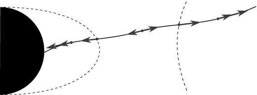
Diagram of black hole light surfaces (dashed lines) and wind propagation along a field line. The inner light surface is drawn exaggeratedly far from the black hole. Arrows indicate the projection of the field sheet null vectors on to the poloidal plane. These bound the possible poloidal velocities of particles moving on the field line. Particles may only move inwards inside of the inner surface, and only outwards outside of the outer surface.
9.4 No ingrown hair
We now prove the no-ingrown-hair theorem, which forbids regions of closed field lines for black hole magnetospheres (MacDonald & Thorne 1982). By a closed field line we mean a smooth poloidal field line that non-tangentially32 intersects the horizon twice, i.e. a level set of ψ on which dψ ≠ 0, which intersects r = r+ twice, each time with ψ, θ ≠ 0. We first establish that I = 0 and ΩF = ΩH for a closed field line in a force-free region. (We use only the first force-free condition I = I(ψ) for this part of the argument.) The regularity condition (104) implies that the sign of I is determined by the product of ΩF(ψ) − ΩH, which is the same at the two ends (and everywhere on the line), with ψ, θ, which has opposite sign at the two ends (since loops with different values of ψ are nested and θ is monotonic along the horizon). Thus I has opposite sign at opposite ends; however, I is also constant on the line, and hence must vanish. The regularity condition (together with ψ, θ ≠ 0) then implies that ΩF = ΩH for the line.
In a force-free region of closed field lines, we thus have |$\Omega _{\rm F}^{\prime }=I^{\prime }=0$|, so the conditions for the light surface loop lemma hold. Furthermore, since ΩF = ΩH, the horizon itself is a light surface [recall that the Killing vector (105) is null at the horizon], and the lemma applies to it. This proves the no-ingrown-hair theorem:
A contractible force-free region of closed poloidal field lines cannot exist in a stationary, axisymmetric, force-free Kerr black hole magnetosphere.
Thus a black hole cannot have a ‘closed zone’ like a dipole pulsar does. Note that the theorem does not rely on reflection symmetry or magnetic domination.
Closed field lines may exist if they pass through, or loop around, non-force-free regions of the magnetosphere. For example, closed field lines may connect the black hole to an accretion disc. Or if a torus of material orbits the black hole, field lines may loop around the torus before returning to the horizon. (These looping field lines must still have ΩF = ΩH and I = 0.) The no-ingrown-hair theorem is a natural generalization to the force-free setting of the no-hair idea that an astrophysical black hole cannot have its ‘own’ magnetic field. In order for closed field lines to exist, non-force-free currents must flow to support them. These ideas are illustrated in Fig. 6.
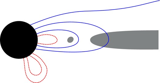
Allowed (blue solid) and disallowed (red dashed) topologies of poloidal field lines in a force-free black hole magnetosphere. Open lines are allowed. Closed lines must pass through, or loop around, a non-force-free region (grey).
Like its classical counterpart, the no-ingrown-hair theorem deals only with stationary situations, giving no insight into how any closed loop will be destroyed during the approach to stationarity. It seems likely that loops will either be absorbed by the black hole (Thorne, Price & MacDonald 1986) or opened up by non-force-free processes (Lyutikov & McKinney 2011). Qualitative discussions of different field line types in black hole magnetospheres can be found in Thorne et al. (1986), Blandford (2002), Hirose et al. (2004), and McKinney (2005).
We are grateful to Julian Krolik, Luis Lehner, Jon McKinney, and Cole Miller for many helpful conversations. TJ is grateful for hospitality at the Institut d’Astrophysique de Paris, where some of this research was conducted. This research was supported in part by Perimeter Institute for Theoretical Physics. Research at Perimeter Institute is supported by the Government of Canada through Industry Canada and by the Province of Ontario through the Ministry of Research & Innovation. SG acknowledges support from NASA through the Einstein Fellowship Program, grant PF1-120082. TJ was supported in part by the NSF under grant no. PHY-0903572.
While the bulk of the magnetosphere should be force free, small violating regions of two types can exist. First, regions where particles are produced may expel those particles with high velocity, so that plasma density high enough to achieve |$\boldsymbol {E} \cdot \boldsymbol {B}=0$| is never attained in those regions. Such regions are called gaps, and may provide a source of the high-energy particles observed in the pulsar wind. Secondly, as we discuss in some detail later, force-free fields tend to produce thin sheets of current where the field is not force free.
Curiously, for any degenerate field, the magnetic field defined by arbitrary observer, |$B^d = {\textstyle {\frac{1}{2}}}\epsilon ^{abcd} F_{ab} U_c$|, lies in the kernel of F, since F[abFd]e = F[abFde] = 0.
The submanifolds were called ‘flux surfaces’ by Carter and Uchida. We prefer the name field sheet because of the connotation of time evolution suggested by the similarity with the term ‘worldsheet’, which is appropriate in the magnetic case. We note also that the term ‘flux surface’ is commonly used in another sense, to describe a spacelike 2-surface to which the magnetic field is everywhere tangent.
These Euler currents are the Noether currents associated with the global symmetries ϕ1 → ϕ1 + f1(ϕ2) and ϕ2 → ϕ2 + f2(ϕ1) of the action (28).
An alternate approach (Thompson & Blaes 1998; Buniy & Kephart 2014) is to supplement the usual Maxwell action for the vector potential with a Lagrange multiplier term enforcing the degeneracy condition, |$S= -\frac{1}{2}\int F\wedge \ast F -\lambda F\wedge F$|. The resulting Euler–Lagrange equations are d * F = dλ ∧ F and F ∧ F = 0, another formulation of FFE. We learn from this that J = dλ ∧ F = dλ ∧ dϕ1 ∧ dϕ2 for some scalar field λ, which immediately implies the force-free condition (26). (Conversely, it is possible to show that J has this directly from the force-free conditions 24 and dF = 0.)
Monopole charge is conventionally defined to equal the flux integral. Our q is thus 1/4π times the usual notion; we nevertheless refer to q as the monopole charge.
The discontinuity could be avoided by using instead the potential Amon = −qcos θ dφ. However, the norm of the 1-form dφ is (gφφ)1/2 = 1/(rsin θ), which blows up at the poles. This can be fixed at the north pole by using instead Amon, N = −q(cos θ − 1) dφ and at the south pole by using Amon, S = −q(cos θ + 1) dφ, which differs from the northern potential by the pure gauge piece −2q dφ. The discontinuity of φ implies that this gauge transformation is not trivial however, which accounts for the existence of a non-zero magnetic flux through the sphere.
The concept of Killing time applies to an individual integral curve of the Killing field ξa, and is given by the lapse of λ along the curve, where λ is any function satisfying ξa∇aλ = 1 on the curve. In Schwarzschild, possible choices for λ include the usual time coordinate t as well as the outgoing and ingoing Eddington–Finklestein coordinates u and v. The Killing time may equivalently be defined as the lapse of parameter along the curve, when parametrized so that the tangent vector equals the Killing vector.
Note also that the solution is not regular on the future horizon unless dζ vanishes as u → ∞.
The reason for this can be traced to force-free condition |$\boldsymbol E\cdot \boldsymbol j =0$| (equation 6). Since the current is radial, this condition implies that |$\boldsymbol E$| has no radial component, which implies that the flux of |$\boldsymbol E$| through a sphere vanishes, so there can be no net charge inside the sphere.
In Kerr, the time-reverse refers to sending t → −t and φ → −φ.
The exact magnetic monopole solution on Kerr is obtained by taking the dual of the solution generated by the vector potential Aa = ξa, where ξa is the (asymptotic) time-translation Killing field.
The vector ∂r is defined in the (u, r, θ, φ) coordinate system, so it corresponds to translation of r at fixed u, θ, φ, and hence is a future pointing, outgoing null vector.
When perturbing a vacuum solution F(0) to a force-free solution F(0) + F(1), the first-order force-free condition is simply F(0) · j(1) = 0. Thus one may choose any conserved current j(1) transverse to the background field and then construct an associated Maxwell field d * F(1) = *j(1). BZ eliminated this freedom by demanding that perturbative solutions approach a genuine non-linear force-free solution (in this case the Michel monopole) at large r. Here we simply promote the Michel solution to Kerr and note that the field equations hold to O(a).
Such sheets are supported in simulations by (non-force-free) prescriptions that enforce magnetic domination.
There is no loss of generality in assuming that the symmetries commute (Carter 1970), and for asymptotically flat solutions to Einstein's equation in vacuum or with a circularly rotating fluid source, the 2-surface orthogonality property necessarily holds (Wald 1984). Non-circular spacetimes result from gravitational effects of meridional matter flow or toroidal magnetic fields (Gourgoulhon & Bonazzola 1993). A fully geometrical treatment of ideal MHD in stationary, axisymmetric spacetimes, allowing for non-circularity, is given in Gourgoulhon et al. (2011).
In cylindrical coordinates in flat spacetime for a disc of constant z, this corresponds to the orientation dt ∧ dφ ∧ dρ on |$\mathcal {S} \times \Delta t$|, which, given the spacetime orientation dt ∧ dφ ∧ dρ ∧ dz, corresponds to flux along the + ∂z-direction.
We caution the reader that some authors reserve the term ‘light surface’ for a place where F2 vanishes. These two notions of light surface agree only when I = 0 (see equation 66).
The existence of this symmetry of the Euler potentials is an example of a general property, discussed in Appendix D, which holds for degenerate fields with two commuting symmetry vectors X and Y, provided the (constant) quantity X · Y · F is non-vanishing.
The total four-momentum vector Pa is defined by |$\int {\cal J}_\xi = - \eta _{ab} P^a \xi _\infty ^b$|, so that the time and space components of Pa, which define the energy and translational momentum, have opposite signs in relation to the corresponding ‘Hamiltonian’ |$\int {\cal J}_\xi$|.
This property also holds for configurations with a single symmetry: for a degenerate EM field that is Lie derived by a Killing field ξ of the background spacetime, conservation of the current conjugate to ξ is equivalent to the force-free condition involving the potential that is invariant under the symmetry. This follows from equation (106) and the analysis of Appendix D1.
In the electrically dominated case, we instead have that poloidal current flows along poloidal equipotentials, i.e. perpendicular to electric field lines.
uZ is future pointing timelike at infinity, is timelike everywhere (since it is orthogonal to the spacelike vector ∂φ and lies in the toroidal plane), and is nowhere zero. Hence, it is future timelike everywhere.
For Dirichlet data, choosing I(ψ) and ΩF(ψ) is equivalent to specifying I and ΩF on the boundary. Thus the total boundary data are a component of the poloidal magnetic field (derived from ψ), a component of the poloidal electric field (obtained from ΩF and ψ), and the toroidal magnetic field (proportional to I).
If |η|2 vanishes quadratically or faster, the equation would actually be zeroth order, i.e. algebraic. However, this situation does not arise in practice.
A definition of a reflection isometry is given in Section 8.2.
To model pulsars, we focus on spacetimes for which degenerate field configurations will have a single light surface with the topology of a cylinder, outside of which corotating trajectories are spacelike. We refer to this surface as the light cylinder.
The term is sometimes reserved for a particular class of such processes. However, while Penrose introduced the idea with the example of lowering a mass into the ergosphere at the end of a rope, he concluded that ‘Thus, in a sense, we have found a way of extracting rotational energy from the “black hole”. Of course, this is hardly a practical method! Certain improvements may be possible, e.g. using a ballistic method.7 But the real significance is to find out what can and what cannot be done in principle since this may have some indirect relevance to astrophysical situations.’. (His footnote 7 states ‘Calculations show that this can indeed be done’, and goes on to describe the particle splitting method, now usually called the Penrose process).
To determine the sign of ⋆χ, note that on the future horizon χa ∼ (du)a (both 1-forms are null and normal to the horizon). As shown at the end of Appendix A2.3, in the Schwarzschild case, ⋆du = du; hence, ⋆χ = χ. The Kerr case is related by a continuous deformation to Schwarzschild, so the sign is the same. On the past horizon, χa ∼ (dv)a and ⋆dv = −dv; hence, ⋆χ = −χ.
In earlier discussion, we did not include this additional proviso as part of the definition of ‘closed field line’. Note, however, that non-tangential intersection is necessary for establishing that conductors determine the rotation frequency of their field lines (see Section 8.1).
Given a spacetime orientation ϵ, a direction of flow across a three-surface Σ corresponds to an orientation v · ϵ on Σ, where v is any vector transverse to Σ sharing the flow direction. The integral |$\int _\Sigma J$| with respect to this orientation gives the current flowing across Σ in the sense of v.
The surface orientation ϵ2 is related to a vector a defining the ‘outward’ direction for the flux by ϵ2 = a · (u · ϵ) (up to positive rescalings), where u is a future timelike vector and ϵ is the spacetime orientation.
An eternal black hole provides an example with non-trivial homology. If the black hole carries a magnetic monopole charge, then the fluxes through two surfaces spanning a loop will not be the same if the two surfaces together enclose the horizon.
REFERENCES
APPENDIX A: DIFFERENTIAL FORMS
A1 Integration of forms
A2 Hodge dual operator
To begin with an intuitive definition, the Hodge dual * of a decomposable p-form is simply the orthogonal decomposable form with the same squared norm, up to a sign. The sign of the squared norm of the dual is opposite in four dimensional spacetime, because the dual of a spacelike form is timelike, and vice versa. This definition is extended linearly to linear combinations of such forms, and it defines the dual of a form up to a sign. A more precise definition fixes all of these signs, up to one overall sign that depends on the choice of an orientation. Keeping track of the signs can be tedious, but for many purposes they need not be determined. The dual of the dual *2 brings one back to the same form, up to a sign that depends on the dimension of the space, the rank of the form, and the signature of the metric. In two- or four-dimensional Lorentzian spacetime, *2 = ±1, with the + sign for odd rank forms and the − sign for even rank forms, while for Euclidean signature the signs are opposite to these.
A2.1 Diagonal metrics
A2.2 Orthogonal subspaces
A2.3 Dual of a null 2-form
A2.4 Dual of a null 3-form
A3 Electromagnetism and differential forms
The integral of the 2-form F on a spacelike 2-surface is the magnetic flux through that surface. The choice of orientation for the surface integral corresponds in 3+1 terms to the choice of sign for the normal to the surface when defining the flux of the magnetic field pseudo-vector.34 This integral vanishes if the 2-surface is the (closed) boundary of a three-ball and dF = 0 holds everywhere in the interior. The magnetic flux through two homologous surfaces bounded by the same loop must therefore be the same, so the flux through a loop is well defined.35
The jump conditions (A23) are established by integrating Maxwell's equations (A21) and (A22) over the thickened patch and using Stokes’ theorem, in the limit that the width of the thickening goes to zero. It is easily checked that for a surface at rest in an inertial frame in flat spacetime, these conditions agree with the familiar ones: the tangential electric field and normal magnetic field must be continuous, the jump in the normal electric field is the surface charge density, and the jump in the tangential magnetic field is the cross product of the surface current density with the unit normal to the surface in the direction the jump is defined.
APPENDIX B: POYNTING FLUX EXAMPLES
The fact that stationary field configurations can carry energy away from a source in FFE is counter to intuition from the vacuum case, where this role is normally reserved for time-dependent fields sourced by accelerated charges. In order to have finite, non-vanishing net flux from a central source, the Poynting vector (or at least its angular integral) must fall off as 1/r2. This indicates that E and B should fall off as 1/r, which in vacuum occurs only for time-dependent, radiative behaviour. In the stationary, vacuum case, the E and B fields fall off as 1/r2 and 1/r3 (or 1/r2, if we allow monopoles), respectively. The Poynting flux is thus at best 1/r5 and so there is no net flux through a large sphere. (By Poynting's theorem, there is then no net flux through any closed surface surrounding the source.)
The situation is different, however, if charge current extends from the source out into the surroundings. A helpful example is an electric circuit with a battery and a resistor. In a steady state, power flows from the battery into the resistor, and the energy is carried by a Poynting flux largely in vacuum between battery and resistor (e.g. Galili & Goihbarg 2005). A force-free plasma is, in effect, a distributed circuit, in which a similar effect can take place. In particular, considering for example a rotating conductor as a localized energy source, if charge–current extends to infinity, then 1/r behaviour for the fields is possible in the stationary case, provided the charge and current fall off as 1/r2. This entails an unphysical infinite total charge on some (most) conical wedges of space, even though the total charge may be zero. However, in reality, the force-free magnetosphere extends only a finite distance, and quantities that are finite in the infinite-r limit (such as the net flux) should adequately represent the physics of a real configuration that extends to large but finite r.
In the remainder of this appendix, we consider three simple, quantitative examples that help to elucidate the role of the current in allowing for energy transport by Poynting flux in stationary fields. The examples are a plane symmetric vacuum solution, a coaxial cable, and a cylindrical plasma-filled waveguide. The last two examples were used by Punsly (2008) to illustrate features and provide intuition about the physics of MHD magnetospheres, and we adapt them here to the force-free setting.
B1 Planar symmetry in vacuum
This stationary case is evidently an ‘energy-transporting field’, but it has no physical source. Nevertheless, a solution with global planar symmetry reveals a possible local behaviour of electromagnetic fields. Vacuum electrodynamics does not allow this local behaviour to be extended globally with a localized source. On the other hand, the force-free case does allow such a global extension. The correspondence can be made precise by noting that equation (B1) arises in a planar limit of equation (30), where z and x, y are identified with the normal and tangential directions (respectively) to the sphere about a point. The charge-current vanishes in this limit.
B2 Coaxial cable
As in the planar case, oscillatory solutions f(u) ∼ sin u are usually considered, viewed as transmission modes in a coaxial cable. However, also as in the planar case, the local energy flux (Poynting vector) is proportional to f(u)2 , and persists for any f(u). The stationary solution is just static crossed electric and magnetic fields, sourced by an infinite line charge and current in the conductors.
The solution (B2) with f(u) constant arises when we take the special case of equation (B3) with I = −λ. This case is selected by some unremarkable particular value for the resistance, but it can also be selected by a sort of ‘no outer boundary’ condition. Suppose the waveguide is infinitely long, and that the Faraday disc starts turning at time t = 0. Then at any time the fields should remain zero beyond some distance from the wheel, and we may model this by |$F^{\rm propagating} = \theta (vt - z) F^{\rm coax \& res}$|, where θ is the Heaviside step function and v is a constant speed. The Maxwell equations then imply |${{d}}\theta \wedge F^{\rm coax \& res}=0$| and |${{d}}\theta \wedge \ast F^{\rm coax \& res}=0$|, which in turn imply v = 1 and I = −λ. (Note that this implies that the current is null.) That is, the wavefront propagates at the speed of light, and behind it we are left with the solution (B2) in the static case.
B3 Plasma-filled waveguide
APPENDIX C: KERR METRIC
APPENDIX D: EULER POTENTIALS WITH SYMMETRY
When a degenerate electromagnetic field has a symmetry, the corresponding Euler potentials do not in general have the same symmetry, but the form of their dependence on the ignorable coordinates is very constrained. Uchida (1997b) solved the problem of finding their form in the presence of one symmetry or two commuting symmetries. In this appendix, we follow his treatment, making use of differential forms to streamline the analysis. In the first and second subsections, we consider the case of one and two symmetries, respectively, and in the final subsection, we apply the results to the case of stationary axisymmetry.
D1 One symmetry
Suppose the vector field X generates a symmetry of the field, |${\cal L}_X F = 0$|. Since the force-free equations involve the metric, X should presumably also generate a symmetry of the metric, i.e. it should be a Killing vector. However, the arguments in this section rely only on the symmetry properties of F and the metric-independent subset of Maxwell's equations, Faraday's law, dF = 0.
D2 Two commuting symmetries
D3 Stationary axisymmetry
In stationary axisymmetry, there are two commuting Killing fields, ∂t and ∂φ, where t and φ are Killing coordinates in some coordinate system. (For example, they could be the usual BL coordinates for the Kerr metric, but they could also be, say, the ingoing Kerr coordinate v and azimuthal angle |$\tilde{\varphi }$|, respectively. These differ by the addition of functions of the coordinate r, so yield different choices for the potentials below.) Case II does not occur for such fields, since ∂φ vanishes on the symmetry axis, so the constant ∂t · ∂φ · F always vanishes. Thus we consider only Case I.
If ∂t · F and ∂φ · F both vanish, then both the potentials are independent of t and φ; hence, the field tensor is purely poloidal (F ∼ dr ∧ dθ).
APPENDIX E: CONSERVED NOETHER CURRENT ASSOCIATED WITH A SYMMETRY
Let L be the Lagrangian 4-form of some field theory, i.e. it depends on various dynamical fields and perhaps on some background fields. Suppose the vector field ξa generates a symmetry of the dynamics, in the sense that when the dynamical fields are varied by their Lie derivative with respect to ξa, the net induced variation of L is simply the Lie derivative of L itself as a 4-form, |${\cal L}_\xi L=d(\xi \cdot L)$|. Since this is a total derivative, the variation of the action ∫L will be at most a boundary term. Typically, this will be the case if the background fields in L have zero Lie derivative with respect to ξ. In this case, there is a Noether current 3-form |${\cal J}_\xi$| that is closed (conserved) when the dynamical equations of motion are satisfied. To see how this comes about, and how Jξ is defined, we can just make the two variations in question.
If the only background field is the spacetime metric, then we get a conserved current for every Killing vector, and perhaps more conserved currents, if L does not depend on all aspects of the metric. For example, in vacuum or force-free electromagnetism, L depends only on the conformal structure, so also conformal Killing vectors produce conserved currents. Note that for a field configuration such that the total variation |${\cal L}_\xi L = {{d}}(\xi \cdot L)$| vanishes, the second term in the Noether current (E4) is automatically conserved by itself, without appeal to field equations. In this case, the first term also is conserved by itself, when the equations of motion hold.
E1 Noether currents for electromagnetic field
In the usual Lagrangian formulation of electrodynamics, the dynamical field is the vector potential A, the field strength is F = dA, and the Lagrangian 4-form is |$-{\textstyle {\frac{1}{2}}}F\wedge \ast F$|, plus any interaction term. The Lagrangian is invariant (possibly only up to addition of an exact form, i.e. a total derivative) under gauge transformations of the potential, A → A + dλ, where λ is any scalar function λ.
