


Abstract
Ethnic variation in mortality and whether this variation can be explained by socioeconomic status are of substantive interest to social epidemiologists. The authors consider the analysis of mortality data for a mixture of majority and minority ethnic groups. Such data are likely to be coarsely cross-classified by age and socioeconomic status and yet, even then, in some cells of this cross-classification the observed mortality rate will be an imprecise estimate of the underlying rate. The authors illustrate conventional and Bayesian approaches to analysis with data from the 1996 census used by the New Zealand Census-Mortality Study. A conventional approach is exploratory data analysis first followed by Poisson regression. The authors use spline smoothing within a generalized additive model framework as an exploratory data analysis, following a strategy of adding just enough model structure to gain a sensible picture. A Bayesian approach is modeling first and then a description of posterior estimates using exploratory data analysis techniques. The authors use hierarchical Poisson regression and then illustrate their posterior estimates of the mortality rate using the same spline smoothing as before. The advantage of the hierarchical Bayesian approach is that it assesses uncertainty about a Poisson regression model proposed a priori; the conventional approach assumes that the fitted Poisson regression model is correct. All analyses use software that is available at no cost.
Ethnic variation in mortality and whether this variation can be explained by socioeconomic status are of substantive interest to social epidemiologists (1, 2). To develop more realistic models for ethnic and socioeconomic variation in mortality, Kaufman et al. (3) recommended a nonparametric exploratory data analysis. They used kernel smoothing to create a contour plot of the observed mortality rate across dimensions of age and income for each combination of gender and ethnicity. Kaufman et al. imposed as few assumptions as possible so that the data speak for themselves. For this reason, they considered mortality rates for only the main ethnic groups in the United States (Blacks and Whites), even though there were 27,239 Hispanics in the nationwide survey on which their study was based.
It is not obvious how to apply this strategy to mortality data for a mixture of majority and minority ethnic groups. Such data are likely to be coarsely cross-classified, either to ensure confidentiality when releasing official statistics or where ordinal measures of socioeconomic status are used with few categories. Even then, the observed mortality rate may be an imprecise estimate of the underlying rate because of the relatively small number of deaths in some cells of this cross-classification. In addition, conventional statistical inference—the process of generalizing from these data by point or interval estimate—is hard to justify where data are collected without either a randomly assigned intervention or random sampling (4). Without randomization, statistical inference in an observational study has to rely on subjective judgments of exchangeability (5), and then it is logical to take a Bayesian approach to statistical inference.
We consider conventional and Bayesian approaches to modeling mortality data for a mixture of majority and minority ethnic groups. We describe an example where the observed mortality rates for a major ethnic group and two minorities are cross-classified by gender, age, and highest educational qualification. We first illustrate a conventional approach: exploratory data analysis using generalized additive models prior to conventional Poisson regression. We then consider this example from a Bayesian perspective, fitting a hierarchical Poisson regression model and using generalized additive models to illustrate our posterior estimates of the mortality rate. We finish by comparing the two approaches and giving details of the software used in our analyses.
THE NEW ZEALAND CENSUS-MORTALITY STUDY
In this study, New Zealand census data collected every 5 years are anonymously and probabilistically linked to persons who died within the 3 years following each census (6). We use data from the 1996 census for those aged 25–74 years, with 78 percent of subsequent mortality records linked to a census record (7). Mortality rates and person-years at risk are shown for a 240-cell cross-classification of three ethnic groups by gender, age in 5-year categories, and highest educational qualification in four ordered categories (Web appendix A). (This information is described in the first of two supplementary appendices; each is referred to as “Web appendix” in the text and is posted on the website of the Journal (http://aje.oxfordjournals.org/).) The three ethnic groups are two minorities, Maori (the indigenous people of New Zealand) and Pacific Island (those of Pacific Island descent), and the non-Maori, non-Pacific Island (nMnPI) majority (mostly those of European descent). The ethnic group was categorized as Maori if this was given as one of up to three responses to the census question on ethnicity; otherwise, it was categorized as Pacific Island if this was given as one of the three responses; otherwise, it was categorized as nMnPI (8).
To measure socioeconomic status, we assume the following order among the four categories of highest educational qualification: none, secondary school, trade or vocation, and tertiary. Thus ordered, the highest qualification is then transformed into a ridit score (10): Within each 5-year age category, the educational score associated with a given qualification is the midpoint of the percentages covered by that qualification in the cumulative distribution of qualifications. A ridit transformation is appropriate because more people are gaining higher qualifications over time, so the meaning of a given level of educational achievement in terms of socioeconomic status is different for different age groups.
The resulting data are characteristic of official statistics on mortality where there is a mixture of minority and majority ethnic groups. The total person-years at risk are 5,244,013 for the nMnPI majority and just 385,562 and 182,202 for the Maori and Pacific Island minorities, respectively. The highest qualification, our indicator of socioeconomic status, is coarsely classified into just four categories. The person-years at risk vary in each cell of the cross-classification from over 100,000 person-years to below 10 and, with only a few person-years, the weighted estimate of the mortality rate varies from over 50 percent to zero.
EXPLORATORY DATA ANALYSIS
Exploratory data analysis is recommended as the first step in a conventional analysis (11, 12). Kaufman et al. (3) smooth the mortality rate across the dimensions of age and socioeconomic status for each combination of gender and ethnicity. Their method is equivalent to kernel regression by a gaussian kernel with its bandwidth parameter fixed at
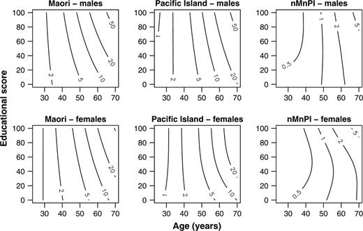
Kaufman et al. show that their method works well for majority ethnic groups. They work with 27 income categories and with age in 1-year categories. With our data, their method is adequate for the nMnPI majority (figure 1). As an example, the 1 percent mortality rate occurs at a younger age for the Maori relative to the nMnPI majority, with Pacific Islanders intermediate. In each ethnic group, this rate occurs at a younger age in males than in females. A protective effect of education is seen in the nMnPI majority for both genders between the ages of 30 and 40 years. At this point, shifting from no education to a secondary school qualification delays the increase in mortality with age by about 10 years.
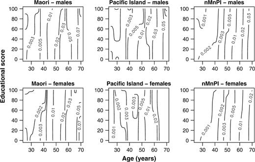
Mortality rate contours using kernel regression, New Zealand, 1996–1999. nMnPI, non-Maori, non-Pacific Island majority.
However, even in the nMnPI majority, kernel regression leads to contours that change in a stepwise fashion rather than smoothly between education categories (figure 1). Kernel regression is essentially a weighted moving average estimating a local constant and, at boundaries in the data, the kernel is asymmetric, and consequently estimates are biased (14). These boundary effects can be mitigated by the use of smoothing methods that estimate a local line or curve, because these provide a more accurate estimate across or into regions where there are no data (14).
As a consequence of equations 2 and 3, the spline is a series of cubic polynomial curves; these curves join at knots, and the knots are constructed so that the “join” is smooth. Fitting the spline requires estimates of the four coefficients that describe each cubic polynomial (15). A full thin-plate spline is a multivariate generalization of this smoothing spline (15), and a thin-plate regression spline is an approximation of the full thin-plate spline; the approximation is quicker to fit and more stable (16, 17). With a bivariate thin-plate regression spline for age and educational score (figure 2), the boundary effects disappear, although the contours for “Pacific Island–males” are clearly unrealistic.
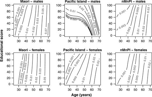
Mortality rate contours using a bivariate thin-plate regression spline, New Zealand, 1996–1999. nMnPI, non-Maori, non-Pacific Island majority.
The generalized additive model is a useful framework for adding and subtracting model structure, following a strategy of adding just enough structure to gain a sensible picture. We could, for example, construct three generalized additive models, one for each ethnic group, with each generalized additive model having an additive difference between male and female in the form of the bivariate spline for age and educational score. However, with our data, we can still produce sensible contour plots even if we smooth each combination of gender and ethnicity separately.
It is reasonable to view death as random and therefore a Poisson process (20). We expect variation in mortality rates between cells of the cross-classification because of both observed and unobserved covariates (20). This suggests that, for each combination of gender and ethnicity, the number of deaths will follow an “overdispersed” Poisson distribution, where the variance in the number of deaths is approximately some multiple of the Poisson mean (21, p. 199) and where the Poisson mean is some unspecified function of age and education. We also expect that the number of deaths will be directly proportional to the person-years at risk. We choose a log-link function, so that the expected number of deaths must be greater than zero. The Poisson generalized additive model that meets these specifications is equivalent to smoothing the mortality rate on a log scale. For each combination of gender and ethnicity, we smooth the mortality rate on a log scale across the dimensions of age and education using a bivariate thin-plate regression spline (figure 3).
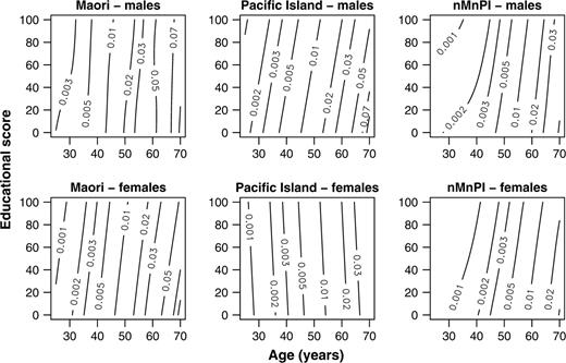
Mortality rate contours using Poisson generalized additive models with smoothing by a bivariate thin-plate regression spline, New Zealand, 1996–1999. nMnPI, non-Maori, non-Pacific Island majority.
Up to this point, we apply the same relative scale between age and education as used by Kaufman et al. However, we do not need to assume a relative scale if we use a bivariate tensor-product spline, a bivariate spline formed from the tensor product (a type of vector multiplication (22)) of univariate spline smoothing in each dimension (23–25). The default univariate spline has five knots, but we set the number of knots for the education dimension to three to ensure at least a degree of smoothing (figure 4).
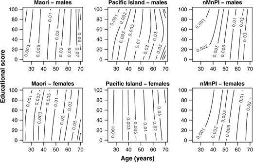
Mortality rate contours using Poisson generalized additive models with smoothing by a bivariate tensor-product spline with knot constraints, New Zealand, 1996–1999. nMnPI, non-Maori, non-Pacific Island majority.
In summary, we suggest three improvements to the smoothing proposed by Kaufman et al. These improvements should give sensible contour plots even when the data are coarsely cross-classified and highly variable. We replace kernel smoothing (figure 1) with spline smoothing (figure 2), smooth the mortality rate on a log scale rather than on a linear scale (figure 3), and use a bivariate spline that is appropriate when variables are measured in different units (figure 4).
For data of this sort, the second step in a conventional analysis might be model building and statistical inference using Poisson regression (9). As an example, at the end of the next section, we consider the hypothesis that the protective effect of education differs between ethnic groups.
HIERARCHICAL BAYESIAN POISSON REGRESSION
If the posterior estimate of ζ is large, this implies strong support for the prior covariate structure. There is then little variance
Having read the analysis by Kaufman et al. (3), we consider the following prior structure for our data: mortality depends on gender, on age but with a different association for different ethnic groups, and on education but with an association that varies with ethnic group and with age. This structure implies a log-linear model for the expected mortality rate (equation 7), with terms for age, sex, Maori ethnicity, Pacific Island ethnicity, educational score, and interaction terms for age and ethnicity, education and ethnicity, and age and education. With a cell count of 10 deaths, we might be ambivalent about the weight attached to this structure and to the observed rate in a cell. This implies that, in cells with higher expected counts, we would want the observed mortality rate to be given more weight than the prior model, and we would want the reverse in cells with lower expected counts.
These prior considerations lead to posterior estimates of the mortality rate (Web appendix A), which we then smooth using a generalized additive model for each combination of gender and ethnicity (figure 5). Our use of generalized additive models in this context is to interpolate continuous age by education surfaces at points where no observation was made, because these surfaces are easier to interpret than a table of 240 cells. Gelman (30) suggests applying the ideas and methods of exploratory data analysis to structures other than raw data, such as plots of parameter inferences; comparing observed (figure 4) and predicted (figure 5) mortality rates may suggest ways in which the fitted model departs from the data. Our approach to the analysis of social variation in health has much in common with the analysis of spatial variation in health (31, 32).

Posterior point estimate contours using gamma generalized additive models with smoothing by a bivariate tensor-product spline with knot constraints, New Zealand, 1996–1999. nMnPI, non-Maori, non-Pacific Island majority.
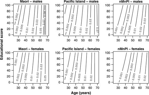
Because the marginal posterior distribution for the mortality rate λi is approximately gamma (26), we smooth these using a gamma generalized additive model with a log link (figure 5). In the same way, we also smooth the widths of the 95 percent credible intervals (Web appendix A; figure 6). The shrinkages Bi are distributed approximately beta and estimated as ai/(ai + bi), where ai and bi are estimates in each cell of the beta distribution parameters (26). The beta distribution does not belong to the exponential family of distributions and so cannot be fit as a generalized additive model. Instead, we smooth ai “successes” in (ai + bi) “trials” as an “overdispersed” binomial generalized additive model with a logit link (figure 7), so that the first and second moments of our generalized additive model are the same as those of the beta distribution (33, 34).
Ninety-five percent credible interval width contours (× 103) using gamma generalized additive models with smoothing by a bivariate tensor-product spline with knot constraints, New Zealand, 1996–1999. nMnPI, non-Maori, non-Pacific Island majority.
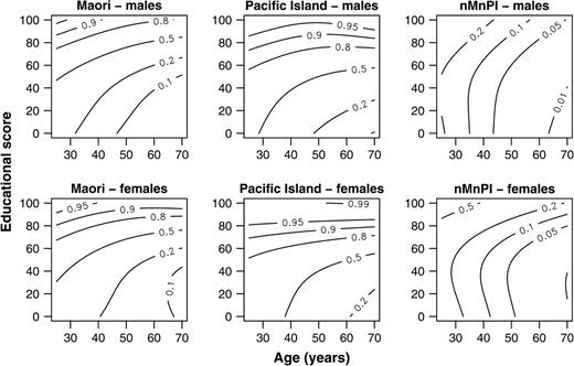
Shrinkage contours using binomial generalized additive models with smoothing by a bivariate tensor-product spline with knot constraints, New Zealand, 1996–1999. nMnPI, non-Maori, non-Pacific Island majority.
To summarize our Bayesian approach, our posterior point estimates of the mortality rate λi (figure 5) are similar to those suggested by exploratory data analysis (figure 4). Of course, exploratory data analysis by itself does not allow a formal comparison of the differences (e.g., between ethnic groups); for this, we need to consider the variance in estimates. The marginal posterior distribution for the λi is approximately gamma with a variance that depends on the posterior mean rate and on the person-years at risk (26). Therefore, credible intervals become wider with age (figure 6), because the mortality rate increases with age. Credible intervals are also wider at higher educational scores, where there are fewer person-years at risk, and for this reason, they are much wider for the two minorities than for the nMnPI majority. Shrinkages show that our prior structure has a strong influence on posterior estimates for both minorities in the region of higher educational scores and younger ages (figure 7), with values in this region close to the maximum value of one.
Posterior estimates of β parameters are often of interest. We consider the hypothesis that the protective effect of education differs between ethnic groups. Using the prior structure previously described and with age centered at 50 years, we find that education appears to have a protective effect such that, in the nMnPI majority, the expected mortality rate at an educational score of zero is 2.35 (95 percent credible interval (CI): 1.95, 2.83) times the expected mortality rate at a score of 100. However, for Maori and Pacific Islanders, the expected mortality rates at a score of zero are only 1.54 (95 percent CI: 1.19, 2.00) and 1.37 (95 percent CI: 0.96, 1.95) times the respective rates at a score of 100.
Credible intervals for the hierarchical Poisson model are wider than confidence intervals for the equivalent conventional Poisson model (table 1). The hierarchical model assesses support for a prior Poisson regression model, so its credible intervals reflect both parameter uncertainty and uncertainty about this prior model. The conventional confidence interval is a conditional inference: It assumes that the fitted Poisson model is correct. This is unrealistic, so estimates from a hierarchical model are typically more accurate—with a lower mean squared error (35, 36)—than those from a conventional model. Here, the conventional model leads to contours without the well-defined curvature in the nMnPI majority that suggests that a secondary school qualification has a strong protective effect (figure 8). This curvature remains in the hierarchical Poisson model (figure 5), even when this conventional model is used as its prior structure, because there is strong support from the data for this curvature and therefore little shrinkage towards the prior structure in this region of the data (figure 7). This curvature suggests that the association among mortality, age, and education is more complex than we anticipated.
Point estimate contours for conventional Poisson regression using Poisson generalized additive models with smoothing by a bivariate tensor-product spline with knot constraints, New Zealand, 1996–1999. nMnPI, non-Maori, non-Pacific Island majority.
Mortality rate for males and females aged 50 years who had an educational score of zero as a multiple of their mortality rate with a score of 100, New Zealand, 1996–1999
Ethnic group | Hierarchical Poisson model | Conventional Poisson model | ||||
|---|---|---|---|---|---|---|
| Mortality rate ratio | 95% credible interval | Mortality rate ratio | 95% confidence interval | |||
| Non-Maori, non-Pacific Island majority | 2.35 | 1.95, 2.83 | 2.16 | 2.04, 2.30 | ||
| Maori | 1.54 | 1.19, 2.00 | 1.53 | 1.34, 1.75 | ||
| Pacific Island | 1.37 | 0.96, 1.95 | 1.47 | 1.14, 1.91 | ||
DISCUSSION
Spline smoothing is likely to give a clearer exploratory data analysis than is kernel smoothing if data are coarsely cross-classified and highly variable within some cells of that cross-classification. The generalized additive model is a useful framework for adding and subtracting model structure following a strategy of adding just enough structure to gain a clear picture. With these tools, the conventional approach—exploratory data analysis followed by modeling and statistical inference—is possible with mortality data from a mixture of majority and minority ethnic groups.
In hierarchical Bayesian Poisson regression, we add model structure by specifying a prior covariate structure. However, both the amount of local information and the overall fit of the prior structure determine the degree to which this prior structure influences posterior estimates of the mortality rate. Markov chain Monte Carlo methods can be used to fit a hierarchical Poisson regression model. However, the method described by Christiansen and Morris is much quicker, so that it is easy to carry out sensitivity analyses using other prior covariate structures or with a different level of confidence (d0) in a given prior structure.
Conventional statistical inference, at least in theory, considers support for hypotheses proposed a priori, rather than for those suggested by exploratory data analysis. In practice, “the best analyses are those that combine both, flagrantly moving easily from ideas the investigator initially proposed to ideas suggested by the data” (37, p. 780). By comparing observed and predicted patterns of mortality, the investigator can identify a variety of models that appear to be consistent with the data (3). However, the investigator may be mislead into reporting false positive results by chance variation in the data (38). The advantage of the hierarchical Bayesian analysis is that its statistical inference is not conditional on specifying the correct Poisson regression model; rather, its intervals reflect both parameter uncertainty and uncertainty about a Poisson regression model proposed a priori. In addition, prior information about the likely direction and magnitude of covariate effects can be incorporated into a hierarchical model by using an informative prior at the highest level of the model (Web appendix B). When the prior evidence for a hypothesis is strong, a positive study is more likely to be a true positive. “The mistake is to confuse an increment in support from a positive study with cumulatively strong support for the hypothesis” (39, p. 958). Focusing on cumulative support for a hypothesis is the key to avoiding spurious findings in epidemiology.
SOFTWARE
All analyses and plots use the R system for statistical computation and graphics version 1.9.1 (40). Generalized additive models were fit with an add-on package, mgcv version 1.1–5. Both R and mgcv are available from the Comprehensive R Archive Network website (http://cran.R-project.org/); further information on mgcv is available from its author, Simon Wood (http://www.maths.bath.ac.uk/∼sw283/). The hierarchical Poisson regression model of Christiansen and Morris was fit by use of their Splus code (PRIMM), available from the “Statlib” website (http://lib.stat.cmu.edu/S/). Minor changes are needed to make this code run within the R system.
SUMMARY OF STATISTICS NEW ZEALAND SECURITY STATEMENT
The full security statement is published at http://www.wnmeds.ac.nz/nzcms-info.html.
The New Zealand Census-Mortality Study is a study of the relation between socioeconomic factors and mortality in New Zealand, based on the integration of anonymous population census data from Statistics New Zealand and mortality data from the New Zealand Health Information Service. The project was approved by Statistics New Zealand as a Data Laboratory project under the Microdata Access Protocols in 1997. The data sets created by the integration process are covered by the Statistics Act and can be used for statistical purposes only. Only approved researchers who have signed Statistics New Zealand's declaration of secrecy can access the integrated data in the Data Laboratory. For further information about confidentiality matters in regard to this study, please contact Statistics New Zealand.
This project was supported by a University of Otago research grant.
The authors thank June Atkinson and Richard Penny for sharing their knowledge of the data used in this project and Simon Wood for his help with mgcv.
Conflict of interest: none declared.
References
Smith GD. Learning to live with complexity: ethnicity, socioeconomic position, and health in Britain and the United States.
Nazroo JY. The structuring of ethnic inequalities in health: economic position, racial discrimination, and racism.
Kaufman JS, Long AE, Liao Y, et al. The relation between income and mortality in U.S. blacks and whites.
Greenland S, Robins JM. Identifiability, exchangeability, and epidemiological confounding.
Blakely T, Woodward A, Salmond C. Anonymous linkage of New Zealand mortality and census data.
Hill S, Atkinson J, Blakely T. Anonymous record linkage of census and mortality records: 1981, 1986, 1991, 1996 census cohorts. Wellington, New Zealand: Department of Public Health, Wellington School of Medicine and Health Sciences, University of Otago,
Blakely T, Robson B, Atkinson J, et al. Unlocking the numerator-denominator bias. I. Adjustments ratios by ethnicity for 1991–94 mortality data. The New Zealand Census-Mortality Study.
Blakely T, Kawachi I, Atkinson J, et al. Income and mortality: the shape of the association and confounding New Zealand Census-Mortality Study, 1981–1999.
Michels P. Asymmetric kernel functions in nonparametric regression: analysis and prediction.
Silverman BW. Some aspects of the spline smoothing approach to nonparametric regression curve fitting.
Hastie T, Tibshirani R. Generalized additive models; some applications.
Wood SN, Augustin NH. GAMs with integrated model selection using penalized regression splines and applications to environmental modelling.
Brillinger DR. The natural variability of vital rates and associated statistics.
McCullagh P, Nelder JA. Generalized linear models. 2nd ed. London, United Kingdom: Chapman and Hall,
Wood SN. Low rank scale invariant tensor product smooths for generalized additive mixed models. Glasgow, Scotland: Department of Statistics, University of Glasgow,
Christiansen CL, Morris CN. Hierarchical Poisson regression modeling.
Albert JH. Bayesian estimation of Poisson means using a hierarchical log-linear model. In: DeGroot MH, Lindley DV, Smith AFM, et al, eds. Bayesian statistics 3: proceedings of the Third Valencia International Meeting, June 1–5, 1987. Oxford, United Kingdom: Oxford University Press,
Albert JH. Computational methods using a Bayesian hierarchical generalized linear model.
Pascutto C, Wakefield JC, Best NG, et al. Statistical issues in the analysis of disease mapping data.
Kieschnick R, McCullough BD. Regression analysis of variates observed on (0,1): percentages, proportions, and fractions.
Papke LE, Wooldridge JM. Econometric methods for fractional response variables with an application to 401(k) plan participation rates.
Hertz-Picciotto I. What you should have learned about epidemiologic data analysis.
Savitz DA. Commentary: prior specification of hypotheses: cause or just a correlate of informative studies?

