Piecewise linear approximation of protein structures using the principle of minimum message length

Abstract

1 INTRODUCTION

With the rapid growth in the corpus of known structures, concise representations are increasingly preferred to inspect and analyze protein folding patterns (Abagyan and Maiorov, 1988; Lesk, 1995; Richardson, 1981; Taylor et al., 1983). At the core of this simplification is the idea that proteins contain repetitive substructural elements and that the essence of a fold lies in the assembly and interaction of these elements (Kamat and Lesk, 2007; Konagurthu and Lesk, 2010; Lesk and Chothia, 1980; Lesk, 1995).

The appearance of some of these elements arises from the periodicity in the patterns of hydrogen bonds between backbone nitrogen and carbonyl groups along the protein polypeptide chain. Among the standard secondary structure definitions are: helix (α-helix, π-helix and 3₁₀-helix) and strand of sheet (Edsall et al., 1966). Ideally, the spatial trace of α-Carbon (C_α) atoms of standard secondary structure show a linear trend allowing them to be abstracted using vectors or line segments, without much loss of structural information about the fold. The common practice is to fit an axis to a helix and a least-square line to C_α or main chain atoms of strands of sheet (Chothia et al., 1981; Lesk, 1995).

Replacement of secondary structural elements with line segments is therefore one of the common methods to abstract protein structures and construct concise representation of their folding patterns. The number of standard secondary structural elements observed in a protein is typically an order of magnitude smaller than the number of residues in a chain. Therefore methods that utilize concise representations clearly benefit from a massive space and computational saving, especially when comparing and analyzing structures on a large scale (Abagyan and Maiorov, 1988; Konagurthu et al., 2008; Mizuguchi and Go, 1995; Shi et al., 2007).

Methods that abstract protein structure at the level of secondary structure generally rely on external programs that can automatically assign secondary structures to coordinate data. However, accurate identification and assignment of secondary structure is an inexact process (Cuff and Barton, 1999). Although definitions based on hydrogen bonding provides some rigor in assigning secondary structure, the standard definition of what constitutes a hydrogen bond is based on the notion of bond energy whose measurement can be imprecise and acutely sensitive even to small differences in the position of nitrogen and carbonyl atoms, especially the carbonyl oxygen positions. Two popular programs that use hydrogen bonding as a basis for assignment of secondary structure are DSSP (Kabsch and Sander, 1983) and STRIDE (Frishman and Argos, 1995).

On the other hand, secondary structure can be defined using geometric features such as distances and dihedral angles of C_α atoms along the backbone in addition to other local structural features. In fact, there is a direct correlation between patterns of hydrogen bonding and the geometry that arise out of them. However, secondary structural elements can deviate substantially from ideal geometry, therefore posing severe challenges to detect such elements using geometric features alone. Among the methods that rely primarily on geometry to assign secondary structure are (Dupuis et al., 2004; Labesse et al., 1997; Levitt and Greer, 1977; Majumdar et al., 2005; Richards and Kundrot, 1988; Sklenar et al., 1989; Srinivasan and Rose, 1999; Taylor, 2001). (See (Majumdar et al., 2005) for details of popular programs that assign secondary structural elements.)

We note that previous comparative studies have highlighted the difficulties of existing programs to assign consistently secondary structure to coordinate data and have proposed using a ‘consensus’ definition—secondary structure assignment that is at the intersection of all the methods—to arrive at a reliable simplification of protein structures (Colloc'h et al., 1993; Cuff and Barton, 1999).

The main goal for abstracting protein structures must be to achieve maximal economy of description with minimal loss of structural information (Taylor, 2001). However, simplifying structures at the level of standard secondary structure is lossy because the loop regions are ignored. Therefore, a reliable method that achieves the above goal and that is tolerant to measurement error and noise is preferred. Even better would be a method entirely independent of preconceived notions of what substructures are being sought.

Here, we describe a method that generates a principled abstractions of protein structures. Our method uses the rigorous statistical framework of minimum message length (MML). In fact, the realization of the goal to maximize economy and minimize loss of information fits squarely into the MML criterion, making it extremely well-suited for this specific problem. In this work, we treat a protein as an ordered list of C_α coordinates. Our method uses an information-theoretic approach to explain as a line segment the points between any pair of residues in the structure. Each such explanation is encoded in a certain number of bits (or code length). Using these code lengths, a globally optimal explanation is computed which minimizes the total encoded (message) length of the given coordinate data. The code lengths contributing to this minimum message length result in the best piecewise linear approximation of the structure. In a stark contrast to the existing methods, our method is completely free of parameters and thresholds. We emphasize that our method is not a method for delineating secondary structures. However, as expected from such a method, our results show that the line segments generated by this method correspond well with standard secondary structures of proteins.

We note that this article generalizes to three dimensions the work of Banerjee et al. (1996), who described a polygonal approximation method on general two dimensional sequence of points.¹ Indeed, it can be shown that our method described in this paper can be generalized to arbitrary dimensions and other types of structural data (over and beyond proteins). We have attempted to keep the notations in this paper consistent with those described in the work of Banerjee et al. (1996) for the convenience of the reader.

Section 2 briefly summarizes the MML framework, followed by Sections 3–6 which describe the mechanics of our approach. Section 7 presents an analysis of the results of our method over a large number of protein structures.

2 THE MINIMUM MESSAGE LENGTH FRAMEWORK

Wallace and Boulton (1968) first proposed the theory of MML, where given a set of competing hypotheses (or models) that can explain some observed data, the MML criterion provides a statistically rigorous framework for selecting the best hypothesis to describe the data. In many ways, MML is a formal information-theoretic realization of the principle of Occam's razor.

Assume there are some observed data D and some hypothesis H that explains the data. From Bayes's theorem we get

where p(H&D) is the joint probability of data D and the hypothesis H, p(H) is the prior probability of hypothesis H, p(D) is the prior probability of data D, p(H|D) is the posterior probability of H given D, and p(D|H) is the likelihood.

MML applies the remarkable result from Shannon's ‘Mathematical Theory of Communication’ (Shannon, 1948) that, given an event E with a probability p(E), the message length, l(E) for an optimal code is given by l(E)=−log₂(p(E)) bits. Carrying this insight to the Bayes's theorem, we get the following relationship between conditional probabilities in terms of optimal message lengths.

The essence of inductive inference is to fit a model to a mass of observed data. For such an approach it is the hypothesis H with the largest posterior probability p(H|D) that is often preferred. Among the terms in the above equation, p(H) (and hence l(H)) can usually be estimated well for some reasonable prior on hypotheses. At the same time, the likelihood p(D|H) can also be estimated. But to estimate the posterior probability distribution p(H|D), the prior of observed data p(D) will be needed. Estimating p(D) can be problematic and even impractical. However, for two competing hypotheses, H and H^′ we; have

thereby eliminating the necessity to estimate p(D) completely when comparing hypotheses.

MML is best understood through a communication process where a transmitter and a receiver are connected through one of Shannon's communication channels. The objective is that a transmitter must send some data D to the receiver. The transmitter and receiver must have previously agreed on a set of rules (that is, a code book) of communication using common knowledge and prior expectations. If the transmitter can find a good hypothesis, H*, to fit the data, (s)he will be able to transmit the data economically.

In MML, an explanation of the data comes as a two part message: Such a message paradigm ensures complete transparency in communication. That is, any information that is not common knowledge cannot be included except as a part of the message sent by the transmitter. Otherwise, the message sent will be indecipherable by the receiver. There can be no hidden parameters in this framework of communication. In fact, this issue extends to stating and inferring real-valued parameters to an ‘appropriate’ level of precision, which is pertinent to the current problem on hand.

1. transmit the hypothesis H* taking l(H*) bits, and

2. transmit the observed data D given H* taking l(D|H*) bits.

The MML framework additionally offers ‘safety’ in that if an inefficient code is used to encode a message, it can only make the hypothesis look less attractive than otherwise. Note that MML yields a natural hypothesis test: the null-model corresponds to transmitting the data raw. If a stated hypothesis takes longer than what is required by a null-model, then clearly such an hypothesis is unacceptable. A more complex hypothesis fits the data better than a simpler model, in general. We see that MML encoding gives a trade-off between hypothesis complexity (l(H)), and its goodness of fit to the data (l(D|H)). Therefore, MML criterion formally justifies and realises Occam's razor.

An important aspect of MML framework is that it is tolerant to measurement accuracy and noise in the underlying data. For a justification of this and a comprehensive study of the principle of MML, refer (Wallace, 2005).

3 FORMULATING THE PROBLEM USING MINIMUM MESSAGE LENGTH

A protein 𝒫={P₁,···,P_n} is a sequence² of n three-dimensional points corresponding to the coordinates (in ℝ³) of C_α atoms along the protein backbone, from its N- to C- terminus.³

Define a piecewise linear approximation of 𝒫 as a subsequence of k≤n points from 𝒫 of the form 𝒬={Q₁≡P_i1,…,Q_k≡P_ik} such that 1=i₁<···<i_k=n, and the first and last points of 𝒬 are the same as the first and last points of 𝒫 (i.e. Q₁=P₁ and Q_k=P_n).

Given some subsequence 𝒬 of sequence of points 𝒫, the protein can be approximated (or simplified) using line segments drawn between every successive pair of points in the subsequence, Q_r^′ and Q_r^′+1, 1≤r^′<k. We will use the term delineation to describe this piecewise linear approximation. Further, we will use the term endpoint to describe any point in 𝒬. This is because any pair of consecutive points, Q_r^′≡P_ir^′ and Q_r^′+1≡P_ir^′+1, form endpoints for abstracting the points between P_ir^′ and P_ir^′+1 (inclusive) in the protein with a line segment. Note that a subsequence 𝒬 with k endpoints yields a delineation containing k−1 line segments between successive endpoints.

The goal this article is to find the best delineation of a given set of coordinate data, where the objective to select the best comes from defining the problem using the minimum message length criterion. Consistent to the communication process described in Section 2, the transmitter explains the data in 𝒫 with a hypothesis 𝒬 and sends it as a message whose code length is globally minimum over all possible hypotheses. Receiver will then able to infer the entire data 𝒫 from the received message to a reasonable level of precision using the general rules they have agreed upon as a part of the code book.

For the problem of delineating a structure from coordinate data, the transmitter will send the following two part message (refer Section 2): Therefore, as a part of the codebook, the transmitter and receiver must have agreed upon the encoding of the endpoints in 𝒬 and the encoding of deviations of points 𝒫−𝒬 explained by line segments between successive endpoints in 𝒬. Since the coordinate data of proteins is available at some fixed precision, the transmitter and receiver agree on the specific precision at which the data should be sent. We emphasize that the encoding of the above should allow the receiver to decode the message to the agreed precision.

1. The first part is the subsequence of points 𝒬 which denotes the delineation of 𝒫. This is equivalent to transmitting the hypothesis 𝒬 in l(𝒬) bits.

2. The second part will contain the remainder of points in 𝒫 (that is, 𝒫−𝒬) that weren't sent in the first part. In other words, these are the points in 𝒫 that are between the endpoints stated in 𝒬. The statement of these points will be encoded as spatial deviations with respect to the line segments between endpoints. This is equivalent to transmitting the observed data 𝒫 given the hypothesis 𝒬 over l(𝒫|𝒬) bits.

4 CODE LENGTH TO STATE THE DELINEATION AND DATA UNDER MML CRITERION

In this section, we will discuss the statement and transmission of the two part message described in Section 3.

4.1 Encoding the first part of the message

The first part pertains to the transmission of the delineation 𝒬 containing k endpoints. The transmitter must therefore state the number of points k. There are several optimal universal prefix codes available to encode integers. Here, we use an asymptotically optimal Elias omega code which encodes the integral value k in log*k bits⁴ (Elias, 1975).

Next, the coordinates of all endpoints are to be encoded. Each endpoint is a set of three real numbers of the form (x,y,z). Published protein coordinate data contain three putatively significant figures after the decimal point, in Angstrom Å units. The transmitter can scale this data to one decimal precision and treat the coordinates as integers. Now, an optimal code to send these coordinates is for the transmitter to first send the coordinates of a bounding rectangular box, (x_min,y_min,z_min) and (x_max,y_max,z_max) over all possible values of x,y and z in the given data. Once this bounding box is specified, any (x,y,z) coordinates within the box can be coded in log(x_max−x_min)+log(y_max−y_min)+log(z_max−z_min)=log((x_max−x_min)(y_max−y_min)(z_max−z_min))=log V bits, where V is the volume of the bounding rectangular box. It follows from here that all the k endpoints in 𝒬 can be stated in klog V bits.⁵

Therefore, the message length to state the first part of the transmission requires log*k+klog V bits.

4.2 Encoding the second part of the message

In the second part, the transmitter has to encode the data, 𝒫−𝒬, between endpoints stated in the first part of the message. For a successive pair of endpoints (Q_r^′≡P_i,Q_r^′+1≡P_j), 1≤i<j≤n, 1≤r^′≤k in 𝒬, there are j−i−1 intermediate points between P_i and P_j in 𝒫. In this work, these intermediate data points will be treated as noisy samples and will be stated as a set of spatial deviations with respect to the line segment between P_i and P_j.

If such a scheme is used to communicate the second part of the message, for each line segment in 𝒬 between successive endpoints, the second part of the message will encode the following information:

1. the number of points explained by the line segment.

2. three spatial deviations for each intermediate point with respect to the line that will allow the receiver to recover the original location of the intermediate point up to a reasonable approximation.

3. the parameters of the probability distribution associated with each of the three sets of spatial deviations, over all intermediate points.

To explain the encoding of this part more clearly, consider Fig. 1. Let L_ij denote the line segment between two successive endpoints in 𝒬, Q_r^′≡P_i and Q_r^′+1≡P_j. This line will be used to explain the intermediate points P_i+1···P_j−1∈𝒫. For any intermediate point P_r, i+1≤r≤j−1, define three spatial deviations Δ s_r, t_r and u_r. In the reverse order, u_r is the signed distance of P_r to the plane defined by vectors P_j−P_i and z-axis. To define t_r, first project P_r to the plane defined above. Call this projection point ⁠. Given this projection, t_r is the signed perpendicular distance of to the line L_ij. Finally, the deviation Δs_r is the (unsigned) lateral distance along the line L_ij between points of projection of and onto the line (Fig. 1). (Refer the supplementary note containing a discussion on these deviations under arbitrary rotation of the coordinates.) Note that once the endpoints P_i and P_j are specified, and given the sets of spatial deviations Δ s_r's, t_r's and u_r's for the intermediate points P_r, ∀i<r<j, the receiver can entirely recover the coordinates of all intermediate points.

Fig. 1.

Open in new tabDownload slide

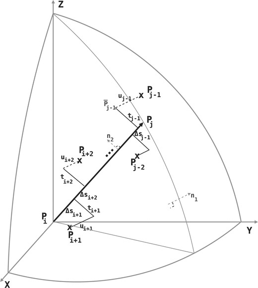
Deviations Δs,t and u of intermediate points P_i+1··· P_j−1 to a line segment between two endpoints P_i and P_j. (Refer main text.)

In this work, we assume the three spatial deviations Δ s's, t's and u's of the intermediate points to be independent and normally distributed. Individual variables of each distribution are considered independent and random. (See supplementary note for a discussion on these assumptions.) Given these assumptions we have three distributions of the form: Δs~𝒩(μ_Δs,σ²_Δs), t~𝒩(μ_t,σ²_t), and u~ 𝒩(μ_u,σ²_u), where μ and σ² are the mean and variance of the respective normal distributions. For the structural coordinate data, we assume that the mean of the distributions of t's and u's is zero: t~𝒩(0, σ²_t), and u~𝒩(0, σ²_u). Therefore, to communicate the three distribution, the transmitter has to state the following four parameters: (μ_Δs, σ²_Δs, σ²_t, σ²_u).

Consider the calculations of these parameters. For the line L_ij, there are j−i−1 intermediate points. Represent this quantity by the variable m_ij. Then

where D_ij is the Euclidean distance between P_i and P_j. Note that once the endpoints are transmitted (see Section 4.1), the receiver can deduce the value of μ_Δs requiring no explicit statement for this parameter in the message. This reduces the number of parameters to be stated from four to three: (σ²_Δs, σ²_t, σ²_u).

We will now compute the code lengths to state the variance of three normal distributions. Variance for a Gaussian distribution is simply ‘mean squared minus squared mean’:

Similarly, we have and ⁠, since μ_t=μ_u=0. We note that the code length for each parameter varies with bits. [See Chapter 5 of (Wallace, 2005)].

With the parameters of the distributions encoded, we will now compute the code lengths required to state the individual values of Δs's. Since we have assumed that the distribution is a Gaussian, the probability distribution of a random variable Δs_r with parameters μ_Δs and σ_Δs² is given by:

Since we assumed that variables are independent, we have

This implies,

Therefore, using Shannon's insight, the optimal code length to describe the entire sets of individual deviations of Δs's for a line L_ij will require −log(p(Δs_i+1,…,Δs_j−1|𝒩(μ_Δs, σ²_Δs))) bits.

Following a similar expansion, we can show that the code lengths for the deviation t_r's and u_r's are and ⁠, respectively.

So far in this second part, we have computed the code lengths required to state intermediate points explained by the line L_ij. Note that a delineation of a structure containing k endpoints defines k−1 such line segments. For convenience in notation, assume the endpoints of each line segment is of the form (P_ir,P_jr), 1≤r<k. (In practice, for a delineation, P_ir of the r-th line segment is equivalent to P_jr−1 of (r−1)th line segment.) Then the total code length of the second part is the sum of the following terms:

1. ∑_r=1^k−1log* m^r_ij, where m^r_ij=j_r−i_r−1, representing the total code length to encode the number of intermediate points described by all line segments in the delineation put together.

2. bits to encode the parameters (three per line segment) corresponding to the distribution of spatial deviations for all lines.

3. bits to encode Δs_r's over all line segments

4. bits to encode t_r's over all line segments

5. bits to encode u_r's over all line segments

4.3 Problem statement

Given a delineation 𝒬 (hypothesis) of coordinates 𝒫 (data), denote the total message length required to explain the data by the hypothesis as ℋ(𝒬). Combining the code lengths to state the two part message described in Sections 4.1 and 4.2, the total message length is:

(1)

Since log*k≪klog V, the transmitter can ignore stating that term in the code length. Assume

(2)

ℋ^r_ij denotes the component code length to express each line segment L^r_ij with endpoints P_i^r and P_j^r, given a delineation 𝒬. This implies This allows us to formally define the delineation problem as follows:

The problem:

Given 𝒫 containing a sequence of n points, find a subsequence 𝒬∈𝒫 containing k≤n points such that the total message length to explain 𝒫 with 𝒬, ⁠, is globally minimum.

5 FINDING THE OPTIMAL DELINEATION

This section will describe the procedure to compute the optimal delineation 𝒬* for a given coordinate data. Broadly, the search for the optimal delineation has two steps.

Potentially every pair of points P_i and P_j, 1≤i<j≤n can be a part of the delineation in 𝒬*. (We note here that the segments in the delineation must not overlap, except for successive regions, and those only at their endpoints.) Therefore, we will first build a matrix ℋ=(ℋ_ij)_1≤i<j≤n of code lengths for all possible pairs of points in 𝒫.

Then, the matrix ℋ will be used to find a subsequence of points 𝒬* such that the total code length ℋ(𝒬*) of the delineation is minimized, using a one-dimensional dynamic program.

5.1 Computation of code length over all possible segments

Equation (2) expresses the message length ℋ_ij required to describe any line segment L_ij between two points P_i and P_j. We will examine the complexity of computing each of the components that constitute Equation (2).

For the n points in 𝒫, there are possible line segments. The log V term in Equation (2) is constant across all possible segments and is computed once while reading the data points of 𝒫. Next, for each line segment, there are three parameters whose code lengths depend on the number of points in between the endpoints. This is trivially computed in constant time as j−i−1.

The relatively complex part is to compute the code lengths of the spatial deviations of the line, Δ s's t's and u's. Each of these three deviations have code lengths that depend on their respective variance, σ²_Δs, σ²_t and σ²_u. While one can compute the variance of each set of deviations from the coordinate data, such a computation is linear in the number of points that each line segment explains. If this näive approach is followed, the computation of ℋ requires O(n³) operations. We will show in the later Section 6 that this is redundant and that the total time required to compute ℋ can be achieved in O(n²) operations, by computing the variances of all three spatial deviations incrementally from previous computations using a set of sufficient statistics. But before that we will describe the method to compute the optimal delineation given the matrix ℋ.

5.2 Optimal delineation as a one-dimensional dynamic program

Dynamic programming is perfectly suited when dealing with problems that contain sequential constraints, where the solutions to the subproblems have a recursive overlapping substructure (Bellman, 1957). The problem statement in Section 4.3 is an ideal candidate for the search strategy of dynamic programming. Since a delineation is a subsequence which preserves the linear ordering of its elements, the optimal delineation of the given data can be derived by computing and memoizing (i.e. caching) the optimal delineation of its subproblems.

We will use the matrix ℋ of code length between all possible endpoints to find the optimal delineation 𝒬* that minimizes ℋ(𝒬*) using a one-dimensional dynamic program.

Let C_i be an array that stores the optimal code length of delineating points P₁,…, P_i, ∀1≤i≤n. The objective is to find the delineation of the given points where C_n is minimum over all possible subsequences of the given points. Therefore, the recurrence relationship of optimal costs using a one-dimensional dynamic program is as follows:

In other words, the optimal code length to delineate the points P₁,…,P_j (1≤j≤n) builds on the optimal code length to delineate from P₁,…,P_i, if and only if the value of C_i plus the code length to state a new line segment ℋ_ij is minimum, over all 1≤i<j.

Using the above relationship, the array C is filled iteratively from 1 to n. Upon completion, the value C_n gives the optimal message length corresponding to the best delineation 𝒬* of 𝒫, where ℋ(𝒬*)≡C_n is globally minimum. The subsequence of endpoints of this optimal delineation can be computed by storing, for each j, the back pointer i<j of the array from which the optimal value C_j was derived. With these back pointers, a simple traceback from C_n (until C₁ is reached) gives the set endpoints (in reverse order) that form the best delineation 𝒬*.

6 EFFICIENT COMPUTATION OF MATRIX ℋ

As mentioned in Section 5.1 the matrix of code lengths ℋ can be computed efficiently in O(n²) operations and this section will show how this can be achieved.

For the matrix ℋ to be computable in O(n²) operations, each element ℋ_ij in the matrix should be computable in constant time. However terms σ^r_Δs², σ^r_t², and σ^r_u² in Equation (2) cannot be computed in constant time. For a line segment L_ij, näively, these three variances take time proportional to the number of points explained by the line to compute, leading to a O(n³) algorithm for computing the matrix ℋ. Below we will show that each of σ^r_Δs², σ^r_t², and σ^r_u² can indeed be computed incrementally and in constant time from previous computations resulting in a O(n²) algorithm.

6.1 Constant-time update of σ²_Δs's

Consider first these notations: for any vector with direction ratios 〈x,y,z〉, let represents the vector norm of ⁠. Let any point P_i∈𝒫 have the direction ratios of the form 〈x_i,y_i,z_i〉.

By the definitions of the spatial deviations in Section 4.2, any Δs_r, 1≤i<r<j≤n is the scalar associated with the projection of the vector (P_r−P_r−1) onto the vector L_ij≡(P_j−P_i). (Refer Fig. 1.) Let represent the direction cosines of the vector L_ij, where ⁠, and ⁠. Then Δs_r is the dot product of (P_r − P_r−1) and ⁠: ⁠. Expanding this we get,

Denoting

(3)

Now, let S_ij^xx, S_ij^yy, S_ij^zz, S_ij^xy, S_ij^yz, S_ij^xz be a set of variables which we will call here sufficient statistics. These variables are of the form: ⁠, where A and B take the values {x,y,z}.

Expressing Equation (3) in terms of the sufficient statistics, we get

(4)

From Equation (4) it can be clearly seen that any S_ij+1 can be updated from S_ij in constant time, using the sufficient statistics. This holds because any S_ij+1^AB=S_ij^AB+(A_j−A_j−1)(B_j−B_j−1), where {A,B}∈{x,y,z}.

Therefore, using the sufficient statistics the computation of σ_Δs for a line segment can be computed incrementally in constant time.

6.2 Constant-time update of σ²_t's

Let be the normal to a plane defined by ⁠, where is the unit vector along z-axis with the direction cosines 〈0,0,1〉. It follows that the direction ratios of are 〈−(y_j−y_i),(x_j−x_i), 0〉.

Define as a vector which is normal to the plane ⁠. The direction ratios of will be: 〈−(x_j−x_i)(z_j−z_i),−(y_j−y_i)(z_j−z_i),(x_j−x_i)²+(y_j−y_i)²〉 Let represent the direction cosines of ⁠, where ⁠, and ⁠.

Then ⁠. (Refer Fig. 1.) This implies

Assume and expanding along the steps we took in the previous section, we get

(5)

where computation of any T_ij+1 can be updated from T_ij in constant time.

6.3 Constant-time update of σ²_u's

We have seen above that ⁠. Let represent the direction cosines of ⁠, where ⁠, and ⁠. (Note ⁠).

Then ⁠. (Refer Fig 1.) Expanding as before we get

(6)

where again the computation of any U_ij+1 can be updated from U_ij in constant time, when sufficient statistics are maintained.

Therefore, the update rules in Equation (4)–(6) allows an efficient computation of the matrix ℋ of code lengths in O(n²) operations.

7 RESULTS

In the previous sections, we have demonstrated an efficient and statistically robust algorithm to simplify a protein structure with piecewise linear segments. We implemented the described algorithm (in C++). Our implementation is available from http://www.csse.monash.edu.au/~karun/pmml/.

We evaluated our method using a non-redundant dataset containing 15 399 protein structures obtained from the protein data bank (Berman et al., 2002). (The non-redundancy here implies that no two structures in this dataset share a sequence identity >65%.) This dataset was culled using the program PISCES (Wang and Dunbrack, 2003). The list of proteins structures in the dataset and the results of their delineation produced by our method can be obtained from the aforementioned link.

Figure 2 gives the distribution of the measure of simplification of structures over the entire dataset. For a structure, the measure of simplification is the ratio of number of line segments identified by the program over the number of residues in the structure. On an average over the entire dataset the delineation size (that is, the number of line segments in the delineation) constitutes 13.85% of the total size of structure (in residues). In addition, the average segment length over the entire dataset is observed to be 8.11 residues. In general, the number of segments is correlated to total size of the protein structure.

Fig. 2.

Open in new tabDownload slide

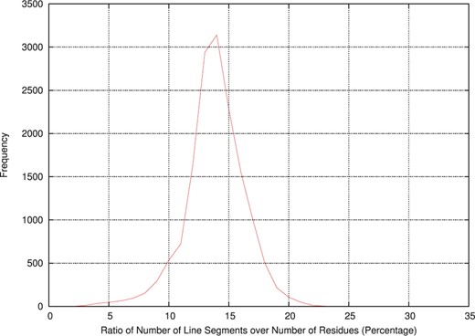
Distribution of ratios of number of line segments over number of residues per structure in the dataset. Ratios are expressed in percentages and rounded to the nearest integral value.

It is of considerable interest to evaluate the agreement of standard secondary structural elements—helices and strands of sheets—with the delineation identified by the program. We note that an ideal delineation of a structure must encompass these elements since they are ideal candidates for approximation with lines or vectors given the linear spatial trend in their geometry. In order to evaluate the agreement, we coarsely classify each segment to one of three secondary structure states: ‘Helix’, ‘Strand’ and ‘Other’. This three-state classification is based on certain geometric characteristics of the segments in the delineation. Specifically, we compute the following geometric profiles for each segment: ‘rise’, ‘pitch’ and backbone dihedral angles ϕ and ψ. The rise (ρ) of the segment with endpoints P_i and P_j is ρ=D_ij/(j−i+1), where D_ij is the Euclidean distance between the endpoints. In other words, the rise gives the average translation of points along the line between endpoints. The rise of a standard secondary structure is directly related to the pitch (p) of the segment. For a substructure with a geometry that repeats itself every n residues, the relationship between rise and pitch is given by p=nρ. Table 1 summarizes the geometric profiles of ideal secondary structures (Taylor, 2001). Inspecting these profiles per segment, a coarse characterisation for each segment in the delineation is achieved.

Examining the coarse segment level assignment for the structures in the dataset, we note that the average length of segments assigned as ‘Helix’ is 13.01 residues while the same for those assigned as ‘Strand’ is 7.33 residues.

To evaluate our coarse assignment, we choose two popular and extensively used secondary structure assignment programs, DSSP (Kabsch and Sander, 1983) and STRIDE (Frishman and Argos, 1995). DSSP and STRIDE assign each residue to one of multiple secondary structural states, including 3₁₀-, α-, π-helices and β-strands of sheet. For the structures in our dataset, we generate the respective secondary structure assignments using DSSP and STRIDE. We note that both these programs assign secondary structure definitions at a residue level, while the coarse assignment for our method described above is at a segment level. Therefore, to enable a comparison between the methods we assign all residues within a segment to the segment level secondary structure state.

Table 2 gives the concordance of Helix⁶ and Strand assignments between DSSP, STRIDE, and our method, PMML.

Although even a coarse segment level assignment by our method produced a satisfactory concordance with DSSP and STRIDE, there is still a disagreement of ~15% between PMML and the other two methods. Inspecting these differences we note that the majority of them came from the terminal parts of the segments delineated by our program. Therefore, we refine the coarse level assignment produced by PMML using the hydrogen bonding patterns of residues within each segment to reassign the secondary structure state at a residue level. We use a simple proximity (of backbone nitrogen and carbonyl groups) and angle (of N, O, C atoms) based computation of hydrogen bonds. Comparing our refined assignments at a residue level with DSSP and STRIDE we notice a substantial improvement in the concordance of helix and stand assignments with DSSP and STRIDE. (See rows 3 and 4 in Table 2.) We emphasize that although PMML can be used to generate protein secondary structure assignments, its real aim is to generate concise representations of structures, irrespective of the nature of the segments of which they are composed. For instance, PMML could be applied to RNA structures without needing any appeal to the types of substructure anticipated.

Manually evaluating the delineation of a large number of structures we notice that although PMML's delineation identifies the regions of helix and strand consistently, there remain small discrepancies in assigning precise beginning and end residues of secondary structure elements as ascertained by an expert. To highlight these differences consider the following example of the delineation produced by PMML. Figure 3 shows the structure of oxidized Clostridium beijerinckii flavodoxin. This protein binds a cofactor, flavin mononucleotide (FMN). Flavodoxin is a small α/β protein, containing a 5-stranded parallel β-sheet (β₁,…,β₅), with two helices packed against each face of the sheet (α_A,α_E and α_C,α_D). There is also a short helix (α_B) located near the N-terminus of the protein. (Fig. 3.) Different segments produced by PMML are shown in different colors. The elements of secondary structure shown as thick ribbons are the secondary structure assignments taken from the structure's wwPDB file (5NLL). Table 3 gives the residue ranges (that is, start and end residues) for each secondary structural element (SSE) of the flavodoxin structure listed in its wwPDB file. The residue ranges of the corresponding segmentation produced by PMML is also presented in the table. Broadly, the program correctly assigns segments to the SSEs. However, minor differences can be observed in the locations of their start and end residues. In most cases, we notice an absolute difference of 1 or 2 residues in the N- or C- terminal regions of these SSEs. The segmentation in the regions around the SSEs α_E, β₂ and β₅ show some discrepancies. The residue range from wwPDB corresponding to α_E was approximated by PMML using 2 segments instead of one. The first segment is composed of roughly one turn of the helix at α_E's N-terminal end. This is understandable as this turn is substantially skewed from the main helical axis and, indeed, there is an interruption in the hydrogen bonding. However, the second segment composed of 11 residues in this region is consistent with the assignment in the wwPDB file. In the case of β₂, the start location identified by PMML precedes the start location identfied in the wwPDB file by four residues. On inspecting the flavodoxin structure, there appears to be a backbone hydrogen bond between the carbonyl group of residue Asp29 and the nitrogen of Met1 (of strand β₁), so the β₂ strand may well start at residue Lys28 or Asp29. Similarly, for β₅, the start location of the segment from PMML was identified to be three residues before the location identified in the wwPDB file, and inspecting the structure, we note the β−bulge in strand β₅, and hydrogen bonds between atoms 80O···109N and 82N···109O; assignment of the start of the strand β₅ to residue 109 is not indefensible.

Fig. 3.

Open in new tabDownload slide

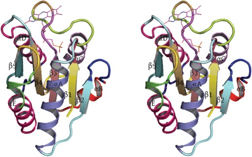
Wall-eye stereo image of 1.8 Å crystal structure of oxidized Clostridium beijerinckii flavodoxin. Each delineated segment produced by PMML is shown in a different color. The elements of secondary structures, of helices and strands of sheet, were derived from the wwPDB file, 5NLL, and are shown in this figure as thick ribbons. The labels of various secondary structures are also shown. The bound FMN co-factor is shown at the top of the structure as thin lines.

8 CONCLUSION

We have presented a novel and efficient method to delineate protein structures using the MML framework; MML is tolerant to measurement error and other inaccuracies. The model used in this work is independent of preconceived notions of what substructures are being sought to simplify the observed coordinate data. Our method maximizes the economy of representation while minimizing the loss of information, taking into account even the loop regions of proteins. Analysis of the delineations of a large number of protein structures suggests that the method is consistent in, among others, delineating standard secondary structures. The concise representations produced by this method have a potential use for rapid and accurate structure comparison and lookup. An implementation of our program is available from http://www.csse.monash.edu.au/~karun/pmml/.

ACKNOWLEDGEMENTS

We thank the anonymous referees for comments that improved the manuscript. L.A. and A.S.K. thank Nathan Hurst for useful pointers during the development of this work.

Funding: ASK's research is supported by Monash University's Talent Enhancement and Larkins Fellowship. NICTA is funded by the Australian Government as represented by the Department of Broadband, Communications and the Digital Economy and the Australian Research Council.

Conflict of Interest: none declared.

REFERENCES