


Abstract
Traditionally, network analysis is based on local properties of vertices, like their degree or clustering, and their statistical behaviour across the network in question. This article develops an approach which is different in two respects: we investigate edge-based properties, and we define global characteristics of networks directly. More concretely, we start with Forman’s notion of the Ricci curvature of a graph, or more generally, a polyhedral complex. This will allow us to pass from a graph as representing a network to a polyhedral complex for instance by filling in triangles into connected triples of edges and to investigate the resulting effect on the curvature. This is insightful for two reasons: first, we can define a curvature flow in order to asymptotically simplify a network and reduce it to its essentials. Second, using a construction of Bloch which yields a discrete Gauß–Bonnet theorem, we have the Euler characteristic of a network as a global characteristic. These two aspects beautifully merge in the sense that the asymptotic properties of the curvature flow are indicated by that Euler characteristic.
1. Introduction
The field of Network Science studies a wide range of complex systems and structures represented as graphs. Numerous methods have been introduced to study their local structure: from clustering coefficients and community detection methods to assortativity and mixing patterns resulting in a variety of network-analytic tools to analyse the local structure of distinguished regions [1, 2]. However, what can we say about the global structure? If we could take a bird’s eye view, we might ask: Can we see the shape of a network?
In [3–5] the authors introduced Forman–Ricci curvature as an edge-based characteristic for networks represented as graphs, that is as a one-dimensional branching structure. This notion was extended by investigating its associated geometric flows in [5]. The present article extends the formalism therein to higher-order structures by building on previous work of Forman [6] and Bloch [7] on |$n$|-dimensional cell complexes. In [6], Forman introduced a discretization of Ricci curvature and its associated flows for CW complexes. The polyhedral complexes considered in the present article are special cases to which his more general theory applies. While giving a mathematically rigorous formulation that allows for efficient computation, Forman’s work unfortunately fails to map essential results from differential geometry, most importantly the Gauß–Bonnet Theorem, to the discrete case. However, in a recent article Bloch [7] developed a discrete Gauß–Bonnet style theorem that can be applied to networks and their extensions to higher dimensional complexes (hypergraphs).
To better understand the geometric nature of the curvature method, recall that there are two basic approaches to studying a geometric object: the intrinsic and the extrinsic one. The extrinsic approach comes to us more naturally, since we perceive surfaces as two-dimensional manifolds embedded in the ambient Euclidean 3-space. Therefore, it is natural to use a similar approach for the case of networks (see e.g. Chebotarev [8], Estrada [9], and others). However, for fast expanding networks (e.g. the internet, social networks like Facebook and LinkedIn), even the |$n$|-Euclidean space is not ‘spacious enough’. A natural alternative is the hyperbolic space due to its intrinsic exponential (volume) growth (see, e.g. Krioukov and Boguna [10, 11], Bianconi [12, 13] and Gu [14]). Recently, Minkowski space has also been considered as an embedding space for directed, acyclic networks (such as citation networks) [15]. Other graph theoretical approaches, as well as techniques from Imaging and Manifold Learning make appeal to infinitely dimensional spaces, such as |$l_p, 1 \leq p \leq \infty$| (see, for instance, [16, 17]). The intrinsic approach common to these methods is the study of a given structure’s geometry without its realization as a subspace of a canonical space. For manifolds, the two approaches are essentially equivalent due to Nash’s embedding theorem. However, embedding without distortion (isometric embedding) is hard to achieve if certain properties like smoothness or curvature relations are to be preserved (see, e.g. [18] for a brief overview). For networks the problem of isometric embedding is dependent on the definition of a fitting notion of curvature. To the knowledge of the authors, one can achieve at most a local ‘Nash’ type embedding statement for metric networks at the current state of the field.
In contrast to the extrinsic approaches discussed above, the present paper adapts a purely intrinsic one. The computation of curvature (and the corresponding Laplacian) is independent of the actual realization of the network in any ambient space, as it only depends on local information on the cells: their weights and adjacencies.
We emphasize that by utilizing Forman’s Ricci curvature, we take a geometric approach. The structural information gained from the curvature method is not only of topological, but also of geometric nature:
1. Algebraic-topological information: In comparison to Persistent Homology, the curvature-based approach is able to recover information on the fundamental group, not only the first homology group (see [19] and discussion below).
2. Ricci Flow: One can derive a geometric Forman–Ricci flow in correspondence to the Forman–Ricci flow [4] for extracting geometric information:
the ‘backbone’ of the network that represents the set of edges that encode the essential connections in the network, that is the core geometry of the network (see [4]);
the prediction of the long-term evolution of a network by utilizing the later introduced long-term Ricci flow and prototype networks.
1.1 Summary
In the present work, we extend the classic graphs by including higher dimensional faces and extrapolating network graphs built from empirical data to higher-dimensional polyhedral complexes. For the special case of unweighted networks, we present a simple formula for the influence of higher degree faces on an edge’s Ricci curvature. The higher-dimensional substructures or faces considered here are of great importance for the analysis of real-world networks. They represent strongly associated sets of nodes that are either pairwise connected (2-faces) or form a densely interconnected local cluster (n-faces). Such associations are hallmark features of complex networks that have rarely been studied systematically, but whose importance has been recognized in the applied sciences. One example is quantitative biology, where correlation networks are widely used—for instance, co-expression networks in Genomics or correlation-based brain networks in Neuroscience. In these fields, the investigation of such local substructures is a relevant part of network analysis.
The second part of the article suggests theoretical tools to classify the shape of a given network. We introduce a network-theoretic formulation of the Gauß–Bonnet theorem for two-dimensional complexes that allows for computation of Euler characteristics based on Ricci curvature. This enables us to quantitatively describe the ‘shape’ of a network by computing its distribution of Forman–Ricci curvature. Furthermore, in analogy to the model geometries arising in the classical (surface) Ricci flow, we attempt to define prototype networks, introducing both a classification scheme for network shapes and a tool to study qualitatively the long-term behaviour and possible limit cases of dynamically evolving networks. With this, we introduce a theoretical foundation for the prediction of future network states and eventually the long-term study of dynamic effects in complex systems.
1.2 Main contributions
The main contributions of the article are: (i) the development of network-theoretic tools for understanding the geometry of networks through edge-based information; (ii) natural extensions of curvature from weighted networks to weighted hypernetworks, where weights can reside on nodes, edges and hyperedges and any combination of the above; and (iii) geometric tools for the analysis of networks that have no manifold structure (not even that of a combinatorial manifold).
2. Higher dimensional faces in networks
In the first section, we extend the concept of the network graph, as a regular, one-dimensional cellular complex, by including higher dimensional faces. We will show that the resulting one-dimensional complexes can be described with similar formalisms as their classic one-dimensional counterparts. Here we regard them here as polyhedral complexes instead of the more general cellular complexes. This choice imposes some restrictions on connectivity and degenerated substructures (e.g. loops, multiple edges and isolated edges), but simplifies the formalism significantly. For theoretical considerations, we neglect these degenerated cases and assume a connected graph. In practical examples and computational investigations, we consider the largest connected components, if facing the later issue.
Recall the definition of a polyhedral complex [20]:
(Polyhedral complex, two-dimension) A two-dimensional polyhedral complex |$X$| is a triplet |$(V, E, F)$| with |$V \neq \varnothing$| a set of nodes (or vertices), |$E$| a set of edges and |$F$| a set of faces, such that
1. each |$e \in E$| is incident to two nodes |$v_i , v_j \in V$|,
2. each |$f \in F$| is a polygon with nodes |$v_i \in V$| and edges |$e_j \in E$|.
Given a network represented by a graph, we may pass to a higher-dimensional polyhedral complex by inserting polyhedra into certain graph motives that express the respective higher-order relations in a geometrical manner. For instance, whenever we find a cycle of some short length |$\ell \le L$|, we may insert a polygon into those |$\ell$| edges. This would express underlying mutual relation of these vertices as known or inferred from the underlying data. Likewise, whenever we find a complete subgraph |$K_p$| for some small |$p\le P$|, we can insert a |$(p-1)$|-dimensional simplex. As we shall see, such insertions have the effect of decreasing the curvature. Therefore, the resulting higher-dimensional complexes represent refined geometric representations of such higher-order relationships: the respective graph motive is compressed to a single vertex when going over to higher dimensions.
In practice this formalism highlights correlations of higher order (i.e. graph motives encoding correlations between groups of nodes): Triangles correspond to correlations between three nodes, 3-dimensional simplices to correlations between four nodes etc. This allows us to perform a refined curvature-based analysis of the networks’ geometry. Moreover, incorporating such higher-order correlations in a geometric meaningful way gives a refined representation of real world networks that captures a more complete picture of interactions in the underlying system.
Note that from a purely topological viewpoint, there is little difference between the two types of complexes, since any polyhedral cell complex can be subdivided into a simplicial complex. Given the regularity and stability properties of such complexes, they represent the standard setup of PL topology. However, in our context, non-simplicial polyhedral complexes might model different types of interactions than simplicial ones. Therefore, a subdivision that enforces a simplicial structure would not be justified in the case of cell complexes built from real-world data. The weighted (regular) CW complexes considered here represent a more general framework than those usually considered in the simplicial approach to networks. In particular, it provides a natural way of analysing weighted, and not just combinatorial cells.
With this, recall the definition of parallel faces:
(Parallel faces) Let |$f^p, \hat{f}^p \in F_p(G)$|. Then |$f^p$| and |$\hat{f}^p$| are parallel (notation: |$f^p \parallel \hat{f}^p$|) iff
1. |$\exists f^{p+1}: \; f^p, \hat{f}^p < f^{p+1}$| or
2. |$\exists f^{p-1}: \; f^p, \hat{f}^p > f^{p+1}$|
but not both.
Both notations are illustrated in Fig. 1 where two parallel edges are marked in red. They share a common parent (the grey quadrangle), but distinct children (their nodes).
![Extending one-dimensional graphs with higher-dimensional faces. (a) Substructures in networks: community centering around a ‘hub’ (black dot), 2-faces (triangles, quadrangle) and a 3-face (tetrahedron) (network data: [21]). (b) Types of local structures in networks.](https://oup.silverchair-cdn.com/oup/backfile/Content_public/Journal/comnet/6/5/10.1093_comnet_cnx049/1/m_cnx049f1.jpeg?Expires=1716427190&Signature=tjxAnCk-YuTQVPx-r6ZufP4UnhPA0gIk0-fFmp0fxZXRvdDlBTH5~bisB9DHnD0viIiw~HK1IrJuzl4iTQUC0ng6nJiU4MuWkdYqbTyMiScxjBCKmLffJbWtBZSS9puGjq39JLlizghhbWNHo39BgvS~Xw2RcYu9BZww-zS1c~jACo-nMSY3QTpXesOsHkCp4HkwIU4Z-0KT8q0HREThCmSeZ1x75ZC9HBrRS8w6DA1mP5CsDBocvpEOwvG62LW2bf~C0CuzvXDdu3UKibms2Y0a~h4W86cE7BEh~RtSW5cCXRoUknZaomSi7brnSQnir568s6qWsSNzvLAZNrg03g__&Key-Pair-Id=APKAIE5G5CRDK6RD3PGA)
Extending one-dimensional graphs with higher-dimensional faces. (a) Substructures in networks: community centering around a ‘hub’ (black dot), 2-faces (triangles, quadrangle) and a 3-face (tetrahedron) (network data: [21]). (b) Types of local structures in networks.
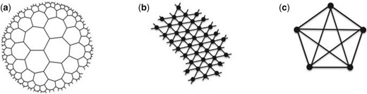
Examples of classic combinatorial structures, including (a) hyperbolic tiling (here triangle group |$\lbrace 2,3,7 \rbrace$|), (b) triangular lattice and (c) a |$d$|-regular graph with |$d=3$|.
![Set of exemplary real-world networks that we analyse throughout this article. This includes social (s, (1) Zachary’s karate club [21] and (2) social interactions of dolphins [23]), peer-to-peer (p, (3) email exchanges [24, 25]) and biological (b, (4) transcription, Escherichia coli (E. coli) [26]) networks.](https://oup.silverchair-cdn.com/oup/backfile/Content_public/Journal/comnet/6/5/10.1093_comnet_cnx049/1/m_cnx049f3.jpeg?Expires=1716427190&Signature=UgcqWiJ-zOsuEWEASVv4-ecFAaER68RbX92Ych9orhNbxSfg-yjzZiRdhbo9iPSO~ZeCNyMloa2EomeaF8EOKKH8Dt5ge62oI~lx0MPr1~XJ21jKBjbOzxa5zwGE8x02wbckot8GewTWxyLsciAH2ARajQJFc~75rbOZCz~FP8JakCU36HdsL0s6FR1zPxkiHq7UXvWu7BZaQfTDoWJnPSeELm8jdJkUXW62fRD6tHuxf5q6vJ8WlwBgPlrF-DTi5lIuYcu3Tc5FhJuirG-jjLUarE2i-nskfgHfPUNhRmvXENmWNpjuhGCaP~kOfR4Jcv3E52UWyBZdHCoNRwVjxQ__&Key-Pair-Id=APKAIE5G5CRDK6RD3PGA)
Set of exemplary real-world networks that we analyse throughout this article. This includes social (s, (1) Zachary’s karate club [21] and (2) social interactions of dolphins [23]), peer-to-peer (p, (3) email exchanges [24, 25]) and biological (b, (4) transcription, Escherichia coli (E. coli) [26]) networks.
2.1 2-faces
In the specific case |$p=2$|, we construct 2-faces|$f_d^2$| from simple closed paths between not interconnected |$n$|-tuple of nodes. We refer to the index |$d$| as the degree (or order) of the face. In the classic one-dimensional complex this refers to triangles between triples of edges, quadrangles between quadruples of nodes etc. To preserve the structural information of the one-dimensional complex, we introduce face weights |$\omega(f)$| according to an analogy from classic geometry: In [4], we consider ‘default’ edge weights |$\omega(e)$| from node weights in analogy to the length of a curve from the positions of its end points. For the two-dimensional case, we construct face weights from edge weights by the analogy of area computation, as follows:
- 1. Triangles|$\boldsymbol{(d=3)}$| We use Heron’s formula for the area of a triangle for given side lengths. In our setting, this gives for |$e_i \sim e_j$|, |$e_j \sim e_k$| and |$e_k \sim e_i$| (|$\sim$| denoting associations):(2.2)\begin{align} \omega (f_3^2) &=\sqrt{s (s- \omega(e_i)) \cdot (s-\omega(e_j)) \cdot (s- \omega(e_k))};\\ \end{align}(2.3)\begin{align} s &= \frac{\omega(e_i) + \omega(e_j) + \omega(e_k)}{2}. \end{align}
2. Polygons of higher degree |$\boldsymbol{(d>3)}$|
Triangulation: One could triangulate each |$n$|-dimensional polygon and use Heron’s formula to determine the area of the respective triangles (see above).
Imposing coordinates: Some real-world networks come naturally with ‘coordinates’, for example information about brain regions in brain networks or locations of resources in energy networks. In those cases, we can calculate the face weights from the edge weights using Gauß trapezoid formula, also known as Shoelace formula [22].
2.2 Use cases
We present statistics on the occurrence of higher degree faces (see Table 2). Later on, we will connect these statistics to theoretical results on the networks’ geometry. We consider the following types of use cases:
1. Combinatorial structures: Regular geometric structures that are constructed by simple combinatorial rules such as lattices and |$d$|-regular graphs;
2. Real-world networks: Complex networks inferred from empirical data.
Higher degree faces in combinatorial structures |$($||$^\ast:$| degree dependent|$)$|
| Hyperbolic tilings | Triangular lattice | |$K_5$| graph | |
|---|---|---|---|
| No. of nodes | N | N | 5 |
| No. of edges | |$\approx$|N | |$\approx$|N | 10 |
| No. of triangles | |$\approx {\rm \frac{1}{7}}$|N | |$\approx {\rm \frac{1}{3} }$|N | 10 |
| Average degree | 7 | 3 | 4 |
| Hyperbolic tilings | Triangular lattice | |$K_5$| graph | |
|---|---|---|---|
| No. of nodes | N | N | 5 |
| No. of edges | |$\approx$|N | |$\approx$|N | 10 |
| No. of triangles | |$\approx {\rm \frac{1}{7}}$|N | |$\approx {\rm \frac{1}{3} }$|N | 10 |
| Average degree | 7 | 3 | 4 |
Higher degree faces in selected real-world networks. We consider examples for social networks |$($|Zachary’s karate club [21], social interactions of dolphins [23]|$)$|, peer-to-peer networks |$($|email communications [24, 25]|$)$| and biological networks (transcription, Escherichia coli (E. coli) [26])
| Zarachy’s karate club | Dolphin’s interactions | Email communication | Transcription E. coli | |
|---|---|---|---|---|
| No. of nodes | 34 | 62 | 1133 | 79 |
| No. of edges | 78 | 318 | 12035 | 212 |
| No. of triangles | 45 | 95 | 982 | 130 |
| No. of quadrangles | 22 | 59 | 3434 | 17 |
| No. of pentagons | 5 | 145 | 5237 | 7 |
| No.of hexagons | 0 | 239 | 8560 | 4 |
| Average degree | 4.59 | 5.13 | 10.62 | 5.37 |
Ultimately, we are interested in the geometry of real-world networks. However, we develop our ideas starting from well-studied discrete structures (1) to draw from the rich body of work that has been done to characterize these objects.
2.2.1 Combinatorial structures
From the wide range of combinatorial structures, we choose hyperbolic tilings for their importance in geometric group theory and lattices and d-regular graphs as objects of major interest to graph theorists and probabilists. Among each class of geometric objects, we selected examples that are constructed from triangular basic structures allowing us to restrict our analysis to simplicial complexes (i.e. ‘filling in’ 3-faces).
2.2.2 Real-world networks
For category (2), we select real-world networks from different scientific disciplines (see Fig. 5). Notably, we observe two kinds of behaviour: networks, where we find more faces of higher degree than of lower and vice versa. We will later discuss a possible relation between this observation and the global geometry of these networks.
![Computation of auxiliary functions, illustrated on Zachary’s karate club [21].](https://oup.silverchair-cdn.com/oup/backfile/Content_public/Journal/comnet/6/5/10.1093_comnet_cnx049/1/m_cnx049f4.jpeg?Expires=1716427190&Signature=qH490VsIPoK6C4M4YCzFOWrpQmjAWeYS5CAhDOdHlRovLLm67cvYe4MjSfYDgHix7fyxPFihcMH-E12n6RhuBZtG4sTXrAYNcgFwi4ZdhLnjRCS8oFvtgKEZ7UZ1SB3jc8ZOwv6nuAy4-T-h-gwlbCrKrJmATdpLEHmEg3TneRTbtssAPw4Qa09FHtRlto1mTfC1eNRFNUdSNXRHoN8ZkfNkOuT1rdVlghOFMESqbn282EqDTeKXh1giZvIJNANP9d7ecxy1tKdOFshUHy6wBW7D~jrHvtVhQIhf27LgrZNJJsRRv6KzNaEUBNLXpIOOLR4gCRohgLz2IX38AKlBXA__&Key-Pair-Id=APKAIE5G5CRDK6RD3PGA)
2.3 |$n$|-faces
1. Unweighted (unit) edges
In the combinatorial case, that is if we assume unweighted edges, Eq. (2.4) simplifies [27] to(2.6)\begin{align} V(X) &=\frac{1}{n!} \det \left( \vec{e}_1, \vec{e}_2, ... , \vec{e}_n \right) \\ \end{align}(2.7)\begin{align} &= \frac{\sqrt{(n+1)}}{n! \cdot \sqrt{2^n}}. \end{align}From this, we get the following weighting scheme for |$n$|-faces (of degree 3):(2.8)\begin{align} \omega(f_{3} ^n)=\frac{\sqrt{n+1}}{n! \cdot \sqrt{2^n}}. \end{align}2.Perpendicular triangles
Alternatively, one could map the edge weights to Cartesian coordinates (see Fig. 4) yielding [27](2.9)\begin{align} X_i &= \omega (e_i) \vec{e}_i \\ \end{align}and therefore the weighting scheme(2.10)\begin{align} \Rightarrow V(X) &=\frac{1}{n!} \det \left( \begin{array}{ccc} \omega (e_1) \vec{e}_1 & \cdots & 0 \\ \vdots & \ddots & \vdots \\ 0 & \cdots & \omega (e_n) \vec{e}_n \end{array} \right) = \frac{1}{n!} \Pi_{i=1}^n \omega (e_i), \end{align}(2.11)\begin{align} \omega(f_{3}^n)=\frac{1}{n!} \Pi_{i=1}^n \omega (e_i). \end{align}
Construction of face weights.
For use cases of category (1) higher-dimensional equivalents can be obtained through simple extensions of the combinatorial construction rules to higher dimensions. In the case of less regular real-world networks (2), the possibility of filling in such structures needs to be evaluated computationally. In Table 3, we computationally detect higher dimensional faces (|$n$|-simplices) corresponding to higher order correlations in the previously considered real-world networks. The results are in accordance to the intuitive expectation that |$n$|-faces become increasingly rare with growing |$n$|.
| Zarachy’s karate club | Dolphin’s interactions | Email communication | Transcription E. coli | |
|---|---|---|---|---|
| No. of nodes | 34 | 62 | 1133 | 79 |
| No. of edges | 78 | 318 | 12035 | 212 |
| No. of 2-faces | 45 | 95 | 912 | 130 |
| No. of 3-faces | 11 | 27 | 745 | 38 |
| No. of 4-faces | 2 | 3 | 374 | 3 |
3. Forman–Ricci curvature in 2D
In [4], we introduce Forman–Ricci curvature and its associated flows, namely the Ricci flow and the Laplace–Bertrami flow, as characteristics for network graphs (i.e. one-dimensional, weighted cell complexes) with special emphasis on real-world networks. Now, we want to map this formalism to higher dimensions by defining Forman’s curvature for higher dimensional faces.
3.1 Forman-curvature
An interesting observation when constructing a two-dimensional complex from a one-dimensional graph can be made in the unweighted case: Adding a face of degree 3 increases the curvature of adjacent edges by 3, a face of degree 4 yields an increment of 2 etc. For faces of degree |$n$| we formulate the following lemma:
This lemma provides an easy computable formula for studying the Ricci curvature across large complex networks with consideration of higher degree faces. It is applicable for cases where the respective networks come unweighted, or can be mapped to an unweighted ones, by imposing a meaningful threshold with respect to the underlying data.
3.2 Bochner Laplacian
closely related to the Forman–Ricci curvature. As discussed in [5], this relation gives rise to a geometric flow, the Laplacian flow. For the one-dimensional case, the Laplacian flow has potential applications in the denoising of networks. Recall the general form of the Bochner Laplacian for |$p$|-dimensional cellular complexes [4, 6]:
4. Network-theoretic Gauß–Bonnet theorem and Euler characteristic
The failure to construct a Gauß–Bonnet theorem in the case of two-dimensional cell complexes results from the existence of ‘metrics’ of negative Forman–Ricci curvature (for every edge |$e$|) on any simplicial complex of dimension |$\geq 2$| (following from results of Gao, Gao–Yau and Lohkamp, see [6]). In more detail, a discrete analogue of the Gauß–Bonnet theorem does not hold for the derived Forman–Ricci curvature in dimension 2, since it implies that both the sphere and the torus can have negative curvature everywhere, which clearly contradicts the Gauß–Bonnet Theorem.
The absence of a fitting analogue of the Gauß–Bonnet theorem represents a serious disadvantage that diminishes the elegance of the other results. However, recently, an extension of Forman’s Ricci curvature was introduced by Bloch [7] that does provide a Gauß–Bonnet-type theorem for cellular complexes. We have recently introduced Forman’s Ricci curvature as a characteristic for networks viewed as classic graphs in one dimension and want to build on Bloch’s theoretical results for introducing a characterization of the shape of networks, using this formalism.
4.1 Bloch’s combinatorial Forman–Ricci curvature
As an edge-based characteristic per se, the Ricci curvature measures two-dimensional faces only to the extent of common boundaries of 2-faces. It follows that Eq. (4.2) is the relevant form of the Ricci curvature regardless of the dimensionality of the substructures (i.e. 2-faces or higher dimensional n-faces) of the complex.
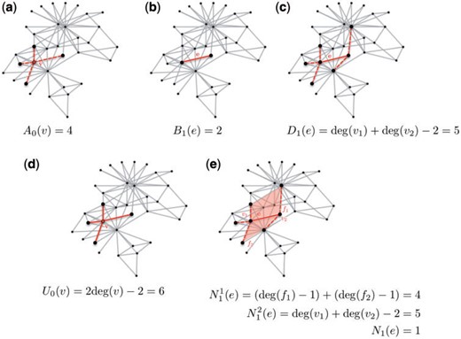
To formulate Bloch’s results, we first introduce some notation (in which we follow Bloch):
(Auxiliary functions) Let x be an |$i$|-dimensional face of a two-dimensional complex X.
1. |$A_i(x) = \# \{y \in F_{i+1}, x < y\}$|;
2. |$B_i(x) = \# \{z \in F_{i-1}, z < x\}$|;
3. |$U_i(x) = \sum_{y > x} B_{i+1}(y)$|;
4. |$D_i(x) = \sum_{z < x}A_{i-1}(z)$|;
5. |$N_i(x) = N_i^1(x) \Delta N_i^2(x)$|, with
|$ N_i^1(x) = \# \lbrace w \in F_i, \exists v \in F_{i+1} \; {\rm s.t.} \; x < v, w < v \rbrace $|,
|$ N_i^2(x) = \# \lbrace w \in F_i, \exists u \in F_{i-1} \; {\rm s.t.} \; u < x, u < w \rbrace $|.
Here |$\Delta$| denotes the symmetric difference and, by convention, summation over the empty set is considered to be zero.
(Curvature-functions) Let |$X$| be a two-dimensional cell complex. We define the curvature functions |$R_i:F_i \rightarrow \mathbb{R}$|, |$i = 1,2,3$| as
1. |$R_0 (v) = 1 + \frac{3}{2}A_0(v) - A_0^2(v);$|
2. |$R_1(e) = 1 + 6A_1(e) + \frac{3}{2}B_1(e) - U_1(e) - D_1(e);$|
3. |$R_2(f) = 1 + 6B_2(f) - B_2^2(f);$|
4.2 Network-theoretic Gauß–Bonnet theorem
We can now formulate Bloch’s—from our viewpoint—most important result:
In the context of the definitions above, we note:
1. The importance of Theorem 2 resides in the fact that it allows for defining prototype (or reference) networks for the Ricci flow in terms of a discrete curvature notion in strict analogy to the continuous case.
2. A sufficient condition for the equality (4.6) is that the intersection of any pair of 2-cells (faces) contains at most one 1-cell, that is an edge. Unfortunately, in the context of network graphs this condition fails in general: For instance, two edges adjacent to a vertex could be part of both a triangle and a quadrangle such that the triangle does not represent a subset of the quadrangle (i.e. they describe different types and orders of correlation).
3. Another potential issue are isolated edges in not-connected network graphs. By ‘pruning’ the leaves, that is by neglecting such edges we can apply the above discussed formalism. Generally, the theory applies only to connected graphs or large connected components—smaller degenerate structures need to be excluded from the analysis.
With this, we get a directly computable form of the Euler-characteristic:
Recently, after the first preprint of this version appeared on arxiv, Watanabe [30] proposed a different Gauß–Bonnet style theorem which also builds on Forman’s work. In contrast to our edge-based approach he introduces a scalar (Forman) curvature defined on the vertices of an unweighted graph.
4.3 A topological implication
One of the main strengths of Forman’s curvature resides in the fact that its sign provides information on the topology of the underlying complex. While not all of Forman’s results can be generalized to the case of Bloch’s extension, some topological implications can be transferred as we show in this section.
However, for this we have to pass to the mean curvature function |$R_1$| rather than using its edge-valued, basic definition. This is a consequence of the fact that |$R_1$| appears with a ‘-’ sign in the Gauß–Bonnet Theorem (4.7) above. Furthermore it explains, why we cannot expect to obtain the desired result in the most general case, but rather have to consider some (combinatorial) restrictions. These restrictions are [7], in increasing order of generality:
1. |$\overline{B}_1 \geq \frac{20}{9}$|, where |$\overline{B}_1 = \frac{1}{\# F_1}\sum_{e \in F_1}B_1(e)$|;
2. |$\overline{B}_1 = 2$| and |$\overline{A}_1 \geq 2$|, where |$\overline{A}_1 = \frac{1}{\# F_1}\sum_{e \in F_1}A_1(e)$|;
3. \((\overline{A}_1 + \overline{B}_1)^2 - 6\overline{A}_1 - \frac{3}{2}\overline{B}_1 - 1 \geq 0\).
The main result for the topological characterization of a complex in terms of the mean of |$R_1$|, that is |$\overline{R}_1 = \frac{1}{\# F_1 }\sum_{e \in F_1}R_1(e)$|, is the following:
(Bloch, [7], Theorem 2.7) Let |$X$| be a two-dimensional cell complex, satisfying any one of the conditions (1)–(3) above. If |$\overline{R}_1 >0$|, then |$\chi(X) > 0$|.
For the special case of two-dimensional, polyhedral complexes considered here, we obtain the following lemma:
Let X be a two-dimensional polyhedral complex with (1) |$\overline{A}_1 \geq 2$| and (2) |$\overline{R}_1 > 0$|. Then |$\chi(X)>0$|.
From this, we see that |$\overline{B}_1=2$| holds trivially, that is (2) simplifies to |$\overline{A}_1 \geq 2$|.
Since |$B_1 (e)=2 \; \forall e \in F_1$|, condition (1) is never fulfilled.
The conditions given by Lemma 4 link back to our earlier comment on the choice of polyhedral complexes as higher dimensional representations of networks. This choice imposes restrictions on both the connectivity and possibly occurring degenerated substructures. Lemma 4 only holds for complexes without isolated edges, that is not generally applicable to real-world networks. However, by ‘pruning the leaves’, that is by neglecting isolated nodes and edges, one can overcome this issue.
We compute |$\chi (X)$| for the previously considered real-world networks (Table 4) and combinatorial structures (Table 5). To limit computational expense, we only consider 2-faces of degree 3, that is triangles, that is, we restrict ourselves only to the special case of two-dimensional simplicial complexes. An interesting investigation extending the present study would be to include quadrangles, pentagons etc. and to analyse how the Euler characteristic changes for different types of networks. Note, however, that filling in large numbers of faces of dimension 2 or higher would lead to a simply connected complex, that is would represent a degenerate case of the formalism introduced in this article. Note also that, due to the large number of triangles, Euler characteristics can have large absolute values even for medium-sized networks. Taking into account that only the sign of |$\chi$| is truly relevant for our analysis (see discussion below), we compute and tabulate the mean Euler characteristic |$\overline{\chi} = \lfloor\overline{\chi}/\#T\rfloor$|, where |$\#T$| denotes the number of triangular faces.
Mean Euler characteristic |$\overline{\chi}$| for selected real-world networks. We consider examples for social networks (Zachary’s karate club [21], social interactions of dolphins [23]), peer-to-peer networks (email communications [24, 25]) and biological networks (transcription, E. coli [26]). |$^*$|: As discussed earlier, our formalism excludes degenerated substructures like isolated edges. The small, but positive |$\chi$| in this network is possibly an artifact introduced by the high number of such degenerated substructures resulting from the very small size of the network
| Zarachy’s karate club | Dolphin’s interactions | Email communication | Transcription E. coli | |
|---|---|---|---|---|
| No. of nodes | 34 | 62 | 1133 | 79 |
| No. of edges | 78 | 318 | 12035 | 212 |
| No. of 2-faces | 45 | 95 | 982 | 130 |
| |$\bar{\chi}(X)$| | 1|$^{\ast}$| | |${\rm 20 > 0}$| | |${\rm 15 > 0}$| | |${\rm -1< 0}$| |
Mean Euler characteristic |$\overline{\chi}$| for selected combinatorial structures. The sparse, combinatorial structures (tilings, lattice) have negative Euler characteristics, whereas the clique-like |$K_d$|-graph has a positive characteristic
| Hyperbolic tilings | Triangular lattice | |$d$|-regular graph (|$^\ast$| example: |$d=3$|) | |
|---|---|---|---|
| No. of nodes | N | N | 5 |
| No. of edges | |$\approx$|N | |$\approx$|N | 10 |
| No. of 2-faces | |$\approx {\rm \frac{1}{7}}$|N | |$\approx {\rm \frac{1}{3}}$|N | 10 |
| |$\bar{\chi}(X)$| | |$-381<0$| | |$-118<0$| | |$7>0$| |
An evaluation of the computed |$\overline{\chi} (X)$| and Tables 1 and 2 suggests that networks with a high number of high-degree faces have positive Euler characteristics. On the contrary, low numbers of high-degree faces might hint on negative Euler characteristics.
5. Ricci flow on two-dimensional complexes
We have extended the classical notion of the network to higher dimensions by adding |$n$|-dimensional faces and defined a Ricci curvature on those structures following previous, more general work of Forman [6]. Well appointed with these theoretical tools, we can now define associated curvature flows on the networks ‘surface’. For this, we build on previous work by E. Bloch and Chow and Luo (see [31]).
We assume here that curvature on the ‘surface’ will remain finite at all times, thus assuring the convergence to a unique connected reference space (prototype complex or prototype network). This assumption is motivated by results for the flow on smooth surfaces and by the work of Chow and Luo on the combinatorial flow. In the two-dimensional case we assume that we can achieve this finiteness by cutting faces without parents (isolated nodes and edges), that is those that are disconnected from the network’s ‘surface’. Note, that this assumption is not necessarily true for higher dimensional cases, that is one cannot hope to observe finite curvature in polyhedral 3-complexes, since for the classical analogue—the (smooth) flow on 3-manifolds—such ‘blow-ups’ of infinite curvature are known to occur [31]. Moreover, while there are algorithmic tools for combinatorial singularities arising in the surface flow, the three-dimensional case is far more complicated and no analogous method has been introduced so far [32].
5.1 Long-term flow and prototype networks
One would hope that the long term flow shares some essential properties with its classical counterpart, mainly the evolution—without the formation of singularities—to a prototype or reference space. In the classic case, both smooth surfaces under the classic Ricci flow [33], and piecewise-flat ones under the discrete flow [34], evolve to model surfaces of constant Gaussian curvature. In consequence, each compact surface (smooth or piecewise-flat) admits a background metric of constant curvature covered by the 2-sphere, the flat torus and the hyperbolic plane. Moreover, the limit surface (and hence its background metric) is determined by the topology of the surface, more precisely by its Euler characteristic.
Up to this point, there is no theoretical proof to support the role of |$\rm{\overline{Ric}_F}$| in concordance with that of |$\overline{K}$|. Moreover there is no established notion of Euler characteristics for an abstract, non-planar graph. Even if one could overcome this problem, one is still confronted with the failure of Forman’s curvature to satisfy a Gauß–Bonnet type theorem and hence the fact that there is no way to associate a limit surface (and a background geometry) to a given network. This shortcoming has largely motivated the present work.
Fortunately, the approach adopted here has two advantages: At first, it allows for a meaningful mean Ricci curvature and secondly, it satisfies a Gauß–Bonnet Theorem, thus enabling us to define prototype networks. We introduce prototype networks as minimal (in the sense of having the minimal number of 2-faces) two-dimensional polyhedral complexes with the Euler characteristics prescribed by the Gauß–Bonnet formula (4.7). In consequence, one can define a network to be spherical, Euclidean or hyperbolic, if its Euler characteristic is |$>, =$| or |$<$| 0, respectively:
(Prototype networks) Let X be a two-dimensional polyhedral complex with Euler characteristic |$\chi$| as given by the Gauß–Bonnet formula. Then we define |$\chi$| to be
1. Spherical, if |$\chi >0$|,
2. Euclidean, if |$\chi = 0$|,
3. Hyperbolic, if |$\chi <0$|.
While the minimality condition above is simple and intuitive, it seems that proving convergence of the flow using this definition is difficult. Therefore, in analogy with the classical (surface) case, we suggest to rather define prototype networks as having constant curvature in the limit, more precisely |$R_1 = {\rm const}$|. While the conjectured identity between the two approaches for defining prototype networks represents work in progress, let us only note that first experimental results seem to suggest that this is, indeed, the case.
By using Bloch’s results, we suggest a consistent notion of background geometry for networks that allows for the study of long term network evolution. This notion enables us to study such essential properties as (topological) complexity, dispersion of geodesics, recurrence, volume growth etc. that characterize a certain geometric type.
Surely, there are a number of limitations that still need to be overcome. Firstly, the formalism is restricted to the two-dimensional case, since with transition to dimensions 3 and higher the flow could develop the above discussed singularities. Secondly, for computational investigations one needs to remove isolated edges and nodes to avoid issues with degenerated substructures. For practical purposes this results in the restriction to limit the analysis to large connected components when imposing a higher dimensional connectivity condition since 1-connected graphs, etc. would render 2-complexes from having topological (cone) singularities.
A natural question arising in this context is how the above defined flow compares to similar geometric flows, starting with the simplest—the combinatorial flow. For the transition from the Forman–Ricci flow, defined on edges, to a flow on the two-dimensional complex we used the fact that the faces are just Euclidean (triangles)1, thus allowing for an extension from edges to faces by considering standard barycentric combinations.
5.2 Ricci flow and Laplacian flow
Here we consider the normalized long-term flow scaled with the mean Ricci curvature |$\overline{{\rm Ric_F}}$|, a global network property that is strongly related to the Euler-characteristic, as we have seen in the previous section.
Combining the Bochner–Weizenböck formula (Eq. 3.6) and the introduced Ricci-flow, we can define a Laplacian flow |$\Delta_F ^2$| for two-dimensional polyhedral complexes. We again only consider the combinatorial, thta is unweighted, case and set |${\rm Ric_F}=R_1$|:
5.3 Prototype networks
As previously discussed, we expect the Ricci flow to drive networks to structural limiting cases classified by the sign of their Euler characteristics. We termed these limiting cases prototype networks (Definition (5.1)). Figure 6 shows the evolution of two real-world examples [21, 23] with the discrete Ricci-flow acting on edge weights. We observe the evolution of the hyperbolic case and the spherical case as defined above. The degenerated Euclidean case with |$\chi=0$| is a rare limiting case that may occur by chance only in real-world examples, that is it is primarily of theoretical interest. At this point in time, a formal proof of convergence to these limit cases eludes us. However, first computational experiments indicate that indeed networks with |$\overline{{\rm Ric_F}} > 0$| tend to evolve to a more ‘round’, spherical shape, whereas those with |$\overline{{\rm Ric_F}} < 0$| evolve to more tree-like, hence hyperbolic structures.
For the combinatorial objects considered, Euler characteristics have negative signs (see Table 5). This is consistent with the geometric intution that structures like tilings and lattices are hyperbolic.
Our phenomenological exploration of the occurrence of higher degree faces in a small set of real-world networks suggested two distinct types of networks: Those for which we detected high numbers of 2-faces for higher degrees and others with a very low number of 2-faces of higher degrees. A comparison of this observation and the computed Euler characteristics suggests that the two types represent the two main classes of prototype networks that occur in real-world networks: spherical and hyperbolic. Spherical networks seem to be characterized by a high number of higher degree faces. They occur in densely connected substructures that possibly govern the evolution of the spherical type as illustrated in Fig. 6B. On the contrary, our hyperbolic examples show a rapidly decreasing number of detected faces when considering faces of higher degree. This lack of high degree faces seems to be linked to the rather sparse community structure that eventually evolves to a hyperbolic prototype network (illustrated in Fig. 6B).
![Prototype networks as limiting cases under the Ricci flow acting on edge weights. Edges with normalized weights below a threshold $0.05$ are considered to vanish. (a) Hyperbolic case. (network data: [21]). (b) Spherical case. (network data: [23]).](https://oup.silverchair-cdn.com/oup/backfile/Content_public/Journal/comnet/6/5/10.1093_comnet_cnx049/1/m_cnx049f6.jpeg?Expires=1716427190&Signature=vlJEjbNgCIb3KYbqIZjZX6HASaqDQ~66AO3pcbBikG5OCDk8lo4ROdblWjdsT6nlgOqM2b8UGFWzagx6n12OPeWmgdo0G2KsCAu8IRkgfFt9cfy27vuRMyjqf~aecwxXAPSo29-P6uXKR5uKLkInD2z2DPlIXw85ne3B2mObac21Vs-p~O6dTuZIPCV3nSsyx5Ii9eXpnFeSOLd~Nps4ykvH7QYHPerhYZSV3gbxx8twE5SzRMZGhfmPxmkNoivXP6ayMi2wzdGyylqXfvij8W9XCFfoWVYLcRLwb74ypIo4VLofzH5U~U1UocEnjYiJWdmZS2On6igIdGsBpeBY0g__&Key-Pair-Id=APKAIE5G5CRDK6RD3PGA)
6. Implications for real-world networks
After developing an abstract formalism for characterizing the shape of networks, we now want to put our results in the context of complex network analysis.
6.1 Higher degree faces and the ‘backbone’ effect
While ‘filling in’ higher degree faces marks, on an abstract level, the transition between classic graphs in one dimension and higher-dimensional polyhedral complexes, there exists a practical meaning of this transition for complex real-world networks. One important class of complex networks are correlation networks, where edges represent correlations between a system’s elements inferred from empirical data. The edge weights reflect the strength of the respective correlation. Such networks are widely used, especially in the life sciences. For instance, co-expression networks represent correlations in expression levels of genes and brain networks are typically inferred from correlations in the activity profiles of brain regions.
A 2-face of degree |$n$| then represents a sequence of |$n$| correlated elements (represented by nodes), for example for |$n=3$| we have elements |$A$|, |$B$| and |$C$| where |$A$| is correlated with |$B$|, |$B$| is correlated with |$C$| and |$C$| is correlated with |$A$|. By ‘filling in’ the respective triangle |$f_3^2=\lbrace A, B, C \rbrace$| we contract the three elements—curvature-wise—to one. An analogous observation can be made for higher degree 2-faces (see Lemma 1) and |$n$|-faces in general. Similar considerations apply to graph motives in other, not-correlation based complex networks.
The contraction itself is a meaningful reduction for most classes of complex networks and can be understood as representing the network at a higher level of abstraction: The elements (nodes) jointly represented by a |$n$|-face share commonalities and can be seen as a group or cluster with respect to this commonality. For example, in a social network, a |$n$|-simplex could represent a group of friends, co-workers, classmates or collaborators. Instead of representing every individual in the network, we compress them in groups; simplifying the computation of network properties, such as the Ricci curvature, by large scales. This transition to a higher level of abstraction is an intrinsic property of the higher degree Ricci curvature that we introduced in this article. In previous work [5], we discussed this very aspect in the one-dimensional case as the backbone-effect of the Ricci curvature, that is its ability to highlight essential topological and structural information.
6.2 Relation to dispersion
The observation of 2-faces in networks and the importance of this structural information has been made previously. We discuss a related approach from Social Network Science, namely the dispersion [35].
The edges that contribute to dispersion are parallels of |$e=e(u,v)$|, that is also contribute to the Ricci curvature of |$e$|. Therefore, the contraction that occurs curvature-wise when filling in faces also reduces dispersion. Closely related to the combinatorial (unweighted) Ricci curvature, the dispersion is an edge-based network property that—while also dependent on node degrees—strongly characterizes edge-based information.
To understand the close relation between the two measures, we go back to the analogy in classic Riemannian geometry. In a recent paper [5], we discussed and introduced Forman–Ricci curvature as a measure of geodesic dispersal (see Fig. 7A). The dispersion Eq. (6.1) gives a closely related network-theoretic counterpart to this idea. However, while closely related, we note that Eq. (6.1) is essentially a measure on triangles since it represents the number of triangles that feature a given edge |$e$| as a side. Therefore, in our classic analogy, this notions measures the volume (area) growth in the direction of the edge |$e$|, rather than the dispersion of geodesics. In consequence, dispersion is even more closely related to Ollivier’s discretization of Ricci curvature [36, 37] than to Forman’s. It is furthermore related to Stone’s Ricci curvature for |$PL$| manifolds [38].
![Dispersion in networks. (a) Dispersion of geodesics in the classic Riemannian case. (b) Dispersion between two associated nodes in a social network (Zarachy’s karate club, see [21]). The illustrated dispersion can be computed as ${\rm disp} (u,v)=5$ using Eq. (6.1).](https://oup.silverchair-cdn.com/oup/backfile/Content_public/Journal/comnet/6/5/10.1093_comnet_cnx049/1/m_cnx049f7.jpeg?Expires=1716427190&Signature=Zj8U6m6Swl1vXnnDKGF-KSoOLYGu-Ody3VEsstHDJnog95bplGdIgE5f2e4YsmjSavojFM4W1YFDcjqYvQB6RbIDk2UbPHGKvJqetP6JGngfeeEwS5EvBTlYKHLVM6KAYNv7zIrbhnwDDJpjEvu9EdgwMSY~g1HaB4u6EwoxQ0zcPf0SaakPrvlu7aBrrAn9JYUjg9TPrSgFOtSgl~HQUReHkltKj9xh47m2H6NlJCzc-Vliv3XDou3967cdCv~lpmyieJ6W8zvEh29ZsPvhAs9yWyCMxdkbfzyI4cqyiLPfUMsL6fKTB3wiusuXWd1oVW2TRRqQ2gy3qQSt0~693A__&Key-Pair-Id=APKAIE5G5CRDK6RD3PGA)
7. Discussion
In this article, we introduced a higher-dimensional representation of the classic one-dimensional graph model for networks that allows for analysis of ideal network shapes. By ‘filling in’ higher degree faces in sets of associated edges, we constructed two-dimensional polyhedral complexes that allow us to map the discrete Ricci-formalism we introduced in [4] to higher dimensions. In the following analysis, we mainly focused on filling in |$n$|-dimensional simplices.
Building on recent work by Bloch [7], we formulated a network-theoretic Gauß–Bonnet Theorem that allows for the definition of an Euler characteristic on networks. Furthermore, we introduced a first classification scheme for the shape of complex networks, so called prototype networks. Our results illustrate the backbone-effect of the Ricci-flow, that is its ability to provide an abstract of the topological and structural information of a network. It gives rise to a natural classification scheme for dynamically evolving networks based on topological properties. In contrast to previous approaches and model networks with an emphasis on node-based characteristics, the Ricci curvature and in consequence the Ricci-flow are edge-based. Defined by the information flow within the network, quantitatively described by the edge weights, both characteristics can be defined independently of node-based information overcoming the widely discussed node-degree bias present in most network-analytic tools. Furthermore, its focus on the information flow within a network makes the Ricci-formalism an ideal tool for the analysis of dynamics in networks.
While our study demonstrated promising results for the special case of two-dimensional simplicial complexes, the narrow range of cases we covered can only be considered preliminary. The emphasis of this article was to introduce theoretical tools and demonstrate their capabilities on a small set of use cases. Experiments with higher-dimensional cell complexes are needed for a full systematic study of the methods introduced in the present paper. Furthermore, the experiments undertaken so far were restricted to combinatorial networks. To understand more complex real-life networks, the computational experiments should be extended to weighted networks. Possible future directions include a broader study of two-dimensional polyhedral and CW cell complexes in an attempt to generalize the prototype networks introduced in this article.
A major direction for future research is the study of network evolution with the curvature-based methods introduced in this article. Future studies should be conducted in two directions:
1. Large-scale experiments on real-world networks with larger sample and network sizes to add statistical power to the preliminary results presented here.
2. The development of a theory accompanying and strengthening the proposed methods, namely by proving the (heuristic) convergence results and thus confirming that, indeed, the sign of |$\overline{{\rm Ric_F}}$|, determines the shape of the limiting prototype network.
A natural question in this context is, how—if at all—the presented formalism maps to 3-complexes. As discussed earlier, there are so far no general results or algorithmic tools to deal with the singularities that are known to occur in 3-complexes. It remains an open question, if there exists a network-theoretic counterpart to G. Perelman’s surgery method for the Riemannian case that might solve the singularity issue for the discrete case. Furthermore, one would seek to devise a more unified Ricci flow that incorporates the edge weights (as analogues of distances in the Riemannian setting), as well as node weights that represent discretizations of (curvature) measures concentrated at certain points (on a manifold).
Further directions for future study include:
1. The actual extraction of algebraic-topological information from higher dimensional networks (i.e. unoriented hyper-networks/simplicial complexes), which includes the computation not only of |$H_1(N)$|, in terms of the positivity of the Forman–Ricci curvature, but also, in similar terms, of |$H_p(N)$| (see [6], Corollaries 2.9 and 4.3), as well as the estimates on |${\rm dim}H_p(N)$| (cf. [6], Theorems 4.4, 4.6 and 4.7). Moreover, via a fitting discretization of Myers’ Theorem this could provide information on the finiteness of |$\pi_1(N)$| (thus providing in fact even stronger results for the understanding of the topological complexity of the (hyper-)network than Persistent Homology (see also [19]).
2. The extraction of the geometric ‘backbone’ that captures structurally important edges acting as bridges between major network communities.
3. Since the Forman–Ricci curvature and its higher dimensional counterparts come coupled with a corresponding Laplacian [5], one could study (hyper-)networks by means of these graded Laplacians. This would allow for an understanding of their structure at the level of all degrees of connection. Specific tools and methods would include eigenvalues (and eigenfunctions) that already proved efficient in the classification of networks [39].
The present article introduced novel prototype networks in a first attempt to classify networks by counterparts of common tools from Differential Geometry: The Gauß–Bonnet theorem and Euler characteristics. We showed that one can seemingly predict the limiting case of a network’s evolution based solely on its Ricci curvature. Linking back to our initial question, we can see the shape of a network—by only evaluating its Ricci curvature.
Acknowledgements
E.S. thanks Moses Boudourides for bringing the notion of dispersion to his attention. Furthermore, he would like to thank the Max Planck Institute for Mathematics in the Sciences, Leipzig, for its support and warm hospitality. M.W. was supported by a scholarship of the Konrad Adenauer Foundation.
Supplementary data
Implementations used for conducting computational experiments are publicly available on Github: MelWe/networkcharacterization.
Footnotes
1 In fact, this can be done mutatis mutandis for spherical triangles as well.
