


Abstract
BACKGROUND: Quantification of changes in semen may give insight into the testosterone (T)-induced disruption of spermatogenesis in man. METHODS: A model analogous to flushing of sperm from the genital tract after vasectomy was used to quantify the time course of semen changes in subjects participating in male contraceptive trials using 800 mg T-implant (n = 25) or 200 mg weekly intramuscular injection (IM-T; n = 33). A modified exponential decay model allowed for delayed onset and incomplete disruption to spermatogenesis. Semen variables measured weekly during a 91-day period after initial treatment were fitted to the model. RESULTS AND CONCLUSIONS: Sperm concentration, total count, motility and morphometry exhibited similar average decay rates (5 day half-life). The mean delay to onset of decline in concentration was 15 (IM-T) and 18 (T-implant) days. The significantly longer (P < 0.005) delays deduced for the commencement of fall in normal morphology (41 days), normal morphometry (40 days) and sperm viability (43 and 55 days), and the change of morphometry to smaller more compact sperm heads are consistent with sperm being progressively cleared from the genital tract rather than continued shedding of immature or abnormal sperm by the seminiferous epithelium. A significant negative relationship was found between lag time and baseline sperm concentration, consistent with longer sperm-epididymal transit times associated with lower daily production rates.
Introduction
Male hormonal contraceptive (MHC) regimens aim to induce uniform and reversible azoospermia using safe and acceptable drug formulations. Administration of a pharmacological dose of testosterone (T) by intramuscular injection of testosterone enanthate (TE) or subdermal implant of depot T reduces pituitary LH and FSH secretion and thereby sperm production. For a majority of men, sperm concentration is suppressed to azoospermic or severely oligospermic levels (WHO, 1990; 1996; Handelsman et al., 1992). The addition of a progestin enhances spermatogenic suppression and allows the use of more physiological T regimens (Handelsman et al., 1996). However, despite such improvements, not all men suppress to azoospermia. Turner et al. found ∼5% of 55 men treated with a depot progestin and androgen combination failed to suppress sperm concentrations below 1 × 10⁶/ml. As with other regimens, they also found a wide range in the rate at which individual men suppressed, as measured by the percentage decrease of sperm output at 1 month from commencement of treatment compared with baseline (Turner et al., 2003). A better understanding of the source of these differences may assist in the development of a regimen that will uniformly induce azoospermia.
To develop better targeted and more effective MHC regimens it may also help to establish whether men who fail to suppress to azoospermia represent those for whom spermatogenesis is only partially shut down, or whether these men exhibit the hypospermatogenesis pattern of a general reduction in all germ cell elements with normal maturation. There have been conflicting reports of reduced sperm function in T-induced oligospermic samples (Wu and Aitken, 1989; Liu et al., 1995; Wang et al., 1997), but pregnancies have been reported in male contraceptive trials in men with severe oligospermia during the suppression and efficacy (<5 × 10⁶ sperm/ml) phases (WHO, 1996). The site of the disruption to spermatogenesis and the fertilizing capacity of sperm in T-induced oligospermic samples may be reflected in specific changes in sperm morphology during suppression. Automated image analysis offers reproducible quantification of many morphological characteristics of sperm, providing a particularly sensitive tool for identification of treatment or exposure-induced changes within an individual, or changes within an individual sample resulting from a procedure or physiological process. The sensitivity of our sperm morphometry system has been demonstrated previously by the identification of morphometric selectivity in the human sperm–zona pellucida binding process (Garrett and Baker, 1995; Garrett et al., 1997). This system was used in the present study to examine the detail of morphometric changes during T-induced suppression of spermatogenesis.
In terms of the mechanism of MHC action, both semen analysis and the stereological assessment of testicular tissue can be used to understand the regression of spermatogenesis. Testicular biopsies indentify T-induced impairment of spermatogonial development as an observed decline in type B followed by type Ap spermatogonial number (McLachlan et al., 2002). However, there must also be a major disruption at sperm release in both acute and chronic MHC-induced gonadotropin withdrawal, since control numbers of elongated spermatids are seen in the epithelium after 6 weeks of T treatment when the number of sperm in the ejaculate is reduced to severe oligospermic levels (Zhengwei et al., 1998b; McLachlan et al., 2002). Indeed, the general rapid loss of sperm in the ejaculate does not reflect the lesion in spermatogonial development but is consistent with a major disruption to the later processes of spermiogenesis or spermiation (Meriggiola et al., 1996; Turner et al., 2003).
Because spermatogenesis occurs at a constant rate and the timing of the cell division is known, the site and type of gonadotrophin-induced disruption to spermatogenesis may be inferred from the time course of changes in semen analysis, including the appearance of immature cells in the ejaculate. The present work seeks to quantify the observed time course of these T-induced changes, particularly with respect to sperm concentration and morphology, and thus facilitate analysis and interpretation of the different patterns of suppression response. To this end, we have chosen the simplest mathematical model consistent with known physiological information to fit the measured decline in sperm concentration. The rate of disappearance of sperm from the ejaculate following vasectomy has been measured and indicates a classical exponential decrease, with each successive ejaculation expelling ∼70% of sperm remaining distal to the point of vasectomy (Figure 1) (Freund and Davis, 1969). Similarly, sperm concentration in successive ejaculations over a 24-h period has been found to decrease approximately exponentially, with ∼50% clearance per ejaculation (Bedford, 1994). By analogy, if evidence points to an acute T-induced shutdown of spermatogenesis at a specific stage in the cycle, a model to quantify the experimental time course for sperm concentration would describe an exponential decrease from the baseline level, commencing at a time-dependent on treatment response time, epididymal transit time and the site of disruption to spermatogenesis. Also, given that it is known from stereological evaluation that all tubules within an individual do not necessarily respond homogeneously to T treatment (Zhengwei et al., 1998b), the exponential decay would asymptote toward a value directly related to the overall degree of suppression or completeness of disruption to sperm production. The time course would only asymptote to zero in the case of suppression to azoospermia. The model parameters extracted from the fit to the data therefore include the rate or half-life of the decline from baseline, the lag time describing the delay to onset of decline, and the asymptotic value of the decline. As there is no evidence to suggest otherwise, for our model and interpretation of results we assume that exogenous T does not influence the rate of spermatogenesis or the mechanism of sperm clearance.
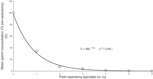
Rate of disappearance of sperm from the ejaculate following vasectomy. The raw data were taken from a study of 13 men by Freund and Davis (1969) and for each subject the sperm concentrations were calculated relative to the pre-vasectomy sample at time 0 and the resulting mean was fitted to an exponential decay curve as indicated.
Concerning the expected pattern of change for other semen variables such as motility and morphology, two patterns can be postulated. If the T-induced decline in sperm production is due to a rapid shutdown of spermatogenesis in a proportion of seminiferous tubules, sperm in the post-treatment ejaculate would represent a combination of sperm from reduced but normal continuous production and normal sperm suffering from progressive degradation or ageing during the flushing process. The resultant time course would be strongly dependent on the proportion of sperm in each category. Alternatively, if the induced sperm suppression mimics the situation of oligospermia as seen commonly in subfertile men where semen variables are universally poor, then one would expect a simultaneous decline in morphology and motility with concentration.
This study involved examining changes in semen variables in the Melbourne participants in two MHC trials: a multicentre intramuscular T (IM-T) trial conducted by the WHO (1996) and a more recent T-implant trial (McLachlan et al., 2000). A relatively low T dose (800 mg) was chosen for the T-implant trial to provide incomplete spermatogenic suppression in some men, in order to test for improvement in contraceptive efficacy by co-treatment with a 5α-reductase inhibitor (finasteride), commenced at the second implant at 3 months. The expected slower and minimal response to the low-dose T-implant, together with more frequent sampling in this trial, provided the opportunity to examine morphometric changes during suppression of spermatogenesis that had not been possible in the previous IM-T trial.
Materials and methods
Subjects and study design
Healthy volunteers aged 21–45 years old were recruited from the general community for a clinical trial of the contraceptive efficacy of 3 monthly T-implants to induce severe oligo- or azoospermia, the details of which have been published previously (McLachlan et al., 2000). Two baseline semen samples were collected prior to treatment and volunteers with both pretreatment sample concentrations <20 × 106/ml were excluded from the trial. Twenty-six of the men recruited at the Royal Women’s Hospital subsequently received a subdermal abdominal implant of 4× 200 mg pellets of fused crystalline T (Organon, Sydney, Australia). Weekly semen samples after 2 days abstinence were requested during the suppression phase until contraceptive efficacy was established and semen was then monitored at monthly intervals. For the purposes of this study of the suppression phase, only data from semen samples collected less than 91 days after administration of the initial T dose were analysed. This avoided complications arising from either a second implant or recovery from the original implant. With one exception, the 26 recruited subjects provided sufficient semen samples during the initial 3 months of the suppression period for the time course analysis (mean of 10 samples/subject). During the first 91days a total of six pellets were spontaneously expelled in four subjects, but expulsion was no earlier than 3 weeks post-implant (mean 54 days; range 21–87 days). There were no other side-effects of the treatment during the study period.
Semen data for 33 Melbourne participants in a multicentre male contraceptive study undertaken by the WHO (1996) were re-analysed for comparison with the T-implant data. In the WHO study, two pretreatment samples were required to meet the same concentration criterion of >20 × 106/ml, but subjects were treated with weekly intramuscular injections of 200 mg TE and samples were requested every 2 weeks after 2–5 days abstinence. A mean of seven samples/subject were analysed for the period up to 91 days from the first T injection.
Results from the 85 patients selected for sperm concentration between of 3–10 × 106/ml from a previous study of subfertile couples (Garrett et al., 2003) were used in the comparison of sperm morphometry between pathological and induced oligospermia.
Semen analysis
Semen specimens were collected by masturbation. Semen volume, sperm concentration, total and progressive motility, and viability were measured by standard techniques (WHO, 1992). Total count for an ejaculate is the product of semen volume and sperm concentration.
For morphology assessment, the semen samples were washed with 0.9% NaCl to remove the viscous seminal plasma and re-suspended to a standard concentration of ∼80 × 106/ml. Air-dried smears were fixed with ethanol and stained using the Shorr method (Jeulin et al., 1986) and cover-slipped for protection. The morphology assessment of a sample was performed manually by an experienced observer using a modified strict application of the WHO criteria (WHO, 1992), with particular emphasis on the normality of the acrosome region (Liu and Baker, 1994). Where the sperm concentration exceeded 3 × 10⁶/ml, the morphometry of each sample was also assessed using our fully automated image analysis system (Garrett and Baker, 1995). In all cases 200 sperm were assessed per sample. The morphology was expressed as a percent normal (%N) and the morphometry as a set of means and standard deviations for each of the 32 morphometric parameters, in addition to a percent conformity (%C) of sperm with parameters within 2.5 SD of a reference set of ‘normal’ means (Garrett and Baker, 1995).
Data analysis
Morphometric differences before and after T-implant. In general, automated morphometric analysis could not be carried out on samples with sperm concentrations <3 × 10⁶/ml. For the T-implant subjects, changes in each sperm morphometry parameter were evaluated by paired t-test on the difference between the mean baseline value and the mean of the last two analysable samples collected post-implant. Owing to the large number of morphometric parameters (n = 32), statistical significance for difference was set using the Bonferroni correction to P < 0.05/32 = 0.0016 in this analysis. An increase in the sperm misidentification rate for this fully automated system is anticipated for samples with low sperm concentrations, since they are usually associated with an increase in the ratio of debris to sperm in the smear. Thus, to check that the morphometric changes observed following suppression of sperm production were not an assessment artefact, these data were also analysed after application of an additional more stringent ‘debris filter’ in the image analysis which eliminated all imaged objects with area <4.5 µm2.
Morphometry was not performed for the IM-T trial.
Time course for semen variables. The hypothetical time course is parameterized by the equations and illustrated by the graph depicted in Figure 2. The parameter c represents the baseline value of the semen variable Y, whilst b is the parameter defining the minimum value to which this variable asymptotes following treatment at time t = 0. Thus, a non-zero value of b for sperm concentration or total count indicates incomplete suppression of sperm production. The parameter t0 defines the time lag from treatment to the onset of the exponential decrease observed in semen variable Y. The parameter a describes the rate of decrease of Y with time, where the half-life for the decay is related by τ½ = ln(2)/a. A zero value of a indicates no change in Y with time.
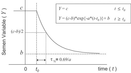
A hypothetical time course for semen variable Y in ejaculates from a subject treated with testosterone at time t = 0, represented by a constant value c, prior to the lag time t0, followed by an exponential decay at rate a, to the suppressed level, b.
Using unweighted least squares fitting between this model and the measured data for each subject, a set of the time course parameters a, b, c and t0 can be established for each of the semen variables. The values of the deduced parameters are expected to differ between subjects and between semen variables. Particularly in the case of sperm concentration and total count, the time course analysis is expected to be influenced by the variability in the frequency of ejaculation between sample collections. For the ideal application of the model, semen analysis measurements would correspond to sequential ejaculates. Extra ejaculations between the samples analysed would have greatest influence early in the suppression phase, biasing the deduced results to a higher decay rate and, to a lesser extent, shorter lag time than if sequential ejaculations were measured. The effect on parameters b and c would be minimal. The influence of extra ejaculations is expected to be higher in the IM-T study because samples were only analysed every 2 weeks.
For each subject in both the IM-T and T-implant trials, a set of time course parameters was extracted for sperm concentration, total count, total motility and viability. In addition, for the T-implant trial the time course of the morphometry and morphology assessments of %C and %N were also available for analysis. Azoospermic samples obtained within the 91 day study period were included in the fit to the model for sperm concentration and total count but not for other semen variables. Differences between the time course parameters a, t0 and the non-dimensional ratio b/c for each of the semen variables were evaluated using paired t-tests. Relationships between the time course parameters were also examined by linear regression analysis.
Ethics
The study was approved by The Royal Women’s Hospital Research and Ethics Committees and the subjects consented to the research on their gametes.
Results
Morphometric differences before and after T-implant
Of the 32 parameters used to define sperm head morphometry, 10 showed significant (P < 0.0016) changes between pre- and post-treatment T-implant samples where there was suppression of sperm concentration (Table I; Figure 3). These changes in morphometry after treatment were of small magnitude: a general decrease in head size (8% mean decrease in head area A) with a greater loss in length (L, 6.5% decrease) than width (W, 2.3% decrease). Two parameters related to the anterior staining of the head (Bill and e90) were also significantly different, indicating a change toward a more uniform optical density of the sperm head in samples during suppression of sperm concentration. There was no significant increase in cytoplasm in the neck or droplets in post treatment semen samples. In fact, the neck area parameter (nA) decreased by 11%. These results remained essentially unchanged when the data were re-analysed after application of the additional ‘debris filter’, which eliminated all imaged objects with an area <4.5 µm2 (Table I).
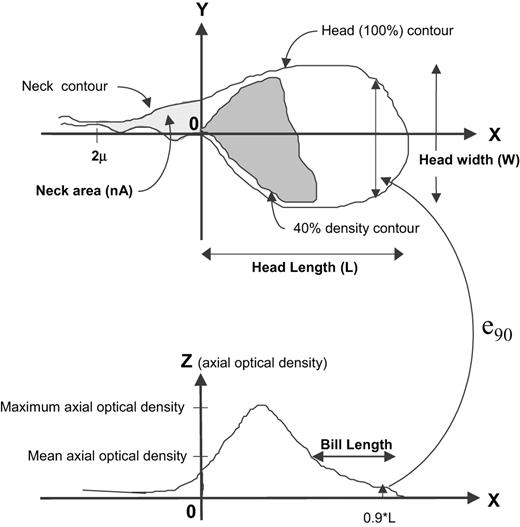
Schematic diagram of the imaged sperm head illustrating some of the morphometric parameters that changed significantly after T-implant.
For the same morphometric parameters, differences between the means for 85 infertility patients with 3–10 × 106/ml sperm concentration and the means for the baseline samples for the 24 T-implant subjects are included for comparison in Table I. For all the parameters listed in Table I except nA, the patient oligospermic samples show a greater difference from baseline compared with the induced oligospermic samples. This is particularly evident for the optical density derived parameters that are related to acrosome region of the head (Bill, e90). The optical density anterior length parameter (ZaL) had the greatest percentage difference for the oligospermia patients compared with baseline values, but did not show significant change during T-induced suppression.
Time course for semen variables
Representative time course data and fitted curves for sperm concentration and the morphometric %C assessment for four subjects after 800 mg T-implant are shown in Figure 4. One subject in the T-implant trial exhibited no suppression of sperm concentration in the model fitting procedure (a = 0) and was not included in subsequent analysis of the model parameters. The means and standard errors for the parameters of the fitted time course for each of the semen variables measured in the T-implant trial (n = 24) are listed in Table II and summarized graphically in Figure 5. The mean results for the fits to the time course data for the 33 subjects in the IM-T trial are included in Table II. Since the absolute values of the parameters b and c cannot be directly compared between semen variables, the ratio b/c (%), which is a measure of the degree of suppression, is also included in Table II.
Mean baseline values and T-induced differences for the 10 morphometric parameters showing significant differencesa
| SHAMAS parameterb | Units | Code | Mean baseline | Mean difference | Mean difference (>4.5 µm2 filter) | Difference of means (patients – baseline) |
|---|---|---|---|---|---|---|
| Head length | µm | L | 4.55 | −0.30 | −0.25 | −0.36 |
| Head width | µm | W | 3.02 | −0.07 | −0.05 | −0.13 |
| Head area | µm2 | A | 10.53 | −0.87 | −0.73 | −1.3 |
| Anterior head length | µm | aL | 2.17 | −0.12 | −0.10 | −0.21 |
| Head perimeter | µm | P | 13.01 | −0.65 | −0.54 | −0.70 |
| Neck area | µm2 | nA | 1.68 | −0.18 | −0.19 | −0.11 |
| 40% density shape factor | SF40 | 1.13 | 0.03 | 0.03 | 0.06 | |
| Optical density centroid length | % | ZcL | 57.33 | −0.64 | −0.60 | −1.7 |
| Bill length | % | Bill | 35.26 | −1.8 | −1.5 | −6.3 |
| 90%L transverse ellipticity | e90 | 0.317 | −0.04 | −0.04c | −0.11 |
Shown are the mean baseline values and T-induced differences for the 10 morphometric parameters showing significant (P < 0.0016) differences between the means of the last two analysable post-treatment samples and the two baseline samples, for the T-implant subjects where sperm concentration was suppressed (b/c <100%; n = 24). Also, mean differences with the more stringent ‘debris filter’ and differences for oligospermic patients (n = 85) relative to the means for the baseline samples of the T-implant subjects.
See Figure 3 and Garrett and Baker (1995).
P = 0.0021.
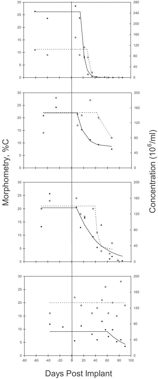
Time course data and fitted curves for sperm concentration and normal morphometry (%C) for four T-implant trial subjects. The graphs were chosen to show differences in rates and levels of suppression, as well as differences in magnitude of the variation about the fitted curves.
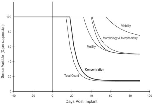
Average suppression curves corresponding to the mean values of the time course parameters from the fit to the semen data for the 24 T-implant subjects of Table II. The semen variables have been normalized to a pre-suppression mean value of 100%.
The mean sum of least squares for the fit to the model for the total of 57 subjects was compared with the mean sum for a simpler vasectomy clearance model with no lag time (t0 = 0) or residual spermatogenesis (b = 0). The physiological model of this study provided the better fit but because of the wide variability of the data the improvement in goodness of fit did not quite reach significance (P = 0.07).
The t0 values for normal morphology (%N), normal morphometry (%C) and sperm viability were significantly different (P < 0.005) from those for sperm concentration and total count. Both %N and %C assessments of the T-implant trial showed similar lag times that were significantly longer than the corresponding times for sperm concentration and total count (Table II). In both T-implant and IM-T trials, sperm viability had the longest mean delay to onset of decline and sperm motility exhibited an intermediate delay.
Mean (SEM) [LQ-median-UQ] results for the time course parameters for semen variables for subjects where sperm concentration was suppressed (b/c <100%) in the IM-T (n = 33) and T-implant (n = 24) contraceptive trials
| Semen variable | c | b | b/c (%) | a (days–1) | t0 (days) | ||||||||||
|---|---|---|---|---|---|---|---|---|---|---|---|---|---|---|---|
| IM-T | T-implant | IM-T | T-implant | IM-T | T-implant | IM-T | T-implant | IM-T | T-implant | ||||||
| Concentration (106/ml) | 100 (8) [66-102-124] | 109 (12) [61-99-141] | 2 (1) [0-0-21] | 16 (5) [0-0-26] | 3 (1)a [0-0-0] | 16 (5)a [0-0-21] | 0.15 (0.01) [0.10-0.14-0.22] | 0.15 (0.02) [0.06-0.15-0.25] | 15 (2) [0-12-24] | 18 (3) [5-15-24] | |||||
| Total count (106) | 319 (30) [197-325-378] | 344 (44) [185-327-439] | 9 (2) [0-0-0] | 47 (14) [0-19-66] | 3 (1)a [0-0-0] | 15 (4)a [0-8-24] | 0.15 (0.01) [0.08-0.14-0.21] | 0.15 (0.02) [0.05-0.19-0.25] | 9 (3) [0-9-12] | 14 (3) [0-15-20] | |||||
| Total motility (%) | 71 (1) [65-73-76] | 64 (1) [59-66-68] | 36 (4) [24-42-51] | 32 (5) [5-37-50] | 52 (5) [35-58-77] | 49 (7)b [8-60-77] | 0.11 (0.02) [0.02-0.08-0.20] | 0.10 (0.02) [0.01-0.05-0.25] | 22 (5) [0-17-29] | 32 (5)b [18-24-44] | |||||
| Viability (%) | 85 (1) [82-86-87] | 83 (1) [80-83-87] | 59 (5) [49-65-78] | 58 (6) [38-67-80] | 70 (6) [56-77-100] | 70 (7)b [46-80-100] | 0.03 (0.01) [0.00-0.01-0.03] | 0.05 (0.02)b [0.01-0.05-0.25] | 43 (7) [11-26-90] | 55 (7)b [21-60-90] | |||||
| %N | 20 (2) [12-21-25] | 10 (2) [3-9-15] | 51 (7)b [22-45-86] | 0.10 (0.02) [0.01-0.09-0.20] | 41 (6)b [18-30-71] | ||||||||||
| %C | 20 (1) [16-19-25] | 10 (2) [4-9-18] | 50 (7)b [15-44-77] | 0.14 (0.02) [0.05-0.15-0.25] | 40 (6)b [14-41-57] | ||||||||||
Significantly different (P < 0.01) between IM-T and T-implant data.
Significantly different (P < 0.005) from associated concentration and total count time course parameter (paired t-test, pooled IM-T and T-implant data).
LQ = lower quartile; UQ = upper quartile.
In both trials, the mean degree of suppression was significantly greater for sperm concentration and total count compared with the other measured semen variables. Suppression of sperm concentration and total count was also significantly greater for IM-T subjects (b/c = 3%) compared with T-implant subjects (b/c = 15%). Only viability measurements showed a significantly different rate of decay from other semen variables, indicating a comparatively slow decline with time. Good agreement was observed between all fitted time course parameters for the manual and computer-assessed morphology data.
For sperm concentration there was no significant correlation between the baseline time course parameter (c), and either the rate (a) or degree (b/c) of suppression after treatment. Nor was there any relationship between the rate and degree of suppression. A significant negative linear relationship was found between the lag time parameter t0 and the baseline c, in both T-implant and IM-T trials (Figure 6). Lag time was not related to either rate or degree of suppression. Similar results were obtained for the total sperm count parameters. For all measured semen variables, the mean lag time to onset of decline was shorter for the subjects treated with intramuscular injection of 200 mg TE than for those treated with 800 mg T implant (Table II), but the differences were not significant by t-test.
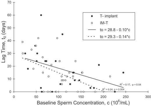
The relationship between the lag time for sperm concentration, t0, and the pre-suppression concentration, c, for both T-implant and IM-T trial data.
Discussion
In this study a mathematical modelling approach has been used to describe the patterns of suppression of semen parameters during the onset of MHC, with IM-T and T-implant, in order to identify the physiological changes in sperm and deduce the likely site of impact of acute gonadotropin withdrawal on spermatogenesis. We conclude that the less marked and longer lag times for the decline in motility and morphology than in sperm concentration are consistent with ageing changes in sperm being cleared from the genital tract, rather than a continued shedding of immature or abnormal sperm by the gonadotrophin-deprived seminiferous epithelium. Also, the mean/median delay to onset of decline in sperm concentration was 15/12 days (IM-T) and 18/15 days (T-implant), consistent with epididymal transit following a rapid disruption to spermatogenesis at spermiation. In both trials, a significant negative relationship was found between lag time and baseline concentration.
The minimal changes measured for specific sperm morphometry parameters after T-implant support the contention that spermatogenisis is disrupted at spermiation, although the increase in the ratio of seminal debris to sperm in sequential samples as the sperm number declines introduces the possibility that the measured changes are an artefact of the progressive increase in the computer misidentification rate of sperm. However, the observed morphometry changes remained after an additional size threshold was applied as a more stringent ‘debris filter’. In addition, the substantial agreement between the changes in the computer assessment %C and the manual morphology assessment %N indicates that the decrease in %C is unlikely to be simply related to an increase in misidentification rate of sperm using the automated system.
In the rat, T-induced gonadotrophin suppression disrupts maturation of round to elongated spermatids and is accompanied by the sloughing of round spermatids into the genital tract (O’Donnell et al., 1996). This does not occur in the human, since round spermatid number in the semen has been reported to decrease in parallel with sperm concentration during T-induced suppression of spermatogenesis (Zhengwei et al., 1998a). While our automated morphometric analysis system cannot detect immature sperm specifically, there was no evidence of an increase in neck area or width that would be expected if sperm with cytoplasmic droplets were more prevalent in semen after T treatment. In fact, the observed decrease in head size parameters, particularly those related to the region of the low optical density at the anterior of the head, are consistent with chromatin condensation associated with an increasingly mature sperm population in samples collected during the suppression phase (Bedford et al., 1973).
Although it is known from stereological evaluation that a major site of disruption to spermatogenesis with gonadotrophin suppression in man is at the spermatogonial stage, the relatively rapid decline of sperm in the ejaculate indicates that later stages must also be affected. The lag time to onset of this decline results from the time required for absorption of the exogenous androgen, suppression of gonadotrophins, the site of disruption to spermatogenesis and the transit time of sperm through the genital tract. The relative time courses for these processes are indicated schematically in Figure 7. Time course data for several semen variables were fitted to a mathematical model representing a delayed but rapid disruption to spermatogenesis.
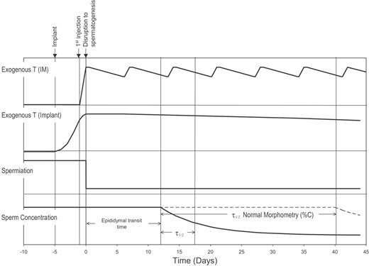
Schematic diagram of T levels in blood after administration by IM or implant and the relative lag times associated with the influence of the exogenous T on spermiation, sperm concentration and percent normal morphometry in semen calculated from the mean results of the time course analysis and epididymal transit time.
Because of the variability in the data a variety of models could fit the data in a statistical sense, but we chose to fit a model based on the physiology. The assumption of an exponential decrease is supported by both post-vasectomy and rapid multiple ejaculation data for sperm concentration and total count, which have evacuation of sperm reserves at a rate defined by a deduced ‘half-life’ of between 0.6 and 0.9 ejaculations (Freund and Davis, 1969; Bedford, 1994). The use of time rather than ejaculation number in our model assumes a regular and universal frequency of ejaculation, which is not practical with human subjects. Variations in the subjects’ ejaculation frequency would contribute to fluctuations about the general trends (Figure 4) and would not be expected to have a major effect on the mean results for the parameters of the model, but could bias results towards shorter half-life values. However, the mean rate of decrease of sperm concentration or total sperm count (a = 0.15) converts to a 4.6-day half-life and is of the order of one abstinence period (2–5 days), consistent with the approximately one ejaculation half-life indicated by the vasectomy and rapid multiple ejaculation data. This similarity in rates of decline also suggests that the T-induced disruption at spermiation is a relatively sharp discontinuity, represented schematically in Figure 7 as a step function. Individuals were found to exhibit varying degrees of suppression of sperm concentration with lag times ranging from ∼0 to 60 days after T-implant and from 0 to 42 days after IM-T. While this heterogeneity may reflect variation in sperm-epididymal transit times or disruption at different sites in the spermatogenic process, it could merely result from differences in ejaculation timing, variable proportions of residual sperm expelled per emission or errors of measurement influencing the model fitting procedure. In some cases the scatter of the data is large relative to the decline in concentration and the least squares fitting is relatively flat across all values of lag time, as in the extreme case of the 60-day lag time (bottom graph Figure 4). Selective removal of such data would tighten the deduced estimates of time course parameters but would lose objectivity.
Striking between subject differences in the degree of spermatogenic inhibition have been observed in stereological studies (Zhengwei et al., 1998b; McLachlan et al., 2002). Our model takes into account this variability in the degree of disruption by allowing the change in semen variables to asymptote to a value other than zero. The lack of relationship between the lag time (t0) or rate of decline (a) with the degree of suppression (b/c) for sperm concentration is consistent with a common disruption site in a varying proportion of tubules in each subject.
The 3–5 day shorter lag time to onset of decline in sperm concentration and total count following IM-T injection compared with T-implant is not statistically significant, but a longer period to induce effective gonadotrophin suppression is not unexpected for the implant study. It is possible that a higher frequency of extra ejaculations within the 2-week collection interval in the IM-T study may account for the difference. Lower frequency of ejaculation immediately after T‐implant owing to abdominal soreness would similarly influence the results but is considered unlikely. IM-T is expected to affect gonadotrophin secretion within a day, since plasma T levels are very high by this time and 24-h infusion of T affects secretion of LH and FSH within this period (Anderson and Wu, 1996; Wang et al., 1998). Thus, ∼12 days of the lag time for suppression of sperm concentration and total count can be attributed to a combination of the epididymal transit time and the time taken for cells to proceed from the final site of major disruption in the spermatogenic process to spermiation.
Indirect estimates of sperm transit time in the human epididymis based on stereological studies of testes after castration vary from 2–6 to 19–23 days (Rowley et al., 1970; Amann and Howards, 1980; Johnson and Varner, 1988). Rowley et al. used radiolabelling and X-ray irradiation as markers to measure transit times. They found that on average, most sperm took ∼12 days to transit the genital tract, with a 1–21 day variation within the individual (Rowley et al., 1970). Our deduced lag time to onset of suppression therefore appears to be of the order of the sperm-epididymal transit time. We have also found an inverse relationship between lag time and baseline sperm concentration (Figure 5). Johnson and Varner (1988) reported longer sperm-epididymal transit times in men with low daily sperm production rates compared with those in men with high daily sperm production rates.
The fact that the mean lag time is found to be equivalent to the sperm-epididymal transit time suggests a significant disruption to sperm production at spermiation, the final stage of spermatogenesis. Testicular biopsies reveal that T-induced gonadotrophin suppression produces a major disruption in spermatogenesis at the transition from type A to type B spermatogonia (Zhengwei et al., 1998b). However, if this were the sole lesion, the observed time lag should include an additional 42-day delay associated with the continued development of germ cells previously produced from spermatogonia and already present in the seminiferous epithelium (Clermont, 1963). If the major disruption occurred, as in the rat, during maturation of round to elongated spermatids (human stage III–IV) without affecting later stages, a lag time of ∼16 days longer than the transit time would be expected (O’Donnell et al., 1994).
To develop better targeted and more efficient MHC regimes it is of a general interest to establish whether men who fail to suppress to azoospermia represent those for whom spermatogenesis is only partially disrupted, or whether these men exhibit the hypospermatogenesis pattern of general impairment of sperm function. The morphometry changes during T-induced suppression are significant, but not large compared with the corresponding differences observed between the means for infertile patients with oligospermia and the baseline values of the study subjects. In particular, differences in the optical density derived parameters for the patient samples were two to four times greater than those for the T suppressed samples, with the greatest difference for the patients observed in the ZaL parameter, which was not found significantly different for the trial subjects. These optical density parameters (Bill, e90, ZaL) are related to the acrosome region of the head and have previously been identified as important factors for natural fertility (Garrett et al., 2003).
There are conflicting reports about sperm quality during T‐induced oligospermia. Early work using the zona-free hamster oocyte penetration assay suggested that induced suppression of spermatogenesis caused defective sperm maturation and in-vitro fertilizing capacity (Wu and Aitken, 1989). Interpretation of the results of the work is confounded by false-negative results at low sperm concentrations, which the authors claimed to circumvent by increasing oocyte number and mathematically correcting to a constant motile sperm concentration. A more recent study did not confirm these results (Wang et al., 1997). In addition, the ability of sperm to bind and penetrate the zona pellucida of human oocytes was not found to be severely impaired in T-induced oligospermic samples (Liu et al., 1995). Pregnancies at sperm concentrations of <5 × 10⁶/ml during treatment of men with gonadotrophin deficiency and during male contraceptive trials also suggests significant fertilizing capacity of sperm in men with oligospermia associated with low gonadotrophin levels (Burger and Baker, 1984; WHO, 1996). The specific morphometric changes observed in sperm during the suppression phase in this study were consistent with induced oligospermia representing partial spermiation failure with normal sperm aging during the flushing process.
In summary, modelling the time course of change in semen variables, including sperm morphometry, during the T-induced suppression of spermatogenesis has provided general support for a rapid disruption to spermatogenesis at spermiation in all or a majority of seminiferous tubules. The effect of the disruption is observed in the semen as an exponential decline in sperm concentration and total count, commencing after a treatment lag time commensurate with T delivery and sperm epididymal transit. The less marked and significantly longer lag times for the decline in the other semen variables are consistent with this concept that sperm in post-treatment semen are from unaffected tubules and clearance of residual sperm in the genital tract.
The authors gratefully acknowledge the assistance of research nurses Debbi Rushford and Jillian McDonald, and laboratory assistance of Ming Li Liu BSc of the Royal Women’s Hospital, Melbourne, Australia. We also thank Howard Wraight of Organon, Sydney, Australia for donation of testosterone pellets for the male contraceptive trial. This study was supported by the Sperm Research Fund, Melbourne IVF, Melbourne, Australia and the World Health Organization, Human Reproduction Program, Project ID 97128 and 89903.
References
WHO (
WHO (
WHO (
Author notes
1Department of Obstetrics and Gynaecology, University of Melbourne and Reproductive Services, Royal Women’s Hospital, Melbourne, Victoria 3053 and 2Prince Henry’s Institute of Medical Research, Monash Medical Centre, Clayton, Victoria 3168, Australia
