


Abstract
We report on the near-infrared matches, drawn from three surveys, to the 1640 unique X-ray sources detected by Chandra in the Galactic Bulge Survey (GBS). This survey targets faint X-ray sources in the bulge, with a particular focus on accreting compact objects. We present all viable counterpart candidates and associate a false alarm probability (FAP) to each near-infrared match in order to identify the most likely counterparts. The FAP takes into account a statistical study involving a chance alignment test, as well as considering the positional accuracy of the individual X-ray sources. We find that although the star density in the bulge is very high, ∼90 per cent of our sources have an FAP <10 per cent, indicating that for most X-ray sources, viable near-infrared counterparts candidates can be identified. In addition to the FAP, we provide positional and photometric information for candidate counterparts to ∼95 per cent of the GBS X-ray sources. This information in combination with optical photometry, spectroscopy and variability constraints will be crucial to characterize and classify secure counterparts.
1 INTRODUCTION
Astrophysical X-ray sources range from extragalactic objects such as galaxy clusters and active galactic nuclei (AGN) to Galactic sources such as supernova remnants, coronally active stars, pulsars, accreting systems containing compact objects and even some Solar system bodies. The X-ray continuum observed in all these sources comes from different processes such as bremsstrahlung radiation, synchrotron radiation, blackbody radiation, inverse Compton scattering and atomic recombination.
All-sky X-ray surveys were created with NASA's first Earth-orbiting X-ray-only mission, Uhuru (Giacconi et al. 1971) and have been updated since then with many various X-ray missions (e.g. HEAO: Nugent et al. 1983; RXTE: Levine et al. 1996; ROSAT: Voges et al. 1999; Anderson et al. 2003, 2007). Also, many all-sky X-ray monitors have been used to detect, identify and follow-up Galactic X-ray transient sources (e.g. RXTE: Orosz et al. 1998; Remillard 1999; Ratti et al. 2012; Swift: Zhang et al. 2007; Muñoz-Darias et al. 2013; MAXI: Kuulkers et al. 2013). ESA's XMM satellite also plays an important role in surveying the X-ray sky (Watson et al. 2003, 2009). The brightest X-ray point sources in Galactic environments tend to be accreting compact objects, making X-ray surveys a straightforward method to detect them.
In our Milky Way, multiwavelength studies of X-ray source populations have mainly been carried out in the Galactic Centre (Muno et al. 2004, 2009; Mauerhan et al. 2009; DeWitt et al. 2010) and the Galactic plane (Grindlay et al. 2005; Servillat et al. 2012; van den Berg et al. 2012; Nebot Gómez-Morán et al. 2013) by exploiting the Chandra X-ray Observatory's excellent spatial resolution. The Centre suffers from extremely high extinction and crowding, making multiwavelength follow-up of the X-ray sources very difficult. In most studies, it was found that a simple astrometric and photometric matching was not enough to find the true counterparts to the X-ray sources and additional photometric and spectroscopic data were required to confidently find the real matches. Moreover, the main focus so far has been on systems bright in the optical and/or near-infrared (NIR), making most confirmed sources giants, high-mass X-ray binaries, which contain early-type mass donors and cataclysmic variables (CVs). The extinction drops off rapidly away from the Galactic Centre making the follow-up study of X-ray sources considerably less challenging in the rest of the Galactic plane and bulge. The Galactic bulge, also highly populated with X-ray sources due to the fact that it contains about 14 per cent of the mass of the Milky Way (McMillan 2011), suffers from three times less extinction in E(B − V) than the Centre, making it a more practical region to study the Galactic X-ray population. Besides their detection, the identification of X-ray sources is crucial in these surveys. With this in mind, the Galactic Bulge Survey was designed (GBS; Jonker et al. 2011).
In this paper, we search for, characterize and discuss the NIR counterpart candidates to the GBS X-ray sources. The NIR data were taken from the VISTA Variables in the Via Lactea Survey (VVV; Minniti et al. 2010), the Galactic Plane Survey (GPS; Lucas et al. 2008) from UKIRT Deep Sky Survey (UKIDSS) and the Two Micron All Sky Survey (2MASS; Skrutskie et al. 2006). In Section 2, we begin with a description of the different surveys, then in Section 3 move on to compare all three NIR surveys in order to show how each one can be used for different purposes. Section 4 is then dedicated to constraining the extinction towards the GBS fields. Then, we discuss the false alarm rate in finding the real NIR counterpart to the X-ray sources in Sections 5 and 6.
2 SURVEYS DESCRIPTION
2.1 Galactic Bulge Survey (GBS)
The GBS combines sensitivity for faint X-ray sources, the astrometric accuracy of the Chandra X-ray Observatory, with a complementary photometric optical r′, i′ and Hα survey (Jonker et al. 2011). The GBS has several goals which will mainly be accomplished with the discovery of accreting compact objects. Detecting X-ray accreting objects is necessary in order to understand binary formation and evolution (Jonker et al. 2011). X-ray binary systems are numerous in their types such as low-mass X-ray binaries (LMXBs) which contain a neutron star or a black hole accreting matter from a low-mass companion (M < 2 M⊙), ultracompact X-ray binaries (UCXBs) which are LMXBs with orbital periods shorter than one hour. CVs, which consist of a white dwarf accreting matter from a late-type dwarf, are not usually classified as X-ray binaries even though they are binary systems and do emit X-rays. Binary systems are crucial for the determination of masses of compact objects, offering strong constraints on stellar evolution. In terms of our understanding of binary evolution, the common envelope phase is not yet well understood, therefore finding compact binary sources which have undergone one or two common-envelope phases will help us further understand that crucial evolutionary phase. The more binary systems we find in a well-controlled sample, the better our constraints of binary formation and evolution will be. This can be done by comparing robust samples against predictions from population synthesis calculations. Such samples can be constructed by counting the number of sources of a given class in a well-controlled area. This results in a necessary tool in the study of X-ray sources, the need to classify sources. Although the X-rays allow us to pinpoint possible accreting objects, more detailed follow-up through the detection of coincident counterparts at other wavelengths is necessary. Thus, multiwavelength studies of the GBS X-ray sources, as well as spectroscopic follow-up form a key component of our strategy (radio: Maccarone et al. 2012; optical: Hynes et al. 2012; optical variability: Britt et al. 2013, spectroscopic: Britt et al. 2013; Ratti et al. 2013; Torres et al. 2013).
The area of the sky covered in this survey is two rectangles of l × b = 6° × 1°, centred at b = ±1| $_{.}^{\circ}$|5 (see Fig. 1). These two strips were chosen in order to avoid the Galactic Centre region (|b| < 1°), which suffers from extremely high extinction and source confusion, while the source density is still high. The GBS is a shallow X-ray survey, of 2 ks exposures, in order to maximize the fraction of sources that are LMXBs, while also ensuring that a large fraction of the detected sources are suitable for spectroscopic follow-up. Theoretical calculations from Jonker et al. (2011) predict the detection of ∼1600 X-ray sources in the survey region, out of which ∼700 are expected to be coronally active late-type stars (single and binaries) or binary systems such as RS Canum Venaticorum (RS CVn) or W Ursae Majoris (W UMa) systems, ∼600 are CVs and ∼300 are LMXBs.
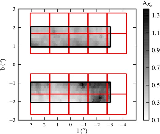
The GBS coverage. The black boxes indicate the GBS region. In red, we show the VVV pointings which were used for the search of the NIR counterparts of the X-ray sources. The grey colour scale indicates the strength of the extinction value in the Ks band (|$A_{K_{\rm s}}$|) towards the GBS fields (see Section 4 for more details).
The GBS completed the total 12 deg2 area of the survey in both the X-ray and optical bands. Two separate X-ray energy bands (0.3–2.5 keV and 2.5–8 keV) were used to distinguish between soft and hard X-ray sources. A total of 1658 X-ray sources, with more than 3 X-ray counts, were found in the total area covered by the Chandra X-ray Observatory (see Fig. 1). Jonker et al. (2011) published the initial list of X-ray sources detected between 2009 and 2010, containing 1234 sources. In 2011–2012, Chandra observed the remaining observations of the survey, adding another 424 X-ray sources to the list (Jonker et al. 2014). We use the source list and same naming convention as in Jonker et al. (2011). It is important to note that out of the initial list of published objects in Jonker et al. (2011), Hynes et al. (2012) found 18 duplicates, meaning that our catalogue actually contains 1640 unique X-ray sources. The main reason why duplicate sources were found in the catalogue was due to the fact that they were faint and off-axis, leading to a large point spread function (PSF) and poor centroiding. In our study, we will use the original catalogue of 1658 sources and comment on the duplicates in our final table containing the NIR data of their matches.
2.2 The NIR surveys
We exploit NIR data of the bulge region in order to find the counterparts of the GBS X-ray sources. Here, we present three NIR surveys which nominally cover the GBS fields: 2MASS, UKIDSS GPS and VVV. All three surveys have a different depth and coverage, each offering specific advantages in the search for the NIR counterparts of the GBS sources.
2.2.1 The Two Micron All Sky Survey (2MASS)
2MASS is an NIR survey, using the J, H and Ks filters, which began in 1997 June and was completed in 2001 February, covering 99.998 per cent of the celestial sphere (Skrutskie et al. 2006). It produced a Point Source Catalog containing 471 million sources and an Extended Source Catalogue of 1.7 million sources. In order to map out the entire sky, 2MASS required telescope facilities in both hemispheres. Two identical 1.3 m equatorial telescopes were constructed for the survey's observations. The northern telescope is located at the Whipple Observatory at Mount Hopkins in Arizona (USA) and the southern telescope was constructed at the Cerro Tololo Inter-American Observatory at Cerro Tololo in Chile. An automated software pipeline, the 2MASS Production Pipeline System (2mapps), reduced each night's raw data and produced astrometrically and photometrically calibrated images and tables. The entire 2MASS data set was processed twice. The average pixel scale is 2 arcsec per pixel. The astrometric accuracy of the 2MASS catalogue is better than 0.1 arcsec for sources with Ks < 14 (Skrutskie et al. 2006).
This survey is reliable for sources with magnitudes up to 15.8, 15.1 and 14.3 in J, H and Ks, respectively (Skrutskie et al. 2006), in regions which do not suffer from high densities of sources. In the bulge, the depth is around 1.5 mag shallower (see Table 1). For this reason, we use 2MASS magnitudes solely in the case of bright sources (Ks < 11.5) where the other deeper NIR surveys saturate.
2.2.2 UKIDSS Galactic Plane Survey (GPS)
UKIDSS is the UKIRT (United Kingdom Infrared Telescope) Deep Sky Survey, which began in 2005 May. It consists of five different surveys, each covering different areas of the sky, with the use of five NIR broad-band filters (ZYJHK) as well as a narrow-band one (H2), and with a total area of 7500 deg2 (Lawrence et al. 2007). These surveys all use the Wide Field Camera (WFCAM), mounted on UKIRT, a 3.8 m infrared reflecting telescope located on Mauna Kea in Hawaii. The projected pixel size is 0.4 arcsec and the total field of view is 0.207 deg2 per exposure. The data are reduced and calibrated at the Cambridge Astronomical Survey Unit (CASU), using a dedicated software pipeline. They are then transferred to the WFCAM Science Archive in Edinburgh.1 The nominal positional accuracy of UKIDSS is ∼0.1 arcsec but this deteriorates to 0.3 arcsec near the bulge (Lucas et al. 2008).
The GPS maps the Galactic plane in JHK to a latitude of ±5°. The Galactic longitude limits are 15° < l < 107° and 142° < l < 230°. An additional narrow region, with |b| < 2° and −2° < l < 15°, will also be mapped in GPS. Thus, the UKIDSS GPS overlaps fully with the GBS fields. However, coverage is not as complete as originally intended. We use data from DR8 of GPS, where the coverage in the K band is about 65 per cent complete, whereas the J and H bands are still at about 35 per cent complete. The total survey area of GPS is 1800 deg2, in JHK to a depth K ∼ 18 mag (Lucas et al. 2008). This 5σ limiting magnitude is given for non-crowded regions. In the Galactic Centre and bulge, the depth of the survey is shallower (see Table 1). UKIDSS GPS data saturates when the magnitudes in JHK reach J < 12.75, H < 12.25 and K < 11.5 (Lucas et al. 2008).
2.2.3 VISTA Variables in the Via Lactea (VVV)
VISTA (Visible and Infrared Survey Telescope for Astronomy) is a 4 m class wide-field telescope, located at the Cerro Paranal Observatory in Chile. Its main purpose is to conduct large-scale surveys of the southern sky, in the NIR wavelength range. The camera mounted on VISTA is VISTA InfraRed CAMera, which is a wide-field NIR camera with an average pixel scale of 0.34 arcsec per pixel. The total effective field of view of the camera is 1.1 × 1.5 deg2. The broad-band filters used are Z, Y, J, H and Ks, with bandpasses ranging from 0.8 to 2.5 μm (Minniti et al. 2010; Saito et al. 2012).
VVV is a public NIR variability European Southern Observatory (ESO) survey. Its main goal is to construct the first precise 3D map of the Galactic bulge by using variable stars such as RR Lyrae stars and Cepheids (Minniti et al. 2010; Saito et al. 2012), which are accurate primary distance indicators. The survey plan is to cover 520 deg2 of the Galactic bulge and an adjacent section of the mid-plane. The Milky Way bulge area which will be covered expands from l < |10|° and −10° < b < +5°, thus covering the GBS area. In our study, we use data from all five filters provided in VVV. The depth and exposure times in each band are given in Table 1. The pipeline used to process the VVV data is based at CASU2 and delivers reduced and calibrated images, as well as the aperture photometry for the VVV fields.
Exposure times and 5σ limiting magnitudes in all three NIR surveys used in this paper. The GPS integration times are longer than those applied in VVV, allowing for deeper observations of the bulge than VVV. The magnitude limits given here are for fields that are moderately crowded similar to the GBS areas.
| Survey | Filters | Exposure time (s) | Depth (mag) |
|---|---|---|---|
| 2MASS | J | 7.8 | 14.3 |
| H | 7.8 | 13.6 | |
| Ks | 7.8 | 12.8 | |
| J | 80 | 18.5 | |
| UKIDSS GPS | H | 80 | 17.5 |
| K | 40 | 16.5 | |
| Z | 40 | 18 | |
| Y | 40 | 18 | |
| VVV | J | 48 | 17 |
| H | 16 | 16.5 | |
| Ks | 16 | 16 |
We merged all the Z, Y, J, H and Ks catalogues for each GBS source in order to work on the magnitudes and colours of any possible matches located near the X-ray positions. In order to test the quality of the photometry of the VVV data, we plot the magnitude errors against magnitudes of the nearest VVV match to the GBS sources, in all five filters (Fig. 2). This gives us an indication of the limiting magnitudes of the VVV pointings we are using. Due to the dense fields of the bulge, the actual depth is sensitive to seeing and thus covers a range around the nominal depth quoted in Table 1. Note that VVV data saturates at Ks ≲ 11.5 mag.
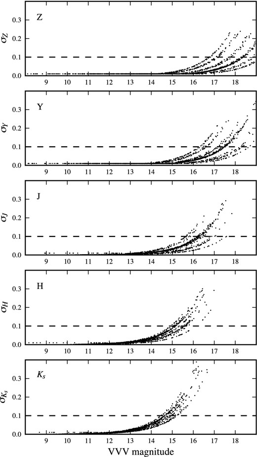
We plot the magnitude against its uncertainty for different VVV fields. The typical 5σ limits of sources located in the Galactic bulge are given in Table 1. It is clear that the different VVV fields do not have the same depth due to seeing variations from observations taken on different nights. This explains the large spread seen in the limiting magnitude values.
3 NIR COVERAGE OF THE BULGE
In this section, we compare the NIR surveys under consideration in order to show in which context each survey can be best employed. 2MASS will be useful in the case of saturated sources in VVV and UKIDSS GPS. We also show that UKIDSS GPS goes deeper than VVV, yet it does not cover the entire GBS area yet, making VVV the one with the most uniform coverage, in terms of both survey area and depth.
3.1 Coverage
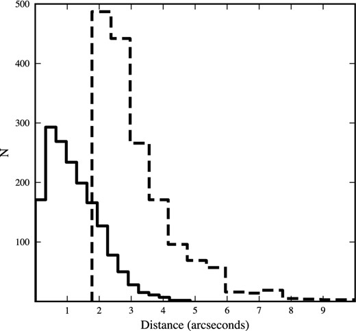
Distribution of distances to the closest VVV matches within 5 arcsec of the X-ray position (solid) and the 95 per cent confidence positional X-ray uncertainty of each GBS source (dashed). It is clear that the positional uncertainty can become very large in some cases making it impossible to choose the correct NIR match from positional coincidence alone.
Percentage of total number of valid detections found within a 5 arcsec (upper section) radius and 2.8 arcsec (lower section) of the X-ray positions, in 2MASS, UKIDSS GPS (DR8) and VVV.
| Survey | Z | Y | J | H | K | JHK |
|---|---|---|---|---|---|---|
| 2MASS | – | – | 74.7 | 74.7 | 74.7 | 74.7 |
| UKIDSS GPS | – | – | 34.9 | 35.2 | 63.8 | 31.5 |
| VVV | 98.1 | 98.7 | 99.3 | 99.5 | 99.5 | 99.2 |
| 2MASS | – | – | 48.7 | 48.7 | 48.7 | 48.7 |
| UKIDSS GPS | – | – | 34.3 | 34.6 | 61.5 | 31.1 |
| VVV | 85.3 | 86.9 | 91.3 | 92.2 | 91.7 | 88.4 |
We now turn to compare the NIR matches found in 2MASS and GPS with respect to the VVV matches, since the latter is the most complete survey out of the three in terms of coverage.
3.2 VVV versus 2MASS
When comparing the magnitudes of the closest matches within 5 arcsec of the X-ray positions in 2MASS and VVV, we find a small magnitude range where both surveys are in agreement. The J- and H-bands magnitudes agree between ∼12 and ∼14th mag, the Ks band ones between ∼11.5 and ∼13th mag. However, 2MASS is more reliable at the bright end, for magnitudes <12 in J and H and <11.5 in Ks, whereas VVV is more reliable in the case of fainter magnitudes. Therefore, in the case of bright sources, we use 2MASS when their NIR magnitudes are available (see Table 2 for the number of sources with 2MASS data).
3.3 VVV versus UKIDSS GPS
Similarly to the work done with 2MASS, we compare the VVV matches of the GBS sources with those found in GPS. The magnitudes seem to agree in the ranges of ∼12 to ∼15 mag in all three bands (see Fig. 4). Bright sources in both surveys do not agree due to saturation problems. On the fainter end, VVV becomes less reliable and therefore starts to deviate from UKIDSS. The scattered points seen between both surveys can be explained by several reasons: many sources in the intermediate-magnitude range are probably blended objects or possibly variable sources. Variable sources will be followed up in detail in a future paper. The different pipelines, filter sets and photometric systems used can also contribute towards the offsets between both surveys (clearest in the Ks band), indicated with the horizontal lines in Fig. 4.5 However, GPS is not yet complete and only contains matches to ∼35 per cent of the X-ray sources in J, H and K, whereas VVV covers over ∼99 per cent of the GBS fields.
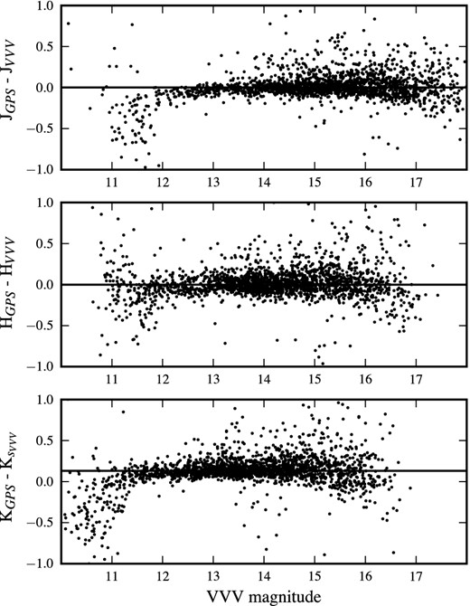
Difference between the VVV and UKIDSS GPS magnitudes against magnitudes in J, H and Ks. The solid horizontal lines correspond to the median of the difference in magnitudes between both surveys.
As seen in Table 1, GPS goes deeper than VVV. In order to confirm this statement as well as the nominal depth given in Table 1 for VVV, we show in Fig. 5 the distribution of the fraction of number of sources detected in GPS and VVV, as a function of the Ks-band magnitude. For each GBS source that has both UKIDSS GPS and VVV detections, we look for the number of GPS detections (NGPS) and the number of VVV detections (NVVV) within a given the Ks-band magnitude bin. We then calculate ΔN = NGPS − NVVV, for each source, and divide by NGPS. Finally, we take the mean value of all |$\frac{\Delta _N}{N_{\rm GPS}}$| in a given magnitude bin (shown in Fig. 5). When the fraction is negative, this indicates that there are more VVV detections in the considered the Ks-band magnitude bin. When ΔN ∼ 0, both surveys are in agreement and when the fraction reaches 1, GPS dominates over VVV. We see that both surveys are on par until Ks ∼ 16, where the VVV source catalogues become significantly incomplete, at least in the Galactic bulge regions considered here. We further conclude that blending appears not to be the limiting factor over the whole GBS area given that the median seeing of the GPS is 1 arcsec (Lucas et al. 2008) whereas that of the VVV is 0.8 arcsec.
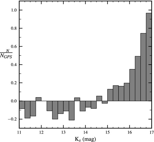
Distribution of the fraction of detected sources UKIDSS GPS (NGPS) and VVV (NVVV) as a function of Ks magnitude. ΔN corresponds to (NGPS − NVVV). From the increase towards 1 in the ratio towards fainter magnitudes, we conclude that the UKIDSS GPS limiting magnitude is larger than that of VVV (see text for more details). We further conclude that crowding is not a limiting factor over the whole GBS area given that the median seeing of the GPS is 1 arcsec (Lucas et al. 2008) whereas that of the VVV is 0.8 arcsec.
Because we wish to have a consistent photometric system which covers a broad range of wavelengths and almost the entire solid angle of the GBS, we primarily use VVV for the search of the NIR counterparts to the X-ray sources in GBS, and use 2MASS in the case of bright matches. Our comparison shows that this gives us a secure picture of all viable counterparts down to K ∼ 16. We also report on any UKIDSS GPS detections with Ks > 16 (see Section 5.6). Note that the comparison between VVV and other NIR surveys was only possible in the JHKs bands since those were the only filters in common with 2MASS and UKIDSS GPS.
4 EXTINCTION
The typical E(B − V) value towards the GBS fields is ∼1.8, clearly indicating that the survey region suffers from high extinction. We note that the measured E(B − V) by Gonzalez et al. (2011) is integrated to typical distance of RC stars. Therefore, for each GBS source, the returned E(B − V) value can be lower or higher, depending on its distance.
5 RESULTS
For 99.6 per cent of the GBS sources, we now have NIR data from VVV in Z, Y, J, H and Ks. When data were available, we created a small catalogue with all the NIR objects found within 10 arcsec of the X-ray position. Most sources returned over 10 neighbours, which clearly reflects on the multiple possible matches found for each X-ray source (see Fig. 6, right). We also have an approximate reddening value for most GBS sources (see Fig. 1), as well as their X-ray properties from Jonker et al. (2011). For each Chandra source, we created a postage stamp with five VVV finder charts (10 × 10 arcsec2), in each filter, as well as three colour–colour diagrams: (Z − Y, Y − J), (Y − J, J − H) and (J − H, H − Ks) (see Fig. 7). We included ZYJHKs isochrones6 in the VISTA photometric system, in order to know where the un-reddened main-sequence stars lie. These colour–colour diagrams and postage stamps were used by us to identify possible targets for spectroscopic follow-up in order to classify likely counterpart candidates. More details on the spectroscopic component of the GBS is given in Torres et al. (2013). While these individual data sheets offer detailed insights into the specific environments around our X-ray sources, we now turn to a more robust statistical study of the counterpart candidates detected in the NIR in order to identify those that may be considered genuine NIR matches.
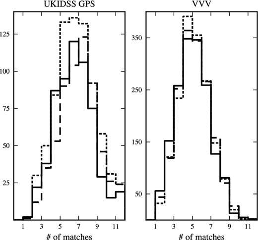
Distribution of the number of matches found in UKIDSS GPS (left-hand panel) and VVV (right-hand panel) within 5 arcsec of the X-ray position out of the total number of 1658 GBS X-ray sources. The solid line corresponds to the J band, the dashed line to the H band and the dotted line to the K band. Note that the reason why the total number of sources (y-axis) in GPS is smaller than in VVV is due to the larger coverage in VVV.
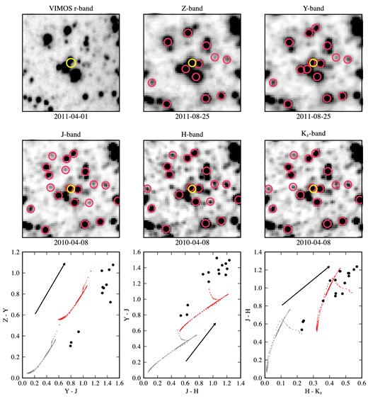
Postage stamps of CX0377 (Wu et al., in preparation), illustrating the high density of sources within 10 arcsec of the X-ray position plotted in yellow. The red circles correspond to the VVV sources detected in each band separately. We also plot three colour–colour diagrams (Z − Y versus Y − J, Y − J versus J − H, J − H versus H − Ks) with the VVV matches found in each case. We add reddened and un-reddened synthetic tracks of main-sequence stars, in red and grey, respectively, as well as a reddening vector (with E(B − V) = 1.53). The high number of possible matches is due to the very large uncertainties in the X-ray position. Many sources suffer from blending and they only become clearer in the Ks band (the seeing gets better in longer wavelengths). We also notice the non-detection of some objects in the given filters, despite their clear presence in the images. This is probably due to issues with the crowding and sky subtraction in the pipeline.
5.1 Quantifying the false alarm rate
The goal of this study is to quantify the false alarm rate when matching the GBS X-ray sources with NIR surveys of the bulge given the large stellar densities. Not only do we take into account the positional uncertainties of each GBS source, we also calculate a statistical false alarm probability (FAP) based on the brightness of the NIR match as well as its distance from the X-ray position. A final test is done taking into account the fact that for a given GBS source, more than one match is often detected, thus an FAP is evaluated for each match individually.
5.2 Random matching
In order to quantify the false alarm rate of our VVV matches, we generate a catalogue containing ∼40 000 random positions near the GBS source positions. In order to avoid duplicates, the sources in the generated catalogues are at least 10 arcsec away from each other and fall in regions with 0.5° < |b| < 3° and −3° < l < 4°. We cross-match those random positions with the positions of stars detected in VVV and search for their nearest NIR counterparts. Such a random test preserves the specific environments our GBS sources are detected in, and also carries with it any source detection biases the survey may have. In this way it self-calibrates and is preferred over analytic estimates based on stellar densities. In Fig. 8, we show a density map (in Ks mag versus distance) of the background field population of sources which could lead to false matches, and overplot in red dots the Ks-band magnitudes of each VVV closest match to the GBS sources against their separation from them. We notice that the counterparts of the GBS sources do not follow the same distribution as the generated sources, where the bulk of random sources fall within a defined region in the figure. This is an indication that in many cases (e.g. sources with Ks < 12), the VVV matches of the GBS are not random sources.
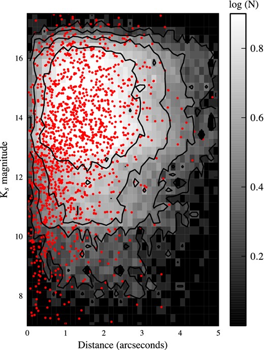
Density plot of the Ks-band magnitudes of the nearest VVV matches of ∼40 000 generated sources in the bulge against their distances to the corresponding sources. The grey-scale is a normalized logarithmic scale. The red dots correspond to the nearest VVV matches to the GBS sources. Sources brighter than 8th magnitude are not included in this figure because they are the main focus of the study carried out by Hynes et al. (2012).
We continued quantifying the false alarm rate by using this density map to create a cumulative FAP map as a function of the source's Ks-band magnitude and distance to it (see Fig. 9). The grey dots in Fig. 9 correspond to the GBS counterparts. It is important to remember that objects fainter than Ks ∼16 were not detected reliably, even if there is evidence for those sources in the VVV images (see Section 3.3). Therefore, the FAP distribution in the region above the black horizontal line in Fig. 9 is artificially low, due to the lack of detected sources. Only a handful of sources have matches fainter than Ks ∼ 16, but in this regime we extrapolate our FAP distribution for the GPS counterparts. Note that this analysis can be done in any filter and we illustrate it here in the Ks band since it has the best coverage and suffers from lower extinction and thus tends to have the highest source densities.
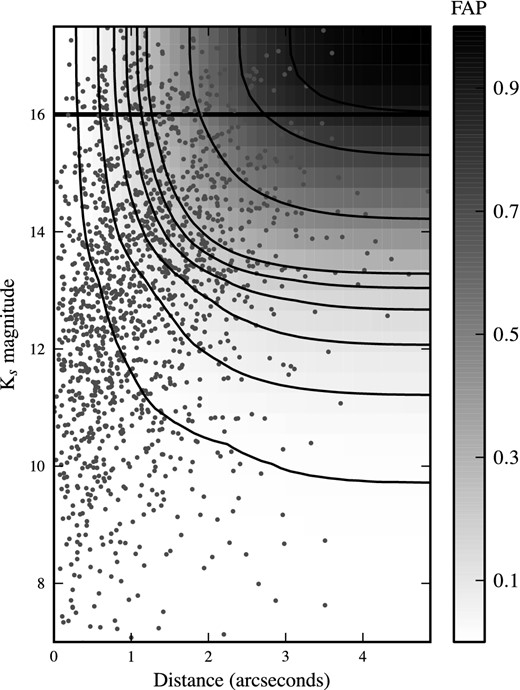
Cumulative distribution of the FAP of having the real VVV match. The contours indicate an FAP at 0.01, 0.05, 0.1, 0.15, 0.25, 0.5, 0.75 and 0.9. The grey dots correspond to the nearest VVV counterparts of the GBS sources. The FAP distribution in the region above the black horizontal line is artificially low, due to the lack of detected sources.
With such a cumulative distribution at hand, we calculate the FAP (FAPrandom) for each GBS counterpart by interpolating across both source magnitude and separation to find the FAP value for that counterpart. Therefore, each NIR match within R95 of a GBS source will have an associated FAP, which depends on its magnitude and distance to its NIR match and reflects the density of field sources near GBS sources. The FAPrandom obtained this way does not yet take into account the fact that multiple matches present themselves per source, nor the positional uncertainties of each GBS source. Therefore, we must calculate additional FAP based on those two criteria.
5.3 Positional uncertainties
5.4 Total FAP
We assign a final FAP (|${\rm FAP}_\mathrm{final}$|) to each viable matched source by taking into account the FAP calculated through the cross-matching of random sources in the GBS area with VVV and the FAP based on the positional uncertainties of the GBS sources: |${\rm FAP}_\mathrm{final} = {\rm FAP}_\mathrm{position} \times {\rm FAP}_\mathrm{random}$|. We show the distribution of |${\rm FAP}_\mathrm{final}$| in Fig. 10, where ∼90 per cent (1490 sources) of the GBS sources have a final FAP < 10 per cent and ∼79 per cent of them have a final FAP < 3 per cent. Even though 10 per cent remains a high value in terms of FAP, it nonetheless confirms that we are not dominated by false matches to field stars and that the NIR matches found for most of the GBS sources are genuine counterpart candidates. About ∼3 per cent of the sources in the VVV NIR Ks band catalogue did not have a valid Ks-band magnitude within R95, so they could not have a final FAP assigned to them.
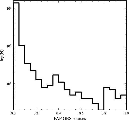
Total FAP distribution of the GBS sources. Around 90 per cent of the sources have a final FAP < 0.1 and ∼79 per cent have FAP < 0.03.
5.5 Multiple matches
Our |${\rm FAP}_\mathrm{final} = {\rm FAP}_\mathrm{position} \times {\rm FAP}_\mathrm{random}$| combines the fact that for larger source distances, FAP rate are higher due to field star contamination, but at the same time the probability that these are genuine matches is reduced. More than one match may be consistent with our GBS source position and the closest match is not necessarily the best match. In order to identify the most likely counterpart to the X-ray source (i.e. the match with the lowest |${\rm FAP}_\mathrm{final}$|), we repeat the same process of calculating |${\rm FAP}_\mathrm{position}$| and |${\rm FAP}_\mathrm{random}$| for all the NIR matches within R95 of the total positional uncertainty of the source. We show in Fig. 11 that typically, the GBS sources have two possible matches within R95. This value comes from the median of the distribution shown in Fig. 11.
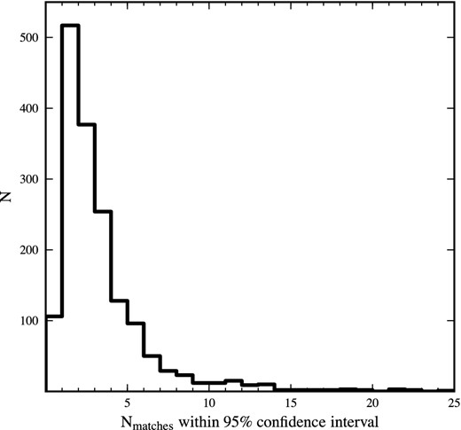
Number of VVV matches found in a 95 per cent confidence interval (R95) from each X-ray source. The median value of this distribution is 2, meaning that each GBS source had typically two potential NIR matches in its R95 positional error radius.
In Fig. 12, we show the |${\rm FAP}_\mathrm{final}$| for the nearest VVV matches (panel a), as well as the second (panel b), third (panel c) and fourth (panel d) closest matches within R95. We clearly see that the |${\rm FAP}_\mathrm{final}$| increases as we move further away from the X-ray position. This indicates that the closest match has the most likely chance of being a real match, since the fourth closest VVV match has a typical |${\rm FAP}_\mathrm{final}$| of 80 per cent. In addition, the number of sources with a fourth match within R95 decreases. Even though it is clear that the closest match is most likely to be the one with the lowest |${\rm FAP}_\mathrm{final}$|, we found that in 50 cases, the second closest match had a slightly lower |${\rm FAP}_\mathrm{final}$| than the nearest one. This only represents ∼3 per cent of the sources but it is important to note. In such cases, the distances between the closest and second closest matches are similar yet the second closest match is brighter than the nearest one, making it a statistically more likely real counterpart to the X-ray source.
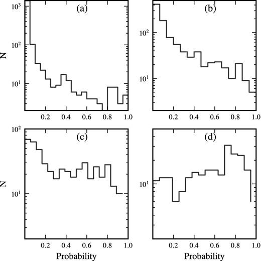
|${\rm FAP}_\mathrm{final}$| of four closest matches, within R95 of the X-ray position. Panels (a), (b), (c) and (d) correspond to the distributions of |${\rm FAP}_\mathrm{final}$| of the closest, the second closest, the third closest and the fourth closest matches to the X-ray position. The total number of sources clearly drops as we move away from the X-ray position.
To illustrate this, we consider CX0013 as an example. In this case, we find four matches within its R95 (see Fig. 13 and Table 3). As we move further away from the X-ray position, the final FAP does increase dramatically making the closest match the preferred choice. However, upon inspection of the images, we notice a very faint object even closer to the X-ray position. This source is too faint to make it into the NIR source catalogues considered in this study. This is an important reminder that despite our analysis, we must always consider the possibility of even fainter sources not detected in VVV. Our source table identifies the most likely counterpart among the detected sources in VVV, 2MASS and UKIDSS GPS.
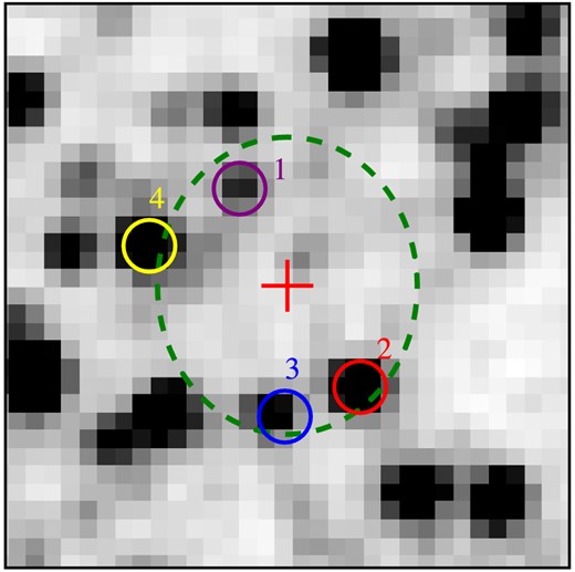
Positions of the four closest matches of CX0013 found within R95 in VVV. The red cross indicates the X-ray position and the large dashed green circle indicates the R95 boundary of 2.84 arcsec in this case. The table below provides information on their magnitudes and FAP.
Five closest VVV matches to CX0013.
| Source | Distance | Ks | |${\rm FAP}_\mathrm{final}$| |
|---|---|---|---|
| 1 | 2.07 | 15.60 | 0.069 |
| 2 | 2.40 | 14.36 | 0.138 |
| 3 | 2.50 | 15.38 | 0.188 |
| 4 | 2.75 | 14.02 | 0.349 |
| Source | Distance | Ks | |${\rm FAP}_\mathrm{final}$| |
|---|---|---|---|
| 1 | 2.07 | 15.60 | 0.069 |
| 2 | 2.40 | 14.36 | 0.138 |
| 3 | 2.50 | 15.38 | 0.188 |
| 4 | 2.75 | 14.02 | 0.349 |
5.6 Final table
To assist the characterization of the GBS source population, we provide in Table 4 the NIR positions, magnitudes and calculated Ks-band FAPfinal for all the detected sources within R95 of the GBS X-ray positions. Such a table presents a useful resource to anyone interested in studying the GBS sources, in particular at longer wavelengths and can be downloaded through the web version of this article. Here, we only show the results for the first 30 brightest sources as an example of the full table, which contains 4661 entries.
Table containing all NIR data and FAP of matches within R95.
| GBS source | RA GBS | Dec. GBS | RA NIR | Dec. NIR | Offset | J mag | J err | H mag | H err | K mag | K err | Survey | |${\rm FAP}_\mathrm{final}$| | Comments |
|---|---|---|---|---|---|---|---|---|---|---|---|---|---|---|
| 1 | 17 50 24.44 | −29 02 16.4 | 17 50 24.55 | −29 02 15.6 | 1.793 | 15.908 | 0.027 | 13.284 | 0.028 | 12.374 | 0.033 | 2MASS | 3.161e−02 | – |
| 2 | 17 37 28.39 | −29 08 02.0 | 17 37 28.39 | −29 08 02.1 | 0.034 | 13.633 | 0.056 | 12.257 | 0.054 | 11.187 | 0.059 | 2MASS | 2.851e−09 | (a) |
| 3 | 17 40 42.81 | −28 18 08.0 | 17 40 42.96 | −28 18 11.5 | 3.998 | 9.075 | 0.214 | 7.598 | 0.212 | 6.947 | 0.254 | 2MASS | 2.176e−02 | – |
| 4 | 17 39 31.22 | −29 09 52.8 | 17 39 31.22 | −29 09 53.3 | 0.515 | 7.209 | 0.001 | 6.566 | 0.003 | 6.384 | 0.004 | 2MASS | 1.369e−08 | (b) |
| 5 | 17 40 09.13 | −28 47 25.6 | 17 40 09.21 | −28 47 25.9 | 0.977 | 15.459 | 0.047 | 14.451 | 0.018 | 13.858 | 0.02 | VVV | 1.759e−03 | (c) |
| 6 | 17 44 45.78 | −27 13 44.5 | 17 44 45.77 | −27 13 44.4 | 0.112 | 7.054 | 0.057 | 6.843 | 0.051 | 6.507 | 0.055 | 2MASS | 8.455e−11 | (b) |
| 6 | 17 44 45.78 | −27 13 44.5 | 17 44 45.85 | −27 13 45.0 | 1.109 | – | – | – | – | 10.501 | 0.002 | VVV | 1.548e−03 | – |
| 6 | 17 44 45.78 | −27 13 44.5 | 17 44 45.70 | −27 13 45.1 | 1.302 | 10.927 | 0.001 | – | – | 10.46 | 0.002 | VVV | 3.104e−03 | – |
| 7 | 17 38 26.18 | −29 01 49.4 | 17 38 26.21 | −29 01 49.5 | 0.323 | 9.388 | 0.006 | 8.916 | 0.011 | 8.823 | 0.017 | 2MASS | 6.359e−09 | (b) |
| 8 | 17 35 08.28 | −29 29 57.9 | 17 35 08.24 | −29 29 58.2 | 0.556 | – | – | – | – | 10.665 | 0.002 | VVV | 7.200e−06 | – |
| 9 | 17 35 08.40 | −29 23 28.4 | 17 35 08.42 | −29 23 28.3 | 0.169 | 10.162 | 0.006 | 9.828 | – | 9.659 | 0.006 | 2MASS | 4.857e−09 | (b) |
| 10 | 17 36 29.04 | −29 10 28.8 | 17 36 29.06 | −29 10 29.1 | 0.470 | 7.967 | 0.019 | 7.464 | 0.021 | 7.264 | 0.025 | 2MASS | 3.453e−07 | (b) |
| 11 | 17 41 51.30 | −27 02 23.5 | 17 41 51.42 | −27 02 23.8 | 1.705 | 15.146 | 0.014 | 14.04 | 0.012 | 13.505 | 0.013 | VVV | 1.957e−02 | – |
| 12 | 17 43 47.24 | −31 40 25.2 | 17 43 47.26 | −31 40 25.2 | 0.411 | 6.998 | 0.001 | 6.364 | 0.001 | 6.165 | 0.001 | 2MASS | 3.020e−08 | (b) |
| 13 | 17 50 29.13 | −29 00 02.3 | 17 50 29.20 | −29 00 00.5 | 2.066 | – | – | – | – | 15.599 | – | VVV | 6.935e−02 | – |
| 13 | 17 50 29.13 | −29 00 02.3 | 17 50 29.03 | −29 00 04.3 | 2.402 | 16.587 | 0.11 | 14.92 | 0.076 | 14.363 | 0.074 | VVV | 1.380e−01 | – |
| 13 | 17 50 29.13 | −29 00 02.3 | 17 50 29.14 | −29 00 04.8 | 2.500 | 17.253 | 0.194 | – | – | 15.376 | 0.179 | VVV | 1.880e−01 | – |
| 13 | 17 50 29.13 | −29 00 02.3 | 17 50 29.33 | −29 00 01.6 | 2.745 | 16.203 | 0.078 | 14.58 | 0.056 | 14.02 | 0.055 | VVV | 3.349e−01 | – |
| 14 | 17 46 23.67 | −31 35 00.8 | 17 46 23.69 | −31 35 00.6 | 0.191 | 9.962 | 0.33 | 9.262 | – | 9.119 | – | 2MASS | 1.355e−09 | – |
| 15 | 17 46 46.17 | −25 52 17.5 | 17 46 46.25 | −25 52 17.5 | 0.948 | 16.198 | 0.23 | 15.571 | 0.409 | 15.392 | – | VVV | 1.381e−03 | – |
| 16 | 17 55 45.83 | −27 58 14.0 | 17 55 45.84 | −27 58 13.8 | 0.288 | 12.908 | – | 12.104 | – | 11.72 | 0.499 | 2MASS | 3.330e−07 | – |
| 16 | 17 55 45.83 | −27 58 14.0 | 17 55 45.84 | −27 58 15.8 | 1.843 | 15.269 | 0.017 | – | – | 14.036 | 0.036 | VVV | 4.314e−02 | – |
| 17 | 17 52 53.02 | −29 22 09.1 | 17 52 52.96 | −29 22 08.0 | 1.383 | – | – | 13.778 | – | 13.538 | – | VVV | 7.763e−03 | – |
| 17 | 17 52 53.02 | −29 22 09.1 | 17 52 53.14 | −29 22 09.4 | 1.631 | 12.437 | 0.036 | 11.27 | 0.031 | 10.893 | 0.069 | 2MASS | 1.124e−02 | – |
| 18 | 17 39 35.77 | −27 29 35.9 | 17 39 35.76 | −27 29 36.0 | 0.142 | 15.702 | 0.001 | 14.93 | 0.001 | 14.601 | 0.001 | VVV | 2.422e−08 | (c) |
| 19 | 17 49 54.57 | −29 43 35.4 | 17 49 54.53 | −29 43 35.8 | 0.745 | 11.989 | – | 10.432 | – | 9.93 | 0.046 | 2MASS | 5.201e−05 | – |
| 20 | 17 38 59.68 | −28 24 49.1 | 17 38 59.66 | −28 24 49.5 | 0.407 | 15.768 | 0.018 | 15.117 | 0.015 | 14.636 | 0.016 | VVV | 7.970e−06 | – |
| 21 | 17 41 33.76 | −28 40 33.8 | 17 41 33.79 | −28 40 34.5 | 0.890 | 17.284 | 0.093 | 16.849 | 0.055 | 16.447 | 0.058 | UKIDSS | 8.253e−04 | – |
| 22 | 17 45 54.02 | −31 15 03.4 | 17 45 54.01 | −31 15 03.2 | 0.146 | 10.27 | – | 9.619 | – | 9.472 | – | 2MASS | 1.725e−09 | – |
| 23 | 17 42 31.56 | −27 43 49.1 | 17 42 31.56 | −27 43 48.3 | 0.808 | 11.048 | 0.065 | 9.527 | 0.056 | 8.907 | 0.053 | 2MASS | 7.205e−05 | – |
| 24 | 17 48 49.51 | −30 01 09.9 | 17 48 49.50 | −30 01 10.3 | 0.368 | 10.947 | 0.001 | 10.217 | 0.002 | 9.965 | 0.002 | 2MASS | 3.882e−08 | – |
| 24 | 17 48 49.51 | −30 01 09.9 | 17 48 49.71 | −30 01 09.7 | 2.559 | – | – | 13.864 | 0.019 | 13.363 | 0.024 | VVV | 2.020e−01 | – |
| 25 | 17 45 02.78 | −31 59 35.0 | 17 45 02.77 | −31 59 34.5 | 0.704 | 10.175 | 0.023 | 9.719 | 0.039 | 9.584 | 0.059 | 2MASS | 3.018e−05 | (b) |
| 26 | 17 45 33.26 | −30 58 56.2 | 17 45 33.27 | −30 58 55.9 | 0.122 | 7.666 | 0.017 | 7.395 | 0.017 | 7.335 | 0.023 | 2MASS | 1.069e−10 | (b) |
| 27 | 17 36 52.83 | −28 48 41.6 | 17 36 52.83 | −28 48 41.4 | 0.130 | 11.621 | 0.022 | – | – | 10.524 | 0.03 | VVV | 2.664e−10 | (b)-Saturated |
| 28 | 17 39 46.98 | −27 18 09.5 | 17 39 47.01 | −27 18 08.9 | 0.680 | 14.658 | 0.002 | 14.009 | 0.002 | 13.711 | 0.002 | VVV | 1.213e−04 | (c) |
| 29 | 17 53 41.91 | −28 03 53.4 | 17 53 41.89 | −28 03 53.8 | 0.373 | 13.654 | 0.168 | 12.773 | 0.3 | 12.502 | 0.345 | 2MASS | 2.673e−06 | – |
| 30 | 17 49 20.62 | −30 18 31.8 | 17 49 20.55 | −30 18 32.4 | 1.045 | 16.618 | 0.039 | 15.697 | – | 15.369 | – | VVV | 2.219e−03 | – |
| 30 | 17 49 20.62 | −30 18 31.8 | 17 49 20.68 | −30 18 31.0 | 1.101 | 17.861 | 0.164 | 16.542 | 0.196 | 16.266 | 0.296 | VVV | 3.029e−03 | – |
6 DISCUSSION
6.1 Influence of the hardness of the X-ray sources
Since for most GBS sources, only a few counts are detected across the full 0.3 to 8 keV energy band, we have hardness ratios for the 164 brightest X-ray sources in GBS only. For the remaining GBS object, we can consider the energy range over which the sources were detected in. Therefore, they can be given, when available, a hardness classification: soft X-ray sources are detected in the 0.3–2.5 keV band, while hard X-ray sources are detected solely in the 2.5–8 keV band. We find that 327 sources are detected in the soft band, 444 are hard and the rest do not have a classification. In order to see if there is a correlation between the hardness of the X-ray sources, their NIR colours and the reddening towards the GBS fields, we plot a (J − Ks, Ks) colour–magnitude diagram of the closest VVV matches to the GBS sources (see Fig. 14). These sources are then colour-coded according to the X-ray hardness of the X-ray source, where red and green crosses correspond to hard and soft sources, respectively. We also add a reddening vector with E(B − V) = 1.8, since it corresponds to the typical extinction value towards the GBS region. Looking at the colour–magnitude diagram, we notice that soft sources are less affected by reddening than hard X-ray sources. This is an indication that the soft X-ray sources are more likely to be foreground objects whereas hard X-ray sources are probably reddened sources lying behind significant layers of extinction. Also most soft sources seem to have bright NIR matches, making them foreground sources and most probably the real matches. In order to confirm this result, we look at the |${\rm FAP}_\mathrm{final}$| values of the soft and hard sources. We find that 90 per cent of the soft sources have an |${\rm FAP}_\mathrm{final} <$| 3 per cent, whereas this is the case for only 68 per cent of the hard sources. This indicates that we have probably found the real (foreground) NIR counterparts to the soft GBS sources.
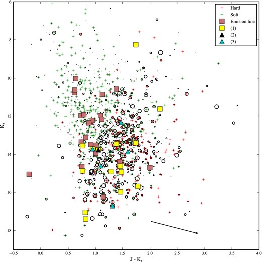
(Ks) versus (J − Ks) colour–magnitude diagram of the VVV matches with |${\rm FAP}_\mathrm{final}$| < 0.1. The size of the circle is proportionate to the value of the |${\rm FAP}_\mathrm{final}$| of the source. The larger the circle, the bigger the |${\rm FAP}_\mathrm{final}$|. The red and green crosses correspond to the hard and soft X-ray sources, respectively. The pink squares are Hα emission line sources (AGN, M-stars, RS CVns) and the yellow squares are accreting binaries (Torres et al. 2013), all confirmed via spectroscopy. The black triangle corresponds to CX0093, a CV confirmed by Ratti et al. (2013) and the cyan triangles correspond to the CVs studied in Britt et al. (2013). The black arrow indicates the reddening for an extinction value of E(B − V) = 1.8.
The combination of the NIR colours with the hardness of X-ray sources can provide additional information on the nature of the object beyond its proximity to the X-ray source. However, given the significant FAP for even the best matches, additional data are desired. Indeed, an optical component is a key part of the GBS strategy. This consists of both optical imaging as well as spectroscopy. Here, we briefly compare the NIR colour of some of these confirmed Hα emission line objects.
6.2 NIR colours of Hα emission line objects
In Fig. 14, we show in pink squares some of the confirmed Hα emission line sources in the GBS catalogue such as AGN, single M-stars and RS CVn systems. Also, Torres et al. (2013) have obtained spectra for several GBS sources and 23 objects show Hα emission in their spectra, as well as accretion signatures. These types of X-ray binaries are our principle science targets and are plotted in yellow squares. As can be seen, many Hα emission line objects fall in the region populated by the soft X-ray sources, possibly indicating that they are not bulge sources. We also notice that most X-ray binary systems occupy the same region as the hard X-ray sources. However, they do not occupy a very distinct region of the diagram, making the source classification difficult when using NIR colours alone. The black triangle corresponds to CX0093 (also known as CX0153), a CV studied by Ratti et al. (2013), and the cyan triangles are the CVs published by Britt et al. (2013).
6.3 Towards the identification of key GBS source classes
Despite the various studies of Galactic Centre X-ray sources using NIR photometry and spectroscopy (see Section 1), classifying objects on the basis on their colours alone is difficult. The Galactic Centre and bulge suffer from different amounts of extinction, which in itself varies on very small scales, greatly altering the colours. Therefore, strategies driven by a source's position in a colour–colour or colour–magnitude diagram cannot be directly employed in these environments even though such methods are highly effective at high Galactic latitudes.
In addition to the effects of reddening, the intrinsic colours of the sources expected in the GBS show great diversity. The key source types include LMXBs, CVs, UCXBs, RS CVn stars, W UMa and Be X-ray binaries. In the case of quiescent LMXBs, one may expect the companion stars to dominate the spectral energy distribution in the NIR. As these are typically late-type dwarfs, such objects may indeed have colours very similar to reddened field dwarfs. Comparison with theoretical colours of main-sequence and giant stars, as well as the correct reddening towards the line of sight of the X-ray source, can then help with the identification of potential NIR counterparts to the GBS sources. However, the presence of accretion continuum sources such as from accretion discs and jets will alter the colours. This diversity even among one subclass of, for example LMXBs, means that the NIR colours need complimentary constraints from other wavelength studies for a reliable classification of sources.
Previous work suggests that the NIR colours of CVs are similar to F–K main-sequence stars (Hoard et al. 2002). Since most CVs are foreground objects, they do not suffer from the same amount of reddening as potential bulge LMXBs. Note that this does not mean that their donor stars have spectral types of F–K as also in CVs accretion components will contribute. Knigge, Baraffe & Patterson (2011) also found that NIR colours of CVs were dominated by the donor star, except for systems close to the period minimum where contributions from the WD were beginning to be more significant. Indeed, the majority of these systems have optical spectra dominated by the WD (Gänsicke et al. 2009). Given their very low mass donors, the NIR colours of such systems thus no longer track a simple donor star sequence. It is also important to note that ∼20 per cent of CVs contain a magnetic WD (polars or intermediate polars). It has been found that they contribute towards a large fraction of the hard X-ray sources in the Galactic Centre (Muno et al. 2004; Hong 2012; Britt et al. 2013) since their X-ray luminosities are significantly higher than that of non-magnetic CVs. Luminosity ratios such as Lopt/LX can often be used as a crude discriminant between some of these source classes that otherwise may have similar NIR colours. Due to the fact the GBS is a shallow survey, with 2 ks exposures, most detected sources have typically less than 10 X-ray counts, leading to very poorly constrained X-ray fluxes. Another contribution to the large uncertainty of FX comes from the fact that the reddening towards the GBS X-ray sources is unknown. The VVV extinction maps yield a maximum limit to AKs, making it difficult to determine the actual X-ray flux of our sources. For this reason, we are unable to calculate reliable FX/FNIR in order to identify key GBS source classes.
RS CVn stars, a type of close detached binary stars, are known to be variable due to cool stellar spots present on the surfaces. A good way to select them is by exploiting the NIR variability information which is now available in VVV and which will be the main topic of a future paper.
The work presented here allows us to prioritize those with lowest |${\rm FAP}_\mathrm{final}$| for spectroscopic or photometric follow-up and also assess the impact of false matches. The FAP study is most reliable in the NIR (mainly in the Ks band) since we can probe through the dust and detect more bulge sources. With the final table presented in this study, which contains the most likely NIR counterparts to the GBS X-ray sources, we are now able to move on to the next stage of the GBS strategy, which is to use optical photometric and variability data to select the objects for spectroscopic follow-up. This has been demonstrated with the results found by Torres et al. (2013), where key GBS source classes have been identified via spectroscopy. The addition of optical data will enable us to disentangle the effects of reddening towards the GBS fields and separate the field CVs from the bulge LMXBs. The NIR variability information provided via VVV in the Ks band will also help us in selecting those viable counterparts that show evidence for variability, as would be expected for the majority of our objects. True secure classification, however, is best achieved through spectroscopy (Torres et al. 2013; Wu et al., in preparation).
7 CONCLUSION
We exploited three NIR surveys of the Galactic bulge to search for the NIR counterparts of the GBS X-ray sources. We found that VVV was the most uniform survey, in terms of coverage and depth. We exploit the NIR data, along with the X-ray information, in order to find the NIR counterparts of the Chandra sources. We quantify the false alarm rate of finding the real matches by calculating FAP for each source, taking into account their NIR magnitudes, distances to their matches, positional uncertainties and the multiple matches around each GBS object. We present these findings here in the form of a large data table (see Table 4 for a subset of the final version available online) that will be a useful resource for follow-up studies of the GBS sources. We find that ∼90 per cent of the GBS sources have an |${\rm FAP}_\mathrm{final}$| < 10 per cent and ∼79 per cent of them have an |${\rm FAP}_\mathrm{final}$| < 3 per cent. This indicates that we have found the NIR counterpart of more than half of the GBS sources. We have shown that there are typically two NIR matches within R95 of the X-ray position but at least one of those matches is very likely to be the real counterpart.
While spectroscopy ultimately is a superior way of classifying key sources, such as the bulge population of X-ray binaries, the ability to select candidates by using astronomical surveys and their photometric properties is crucial (Motch, Michel & Pineau 2009; Hynes 2010). The NIR photometric data discussed here are able to probe through the dust and surveys such as VVV now have the spatial resolution to resolve these environments adequately. Our results can now be used in concert with data of the GBS region at other wavelengths, in order to disentangle the effects of reddening. This will lead to a more tailored target follow-up strategy.
SG acknowledges support through a Warwick Postgraduate Research Scholarship. DS acknowledges support from STFC through an Advanced Fellowship (PP/D005914/1) as well as grant ST/I001719/1. RIH and CTB acknowledge support from the National Science Foundation under Grant no. AST-0908789. We gratefully acknowledge use of data from the ESO Public Survey programme ID 179.B-2002 taken with the VISTA telescope and data products from CASU. We warmly thank D. Minniti and P. Lucas for early access to the VVV data, as well as O. Gonzalez early access to his calculated reddening values. We are grateful for all the help provided by R. Saito and M. Irwin with the access and reduction of the CASU data.
The data can be found on http://surveys.roe.ac.uk/wsa/.
We downloaded the VVV images and catalogues from http://apm49.ast.cam.ac.uk/vistasp/imgquery/search.
http://cxc.harvard.edu/cal/ASPECT/celmon/ – Note that we consider the ACIS-S value since it is the best determined one, with most observations taken into account for its study. This is a spacecraft correction and should not depend on the instruments on board.
For more information on the photometric systems, see http://apm49.ast.cam.ac.uk/surveys-projects/vista/technical/photometric-properties.
The values were given by Stefano Rubele and Leo Girardi, members of the VVV team.
REFERENCES
SUPPORTING INFORMATION
Additional Supporting Information may be found in the online version of this article:
Table 4. Table containing all NIR data and FAP of matches within R95.
Please note: Oxford University Press is not responsible for the content or functionality of any supporting materials supplied by the authors. Any queries (other than missing material) should be directed to the corresponding author for the article.
