


ABSTRACT
Large surveys for Lyα emitting (LAE) galaxies have been proposed as a new method for measuring clustering of the galaxy population at high redshift with the goal of determining cosmological parameters. However, Lyα radiative transfer effects may modify the observed clustering of LAE galaxies in a way that mimics gravitational effects, potentially reducing the precision of cosmological constraints. We investigate the impact of Lyα radiative transfer effects on the observed clustering of LAE galaxies. In particular, we focus on the effects of the intergalactic medium velocity gradients, local density within the environment of an LAE galaxy and ionizing background fluctuations. For example, the effect of the linear redshift-space distortion on the power spectrum of LAE galaxies is potentially degenerate with Lyα radiative transfer effects owing to the dependence of observed flux on intergalactic medium velocity gradients. In this paper, we show that the three-point function (bispectrum) can distinguish between gravitational and non-gravitational effects, and thus breaks these degeneracies, making it possible to recover cosmological parameters from LAE galaxy surveys. Constraints on the angular diameter distance and Hubble expansion rate are independent of Lyα radiative transfer degeneracies; however, they incur slight reductions in their constraining power resulting from the overall reduction of the signal-to-noise due to the Lyα radiative transfer effects. Combining the power spectrum and bispectrum measurements provides improved constraints on the angular diameter distance and Hubble expansion rate.
1 INTRODUCTION
For the past three decades, galaxy redshift surveys have served as the traditional method for constraining cosmological parameters such as the matter density of the universe and the equation of state of dark energy, by measuring the clustering of galaxies. These have been restricted to z < 1 due to the increasingly fainter galaxy magnitudes and larger required cosmic volumes, which render spectroscopy of large numbers of photometrically selected early-type galaxies plausible only at such low redshifts. Recently, the WiggleZ collaboration has pushed galaxy clustering work to z ∼ 1 using emission lines from star-forming galaxies (Blake et al. 2011a,b,c, 2012).
Lyα emitting (LAE) galaxies are detectable out to high redshift (Iye et al. 2006; Kashikawa et al. 2006; Lehnert et al. 2010; Ouchi et al. 2010), due to their strong line emission. Indeed over the previous few years, the number of detected LAE sources has steadily grown and the sample sizes of LAE galaxies have reached sufficient size for clustering studies (Gawiser et al. 2007; Kovač et al. 2007; Orsi et al. 2008; Guaita et al. 2010; Ouchi et al. 2010).
While the existing samples of LAE galaxies are still too small for cosmological purposes, the rate of detection of these LAE galaxies will significantly improve with the upcoming Hobby–Eberly Telescope Dark Energy Experiment (HETDEX; Hill et al. 2004, 2008), whose aim is to spectroscopically measure the redshifts of 800 000 LAE galaxies in the redshift range 1.9 ≤ z ≤ 3.5 (Hill et al. 2004, 2008) with the total sky coverage of 420 square degrees and the total volume coverage of 10 Gpc3. This survey is specifically designed to use the clustering of LAE galaxies to make the precise measurement of the distance scales, both the angular diameter distance (DA) and the Hubble rate (H), as a function of z out to z ∼ 3.
In order for us to use the clustering of LAE galaxies to measure the distance scales, we must understand how the clustering of LAE galaxies is related to the underlying matter distribution. Simulations by Zheng et al. (2010, 2011) and Laursen, Sommer-Larsen & Razoumov (2011) have investigated the radiative transfer effects on the Lyα emission of LAE galaxies both within the circumgalactic environment around the halo and from the resonant scattering of diffuse neutral hydrogen in the intergalactic medium (IGM). Of particular interest is the clustering of the LAE galaxies: Zheng et al. (2011) find that line-of-sight gradients in the peculiar velocity of LAE galaxies could lead to an observed reduction in the line-of-sight clustering amplitude of the galaxies, counteracting the strength of the typical Kaiser effect (Kaiser 1987) caused by gravitation. Conversely, the clustering of LAE galaxies transverse to the line of sight is found to be significantly boosted by the Lyα radiative transfer effects. In addition to the local effects of peculiar velocity gradients, the transmission of the Lyα emission line of LAE galaxies through the diffuse IGM could also be affected by fluctuations in the UV ionizing background and to changes in the neutral hydrogen fraction associated with changes in the density around the local environment.
To understand these effects, Zheng et al. (2011) and Wyithe & Dijkstra (2011) have derived analytic models to describe the observed modifications of the power spectrum of LAE galaxies. Both derive quantities that directly relate to the non-gravitational effects expected from the Lyα radiative effects. Wyithe & Dijkstra (2011) use this model to study the expected recovery of both cosmological and Lyα radiative transfer parameters from a survey corresponding to HETDEX. They find that some cosmological parameters derived only from the power spectrum are degenerate with the Lyα radiative transfer effects, and that this has direct consequences for the accuracy with which cosmological parameters can be recovered from the LAE galaxy power spectrum. Prior knowledge of the magnitude of the radiative transfer effects can improve the recovery of the cosmological constraints.
In this paper, we further investigate the effects of non-gravitational LAE clustering on the recovery of cosmological parameters. We extend and improve the linear theory work of Wyithe & Dijkstra (2011) by including the three-point correlation function (bispectrum) and by combining with the power spectrum, to break the first-order degeneracies of the Lyα radiative transfer effects and cosmological parameters. To calculate the bispectrum, we use a next-to-leading-order Eulerian perturbation theory approach (Bernardeau et al. 2002 and references within), and derive expressions valid into the mildly non-linear regime. We also derive higher order expressions for the Lyα radiative transfer effects, including the higher order effects of redshift-space distortions. We then study how well a joint analysis of the power spectrum and the bispectrum can break the cosmological and radiative transfer degeneracies. We provide the expected constraints on cosmological parameters through the application of Fisher matrices, with specific reference to the HETDEX survey.
This paper is set out as follows. In Section 2, we outline the degeneracies between cosmological and Lyα radiative transfer parameters, and in Section 3, we perform a Fisher matrix analysis of the LAE galaxy power spectrum. In Section 4, we outline and describe existing Eulerian perturbation theory expressions and provide the derivation of higher order corrections for the Lyα radiative transfer effects, in order to construct both a bispectrum and a reduced bispectrum model. In Sections 5 and 6, we perform Fisher matrix analyses of the reduced bispectrum alone, and a combined power spectrum and bispectrum in order to provide cosmological parameter estimates. We finish with our summary and final remarks in Section 7. In our numerical calculations, we consider the standard set of cosmological parameters (Komatsu et al. 2011), with Ωm = 0.275, ΩΛ = 0.725, Ωb = 0.0458, ns = 0.968, h = 0.702 and σ8 = 0.816.
2 CLUSTERING OF Lyα EMITTERS
In this section, we summarize the linear theory clustering of LAE galaxies. For a galaxy redshift survey, one can write a simple expression relating the power spectrum of galaxies to the underlying matter distribution. However, for LAE galaxies, Zheng et al. (2011) and Wyithe & Dijkstra (2011) show that Lyα radiative transfer effects modify this relationship.
2.1 Galaxy power spectrum
2.2 LAE power spectrum
Lyα radiative transfer effects potentially modify the power spectrum of LAE galaxies away from the standard galaxy description (equation 1). This arises because the observed number density of Lyα galaxies at a fixed observed flux depends on how many Lyα photons escape to observers. Thus, the observed density of galaxies can be modified by the local environment nearby the Lyα galaxies.
Equation (12) contains the main contributing terms of Zheng et al. (2011). However, we do not include the transverse line-of-sight velocity gradient or the density gradient (as provided by Zheng et al. 2011). As shown in Zheng et al. (2011), the effect of the density gradient adds additional scale-dependent terms to the expression for the clustering of LAE galaxies on small scales. In this work, we are working at much larger scales, and so can ignore this scale dependence and allow the density-gradient terms to be absorbed into the existing parameters of equation (12).
The inclusion of Lyα radiative transfer effects introduces degeneracies between the cosmological parameters and Lyα radiative transfer parameters. In particular, from equation (12), we note the degeneracy between the growth rate of structure, f, and the line-of-sight peculiar velocity radiative transfer effect, Cv. Additionally, the galaxy bias, b1, is degenerate with the local environment density, Cρ, and the fluctuations in the ionizing background, CΓ.
Now, the problem is clear: while equation (13) has the same structure as equation (2), the meaning of each parameter is different. The correspondence is |$b_1\rightarrow \tilde{b}_1$| and |$\beta \rightarrow \tilde{\beta }(1-C_v)$|, which shows the parameter degeneracy. In the next section, we illustrate the resulting effect of radiative transfer parameters on the potential cosmological constraints.
3 COSMOLOGICAL CONSTRAINTS BASED ON THE LINEAR LAE GALAXY POWER SPECTRUM
We focus our attention on a survey like HETDEX, for which we assume the linear galaxy bias to be b1 = 2.2. We generate constraints assuming measurement of one redshift bin at the mid-point of the HETDEX redshift range, zmin = 1.9 and zmax = 3.5. At this redshift we have f = 0.972 for the growth rate of structure. We assume that HETDEX will detect 800 000 LAE galaxies in a total survey area of 420 square degrees. We restrict our analysis to the weakly non-linear regime, selecting a maximum wavenumber, kmax = 0.3 h Mpc−1.
To investigate the degeneracies due to Lyα radiative transfer parameters, we consider recovery of cosmological parameters from three power spectra:
the galaxy power spectrum given by equation (2),
a fiducial LAE power spectrum given by equation (13) with the fiducial values of radiative transfer parameters set to vanish, i.e. |$C_\Gamma =C_\rho =C_v=0$| (but these radiative transfer parameters are marginalized over) and
an LAE power spectrum given by equation (13) with the fiducial values of radiative transfer parameters set to some indicative values.
3.1 Galaxy power spectrum
For the galaxy power spectrum given by equation (2), the galaxy bias is completely degenerate with the amplitude of the power spectrum (σ8). Furthermore, one cannot directly measure the growth rate of structure, f, but only the parameter β. We show later that by considering the bispectrum, one can directly probe f.
The cosmological parameters we determine from this model are therefore the overall amplitude [ln(A)], the linear redshift-space distortion parameter [β], and the two distance measurements given by the angular diameter distance [ln(DA)] and the Hubble rate [ln(H)]. The information on the galaxy bias is factored into the linear redshift-space distortion parameter and we redefine the amplitude to include galaxy bias. The constrains for β as well as ln(DA) and ln(H) represent the best case scenario for how accurately we can recover the cosmological parameters from a galaxy power spectrum analysis.
In Table 1, we provide the 1σ constraints on β, and the two distance scales, DA and H. For a galaxy redshift survey with HETDEX-like survey parameters, the expected uncertainty on the linear redshift-space distortion, β, is 0.021 (4.8 per cent), on the angular diameter distance it is 1.1 per cent and on the Hubble rate it is 1.3 per cent. Our distance constraints for the above model are consistent with the results of Shoji, Jeong & Komatsu (2009).
The 1σ constraints for the linear redshift-space distortion parameter, β, the angular diameter distance, ln(DA), and the Hubble rate, ln(H), for a galaxy redshift survey with HETDEX-like survey parameters. The other model parameters are marginalized over, but no Lyα radiative transfer effects are included, i.e. the power spectrum is given by equation (2).
| Parameter | Marginalization | PS | |
|---|---|---|---|
| 1σ (per cent) | |||
| β | ln (A) | 0.0091 (2.06) | |
| β | ln(A), ln(DA), ln(H) | 0.0213 (4.82) | |
| ln(DA) | ln (A), β, ln (H) | 0.0110 (1.10) | |
| ln (H) | ln(A), β, ln(DA) | 0.0132 (1.32) |
| Parameter | Marginalization | PS | |
|---|---|---|---|
| 1σ (per cent) | |||
| β | ln (A) | 0.0091 (2.06) | |
| β | ln(A), ln(DA), ln(H) | 0.0213 (4.82) | |
| ln(DA) | ln (A), β, ln (H) | 0.0110 (1.10) | |
| ln (H) | ln(A), β, ln(DA) | 0.0132 (1.32) |
Of particular interest for cosmological analyses is the two-dimensional joint constraints on the two distance measures, ln(DA) and ln (H). In the left-hand panel of Fig. 1, we show the 1σ and 2σ joint constraints on ln(DA) and ln (H), which give the baseline for comparison with the recovery of the cosmological distance parameters for DA and H for the remainder of this work.
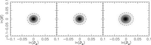
Two-dimensional marginalized joint distribution for the two cosmological distance scales: the angular diameter distance (DA) and the Hubble rate (H). (Left) a typical galaxy redshift survey (no Lyα effects; no marginalization over Cv), (middle) a fiducial LAE galaxy redshift survey (the fiducial values of the Lyα radiative transfer parameters set to vanish; marginalized over Cv) and (right) an LAE galaxy redshift survey including the first-order Lyα radiative transfer effects given by CΓ = 0.05, Cρ = −0.39 and Cv = 0.11. The error ellipse is slightly bigger for this case because the effective bias of LAE galaxies, |$\tilde{b}_1=1.9$|, is about 15 per cent smaller than the fiducial value, b1 = 2.2, reducing the amplitude of the power spectrum relative to the shot noise. The solid and dashed curves show the 1σ and 2σ constraints generated from the likelihood distribution, respectively. Scale selected to aid comparison with Fig. 7.
3.2 Fiducial LAE galaxy power spectrum
We model the LAE galaxy power spectrum using equation (13). In our fiducial case, we set all Lyα radiative transfer coefficients to zero, i.e. |$\tilde{b}_{1} = b_{1}$|, |$\tilde{\beta } = \beta$| and Cv = 0. Although we set the Lyα radiative transfer effects to zero, we still marginalize over the possible existence of Cv in this case.
The amplitude of the power spectrum is completely degenerate with the modified galaxy bias, and so we can redefine the amplitude to include |$\tilde{b}_{1}$|. The LAE galaxy power spectrum includes Cv, the Lyα radiative transfer effect associated with the line-of-sight peculiar velocity gradient. Hence, for the LAE galaxy power spectrum, the model contains five parameters, ln (A), |$\tilde{\beta }$|, Cv, ln (DA) and ln (H). The linear redshift-space distortion parameter, |$\tilde{\beta }$|, and the radiative transfer effect, Cv, are completely degenerate; however, with the addition of priors on Cv, one can break the degeneracy and improve the constraints on the linear distortion parameter, |$\tilde{\beta }$| (Wyithe & Dijkstra 2011).
In Table 2, we provide the resulting 1σ constraints on the linear redshift-space distortion parameter, |$\tilde{\beta }$|, as well as the distance constraints, marginalized over the remaining model parameters including Cv. The columns from left to right in Table 2 consider priors added to Cv, essentially perfect knowledge of Cv, |$\sigma _{C_{v}} = 0.0001$|,2|$\sigma _{C_{v}} = 0.01$|, |$\sigma _{C_{v}} = 0.1$| and |$\sigma _{C_{v}} = 0.5$|. The inclusion of Cv into the model significantly impacts the recovery of the linear redshift-space distortion parameter, |$\tilde{\beta }$|, whereas the distance constraints remain unaffected by the marginalization over the radiative transfer effects. This differs from Wyithe & Dijkstra (2011) where the inclusion of scale-dependent ionizing background fluctuations leads to reduced distance constraints.
The 1σ constraints for |$\tilde{\beta }$|, ln (DA) and ln (H) for our fiducial LAE galaxy redshift survey (the fiducial values of the Lyα radiative transfer parameters set to vanish) marginalized over remaining model parameters shown in the second column. We compare varying priors added to the radiative transfer parameter, Cv, which suffers from a large degeneracy with |$\tilde{\beta }$|. The power spectrum model is given by equation (13).
| Parameter | Marginalization | No priors on Cv | Perfect knowledge | |$\sigma _{C_{v}} = 0.01$| | |$\sigma _{C_{v}} = 0.1$| | |$\sigma _{C_{v}} = 0.5$| |
|---|---|---|---|---|---|---|
| 1σ (per cent) | 1σ (per cent) | 1σ (per cent) | 1σ (per cent) | 1σ (per cent) | ||
| |$\tilde{\beta }$| | ln (A),Cv | – | 0.0091 (2.06) | 0.0101 (2.29) | 0.0451 (10.21) | 0.2211 (50.04) |
| |$\tilde{\beta }$| | ln(A), ln(DA), ln(H),Cv | – | 0.0213 (4.82) | 0.0218 (4.93) | 0.0491 (11.11) | 0.2220 (50.24) |
| ln(DA) | |${\rm ln}(A),\tilde{\beta },{\rm ln}(H)$|,Cv | 0.0110 (1.10) | 0.0110 (1.10) | 0.0110 (1.10) | 0.0110 (1.10) | 0.0110 (1.10) |
| ln (H) | |${\rm ln}(A),\tilde{\beta },{\rm ln}(D_{{\rm A}})$|,Cv | 0.0132 (1.32) | 0.0132 (1.32) | 0.0132 (1.32) | 0.0132 (1.32) | 0.0132 (1.32) |
With sufficiently tight priors on Cv, the constraints on |$\tilde{\beta }$| approach the results given in the previous section, as expected. If we have a poor understanding of Cv, however, the ability to recover |$\tilde{\beta }$| drops by an order of magnitude. See the left-hand panel of Fig. 2 for a graphical representation of the effect of the priors.
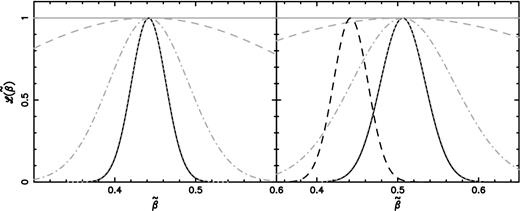
One-dimensional marginalized likelihood distributions for the linear redshift-space distortion parameter (|$\tilde{\beta }$|) generated from (left) the fiducial LAE galaxy power spectrum (no Lyα effects, but marginalized over Cv) and ( right) an LAE galaxy power spectrum including Lyα radiative transfer effects (CΓ = 0.05, Cρ = −0.39 and Cv = 0.11). The resultant offset in |$\tilde{\beta }$| in the LAE galaxy power spectrum (right-hand panel) is due to the modified bias because of the included Lyα radiative transfer effects. The various curves denote different priors added to Cv and are as follows, black solid: perfect knowledge (|$\sigma _{C_{v}} = 0.0001$|), grey dotted: |$\sigma _{C_{v}} = 0.01$|, grey dot–dashed: |$\sigma _{C_{v}} = 0.1$|, grey dashed: |$\sigma _{C_{v}} = 0.5$| and grey solid: no priors added. In the right-hand panel, the black dashed offset curve is the comparison to the case corresponding to perfect knowledge of Cv from the fiducial LAE galaxy power spectrum (black solid curve, left-hand panel).
On the other hand, the distance constraints are unaffected by the degeneracy between |$\tilde{\beta }$| and Cv. (Compare the middle panel of Fig. 1 with the left-hand panel.) This is because β and Cv enter into the power spectrum in the same way: as far as the distance scales are concerned, it makes no difference whether one marginalizes over β in equation (2) or |$\tilde{\beta }(1-C_v)$| in equation (13).
3.3 LAE galaxy power spectrum
Wyithe & Dijkstra (2011) show that the magnitude of the Lyα radiative transfer parameters varies significantly depending on the LAE model considered. In particular, the magnitude of the effect is significantly larger in the absence of a galactic outflow, so that the absorption is dominated by infalling IGM. For illustration we consider this ‘infall’ model with an escape fraction of 10 per cent, as this is the model with the largest magnitude Lyα radiative transfer effects. Hence, when we include the radiative transfer effects into our model, we set CΓ = 0.05, Cρ = −0.39 and Cv = 0.11 in equation (13).
In Table 3, we provide estimates for the recovery of cosmological parameters when we include the radiative transfer effects. The linear bias is modified from its fiducial value of b1 = 2.2 to |$\tilde{b}_{1} = 1.9$|, acting to reduce the observed clustering of LAE galaxies. As the level of the shot noise is the same, a reduced effective bias implies a lower signal-to-noise for measuring the power spectrum of LAE galaxies. As a result, the expected constraints on the angular diameter distance and the Hubble rate are worse than the previous two cases. One can see this clearly in the right-hand panel of Fig. 1.
Same as Table 1, but for the LAE galaxy redshift survey including first-order Lyα radiative transfer effects, CΓ = 0.05, Cρ = −0.39 and Cv = 0.11.
| Parameter | Marginalization | No priors on Cv | Perfect knowledge | |$\sigma _{C_{v}} = 0.01$| | |$\sigma _{C_{v}} = 0.1$| | |$\sigma _{C_{v}} = 0.5$| | |
|---|---|---|---|---|---|---|---|
| 1σ (per cent) | 1σ (per cent) | 1σ (per cent) | 1σ (per cent) | 1σ (per cent) | |||
| |$\tilde{\beta }$| | ln (A),Cv | – | 0.0121 (2.39) | 0.0134 (2.65) | 0.0582 (11.49) | 0.2847 (56.23) | |
| |$\tilde{\beta }$| | ln(A), ln(DA), ln(H),Cv | – | 0.0278 (5.49) | 0.0283 (5.59) | 0.0633 (12.50) | 0.2858 (56.45) | |
| ln(DA) | |${\rm ln}(A),\tilde{\beta },{\rm ln}(H)$|,Cv | 0.0128 (1.28) | 0.0128 (1.28) | 0.0128 (1.28) | 0.0128 (1.28) | 0.0128 (1.28) | |
| ln (H) | |${\rm ln}(A),\tilde{\beta },{\rm ln}(D_{{\rm A}})$|,Cv | 0.0151 (1.51) | 0.0151 (1.51) | 0.0151 (1.51) | 0.0151 (1.51) | 0.0151 (1.51) |
The same is true for |$\tilde{\beta }$|: due to a smaller effective bias, the fractional precision by which we can determine |$\tilde{\beta }$| is slightly worse than the previous cases. (One can see this by comparing the rows of ‘β’ in Tables 2 and 3.) Note also that, as the fiducial value of |$\tilde{b}_1$| is different due to the radiative transfer parameters, the fiducial value of |$\tilde{\beta }=f/\tilde{b}_1$| is also different.
In Fig. 2, we show the one-dimensional likelihood distributions for |$\tilde{\beta }$| for both the fiducial LAE galaxy model (left-hand panel) and the LAE galaxy model (with Lyα effects; right-hand panel). As already described in the previous section, the recovery of |$\tilde{\beta }$| from these models is highly sensitive to the priors on Cv, with marginal improvement on the priors breaking the degeneracy between |$\tilde{\beta }$| and Cv. In the right-hand panel, we compare the likelihood distribution for the case of perfect knowledge of Cv for the fiducial LAE galaxy model (the dashed line) to the LAE galaxy model (the solid line), showing the degree of offset that the Lyα radiative transfer parameters have on the fiducial value of |$\tilde{\beta }$|.
Thus, the inclusion of the Lyα radiative transfer parameters impacts the recovery of cosmological constraints, most notably the growth rate of structure f through the recovery of the linear redshift-space distortion parameter |$\tilde{\beta }$|. Unless we have good prior knowledge of the value of Cv, it seems hopeless to determine |$\tilde{\beta }$| with any precision. Fortunately, one can break the degeneracy between |$\tilde{\beta }$| and Cv by including the three-point function (bispectrum), as we shall show next.
4 BISPECTRUM AND NON-LINEAR CLUSTERING OF LAE GALAXIES
However, non-linear gravitational evolution of density fields, and non-linear gravitational and non-gravitational evolution of galaxy bias make the observed galaxy density fields non-Gaussian. As a result, the observed bispectrum does not vanish, providing information regarding non-linear evolution of density fields.
In the previous section, we have considered the linear theory power spectrum model for the LAE galaxy population. Structure formation is inherently a non-linear process, and by considering the true non-linear galaxy power spectrum one would expect to increase the constraining power. However, the non-linear power spectrum alone will not achieve this, due to the additional parameters required to fully describe it. Hence, the simple linear LAE galaxy power spectrum is preferred instead of the increased model complexity provided by the non-linear LAE galaxy power spectrum. On the other hand, additional information on large scales may be contained in the non-Gaussianity associated with structure formation.
We use this information to break the degeneracy between cosmological parameters and Lyα radiative transfer parameters. There are three effects: (1) gravitational evolution of matter density fields, (2) gravitational and non-gravitational evolution of galaxy formation (captured by galaxy bias), and (3) non-gravitational Lyα radiative transfer effects.
4.1 Eulerian perturbation theory
First, we summarize the non-linear gravitational evolution of density fields. Specifically, we apply standard Eulerian perturbation theory (Bernardeau et al. 2002 and references within) which, at larger redshifts, has been shown to describe the power spectrum measured from N-body simulations accurately (Jeong & Komatsu 2006).
4.2 Galaxy bias
Galaxies are biased tracers of the underlying dark matter density field (Kaiser 1984). Pushing into the weakly non-linear regime, we anticipate contributions from both the linear and non-linear mapping of galaxies to the dark matter field.
The bias of galaxies differs from population to population, and their exact value depends on the underlying galaxy formation processes. Typically we expect a scale-dependent bias relating the clustering of the galaxies to the underlying matter density on small scales, but on large scales we expect the bias to be scale independent.
4.3 LAE kernel expressions
Equations (28) and (29) contain the first- and second-order Lyα radiative transfer coefficients. In Appendix A, we derive the explicit expressions for the first-order Lyα radiative transfer coefficients, and use the same basic ideas to also derive the second-order coefficients.
4.4 LAE bispectrum and reduced bispectrum
The bispectrum in redshift space depends on six variables: three wavenumbers, k1, k2 and k3, giving the sides of a triangle, and the cosines of the angles that these three vectors make with the line-of-sight direction, μ1, μ2 and μ3. However, due to the triangular condition, these six variables are not all independent. Instead, the bispectrum can be written as a function of five independent variables (Scoccimarro, Couchman & Frieman 1999; Smith, Sheth & Scoccimarro 2008): three parameters [k1, k2 and the angle between them, cos(θ12)] define the shape of the triangle and the remaining two parameters (μ1 and φ) define the orientation of the triangles with respect to the line of sight.
4.5 Fisher matrix
Before generating the expected cosmological constraints using the Fisher matrix, let us first summarize the model parameters characterizing the higher order (non-linear) terms.
It is important to note that, unlike the previous work which simply multiplies the real-space bispectrum by the linear redshift distortion factors (Scoccimarro et al. 1999; Sefusatti et al. 2006; Sefusatti & Komatsu 2007), we include the full wavenumber dependence of the redshift-space distortion up to the second order. By including the full second-order redshift-space distortion, we gain additional information which helps to further break the degeneracies between the cosmological information and the radiative transfer effects, especially those associated with the velocity gradient.
In our model, we choose to keep the second-order effect due to the peculiar velocity gradient (Cvv) separate, as this has the potential to be degenerate with the growth rate of structure, f. Additionally, |$\tilde{C}$|, which contains the linear-order effects with respect to the peculiar velocity gradient, can also become degenerate with f. We note that setting the Lyα radiative transfer effects to zero reduces equation (37) to the typical second-order redshift-space galaxy kernel, as required.
5 CONSTRAINTS FROM THE REDUCED BISPECTRUM ALONE
In Section 3, we show that the growth rate of structure, f (or |$\tilde{\beta }$|), is completely degenerate with the Lyα radiative transfer effect due to the velocity gradient, Cv, as long as we rely only on the power spectrum.
However, the bispectrum provides additional constraining power that can be used to break the degeneracy between the growth rate of structure, f, the linear galaxy bias, |$\tilde{b}_{1}$|, and Cv. This is because non-linear structure formation such as the collapse on to filaments produces non-Gaussianity which is measurable only through the bispectrum (and higher order moments). For example, one needs information of the bispectrum in order to reproduce the ‘cosmic web,’ the filamentary structures in the universe. The power spectrum cannot distinguish between the distribution with random phases and that with the filamentary structures, as it is sensitive only to the amplitude of the fluctuations. As a result, the bispectrum can distinguish between the structures caused by gravitational and non-gravitational effects.
In this section, we first generate the expected cosmological constraints from the reduced bispectrum. As mentioned previously, the reduced bispectrum is insensitive to the amplitude of the matter power spectrum. We again consider the same two models: a fiducial model where we set the radiative transfer coefficients to be zero but marginalize over them and a model where we use explicit values for the Lyα radiative transfer effects in our redshift-space expressions.
Since the recovery of the growth rate of structure f is most affected by the radiative transfer effects, we investigate the two-dimensional joint likelihood distributions for f with each of the other model parameters (marginalized over all the remaining model parameters). For the remainder of this work, we set the non-linear galaxy bias to be b2 = 1.5.
5.1 Fiducial LAE reduced bispectrum
We first consider our fiducial model where we set all Lyα radiative transfer coefficients to zero, but marginalize over the Lyα effects. With the addition of the bispectrum, the number of parameters in our model has increased to eight. These include three cosmological parameters: f, ln (DA) and ln (H), three radiative transfer parameters: Cv, Cvv and |$\tilde{C}$|; and the linear and non-linear galaxy biases: |$\tilde{b}_{1}$| and |$\tilde{b}_{2}$|.
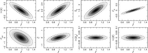
We find that the constraints generated from the reduced bispectrum contain no strong degeneracies between f and the radiative transfer parameters (see Fig. 3). The reduced bispectrum does however exhibit some degeneracies between f, and the galaxy bias parameters, |$\tilde{b}_{1}$| and |$\tilde{b}_{2}$|.
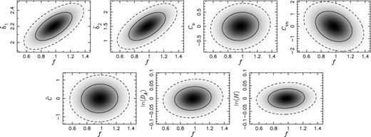
Two-dimensional joint marginalized likelihood distributions computed from the fiducial LAE galaxy reduced bispectrum alone (no Lyα radiative transfer effects, but including marginalization over Cv, Cvv and |$\tilde{C}$|). We show the correlations between the growth rate of structure, f, and various parameters including (clockwise from top left): the linear bias, |$\tilde{b}_{1}$|, non-linear bias, |$\tilde{b}_{2}$|, linear peculiar velocity Lyα effect, Cv, non-linear peculiar velocity Lyα effect, Cvv, the non-linear combination of other radiative transfer effect, |$\tilde{C}$|, angular diameter distance, ln (DA), and the Hubble rate ln (H). The solid and dashed curves show the 1σ and 2σ joint marginalized constraints, respectively.
Equations (51)–(53) show that the reduced bispectrum determines the following parameter combinations:
|$\tilde{b}_1$| from the overall amplitude of the first four terms in |$\hat{K}_2^{(s)}$|,
|$\tilde{b}_2/\tilde{b}_1$| from a constant, k-independent term in |$\hat{K}_2^{(s)}$|,
|$\tilde{\beta }(1-C_v)$| from |$\hat{K}_1^{(s)}$| and the term proportional to G(s)2 in |$\hat{K}_2^{(s)}$|,
|$\tilde{\beta }\tilde{C}$| from the second term in |$\hat{K}_2^{(s)}$| and
|$\tilde{\beta }$| from the last term before |${\cal O}(\mu ^4)$| in |$\hat{K}_2^{(s)}$|.
Recalling |$\tilde{\beta }=f/\tilde{b}_1$|, there are five unknown variables (|$\tilde{b}_1$|, |$\tilde{b}_2$|, f, |$\tilde{C}_v$| and |$\tilde{C}$|), and the reduced bispectrum yields five combinations of these variables.
From the Fisher matrix calculations, we find that the reduced bispectrum primarily yields |$\tilde{b}_2/\tilde{b}_1$| and |$\tilde{\beta }$|. The information on |$\tilde{b}_1$| coming from the first four terms in |$\hat{K}_2^{(s)}$| breaks a complete degeneracy between |$\tilde{b}_2$| and |$\tilde{b}_1$| and f, but correlations between these parameters still remain. One can see this in the first two panels in Fig. 3. On the other hand, we do not find much correlation between f and the radiative transfer parameters, |$\tilde{C}$|, |$\tilde{C}_v$| and |$\tilde{C}_{vv}$| (see the third to fifth panels of Fig. 3).
While the reduced bispectrum does break the degeneracy between f and Cv seen in our power spectrum analysis, it cannot provide a strong constraint on f. In the fourth column of Table 4, we provide the 1σ constraints generated from the one-dimensional likelihood distribution for f. In the fiducial case with no additional priors, we find the 1σ constraint on the growth rate of structure, f, to be 0.16 (17 per cent). It is important to note that, while the constraints are relatively weak, they are on f as opposed to |$\tilde{\beta }$|. Also, |$\tilde{\beta }$| and Cv are totally degenerate in the LAE power spectrum, and thus the error bar on |$\tilde{\beta }$| is infinite unless we put a prior on Cv. Therefore, the reduced bispectrum provides a massive improvement on the constraint on f: the error bar shrinks from infinity to 17 per cent.
We show the 1σ constraints expected from the reduced bispectrum (RBS), the power spectrum combined with the bispectrum (PS+BS) and the power spectrum combined with the reduced bispectrum (PS+RBS). No Lyα radiative transfer effects are included, but the likelihood is marginalized over Cv, Cvv and |$\tilde{C}$|. The first five rows show the 1σ constraints on f for various priors on Cv, after marginalizing over |$\tilde{b}_{1}$|, |$\tilde{b}_{2}$|, |$\tilde{C}$|, Cv, Cvv, ln (DA), ln (H) and the amplitude [ln (A)]. The last six rows show the 1σ constraints on the distance parameters, ln (DA) and ln (H), marginalized over the remaining model parameters.
| Priors on Cv | Parameter | Model | RBS | PS+BS | PS+RBS |
|---|---|---|---|---|---|
| 1σ (per cent) | 1σ (per cent) | 1σ (per cent) | |||
| No priors | f | Fiducial | 0.1645 (16.92) | 0.1602 (16.48) | 0.1579 (16.24) |
| Perfect knowledge | f | Fiducial | 0.1635 (16.82) | 0.0507 (5.21) | 0.0565 (5.81) |
| 0.01 | f | Fiducial | 0.1635 (16.82) | 0.0520 (5.35) | 0.0576 (5.93) |
| 0.1 | f | Fiducial | 0.1636 (16.83) | 0.1055 (10.85) | 0.1063 (10.93) |
| 0.5 | f | Fiducial | 0.1642 (16.89) | 0.1555 (16.00) | 0.1535 (15.79) |
| No priors | ln (DA) | Fiducial | 0.0303 (3.03) | 0.0076 (0.76) | 0.0103 (1.03) |
| 0.01 | ln (DA) | Fiducial | 0.0301 (3.01) | 0.0075 (0.75) | 0.0101 (1.01) |
| 0.1 | ln (DA) | Fiducial | 0.0302 (3.02) | 0.0075 (0.75) | 0.0102 (1.02) |
| No priors | ln (H) | Fiducial | 0.0251 (2.51) | 0.0084 (0.84) | 0.0115 (1.15) |
| 0.01 | ln (H) | Fiducial | 0.0249 (2.49) | 0.0083 (0.83) | 0.0112 (1.12) |
| 0.1 | ln (H) | Fiducial | 0.0249 (2.49) | 0.0083 (0.83) | 0.0113 (1.13) |
In the left-hand panel of Fig. 4, we show the one-dimensional likelihood distributions for the growth rate of structure, f, for various priors on Cv. The addition of priors to Cv does not improve the constraints on f from the reduced bispectrum alone, as the reduced bispectrum contains no degeneracy between f and Cv.
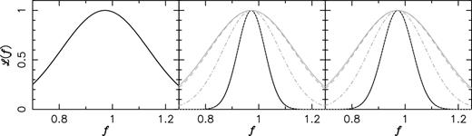
One-dimensional marginalized likelihood distributions for the growth rate of structure, f, for the fiducial case (no Lyα radiative effects added, but including marginalization over Cv, Cvv and |$\tilde{C}$|) generated from (left) the LAE galaxy reduced bispectrum only, (centre) the LAE galaxy power spectrum combined with the LAE galaxy bispectrum and ( right) the LAE galaxy power spectrum combined with the LAE galaxy reduced bispectrum. The various curves denote different priors added to Cv; black solid: perfect knowledge of Cv, grey dotted: |$\sigma _{C_{v}} = 0.01$|, grey dot–dashed: |$\sigma _{C_{v}} = 0.1$|, grey dashed: |$\sigma _{C_{v}} = 0.5$| and grey solid: no priors added.
In the fourth column of Table 4, we also provide the 1σ constraints from the one-dimensional likelihoods for ln (DA) and ln (H) given various priors on Cv. We find that (independent of priors on Cv) the fiducial LAE galaxy reduced bispectrum can recover the angular diameter distance scale at 3 per cent and the Hubble rate at 2.5 per cent. This should be contrasted with the 1.1 and 1.3 per cent errors on DA and H expected from the fiducial LAE galaxy power spectrum. Clearly, the reduced bispectrum alone provides weaker distance constraints. This is not surprising, as the distance information is contained in the shape of the power spectrum [e.g. baryon acoustic oscillation (BAO) and Alcock–Paczynski (AP) test], which is largely divided out in the reduced bispectrum.
5.2 LAE reduced bispectrum
We now consider the inclusion of Lyα radiative transfer effects by adding the linear Lyα radiative transfer model parameters, CΓ = 0.05, Cρ = −0.39 and Cv = 0.11 from Wyithe & Dijkstra (2011). The inclusion of these parameters modifies the effective bias parameters, |$\tilde{b}_{1}$| and |$\tilde{b}_{2}$|, and the Lyα radiative transfer effects associated with |$\tilde{C}$|. We still set the fiducial values of the second-order Lyα radiative transfer coefficients to vanish. Although we set Cvv = 0, we still marginalize over Cvv in our models.
In the fourth column of Table 5, the 1σ constraints on f, ln (DA) and ln (H) are generated from the likelihood distributions for various priors on Cv as per the previous section. With the inclusion of the Lyα effects, the precision with which we can constrain the growth rate of structure f has been reduced to an error of 0.21 (22 per cent) compared to 0.16 (17 per cent) for the fiducial model. Once again, this is due to the reduced effective linear galaxy bias, which reduces the signal-to-noise ratio of the LAE power spectrum relative to the shot noise.
Same as Table 4, but for the first-order Lyα radiative transfer effects given by CΓ = 0.05, Cρ = −0.39 and Cv = 0.11.
| Priors on Cv | Parameter | Model | RBS | PS+BS | PS+RBS |
|---|---|---|---|---|---|
| 1σ (per cent) | 1σ (per cent) | 1σ (per cent) | |||
| No priors | f | LAE effects included | 0.2104 (21.64) | 0.2039 (20.97) | 0.2014 (20.72) |
| Perfect knowledge | f | LAE effects included | 0.2089 (21.49) | 0.0632 (6.50) | 0.0672 (6.91) |
| 0.01 | f | LAE effects included | 0.2089 (21.49) | 0.0645 (6.64) | 0.0685 (7.05) |
| 0.1 | f | LAE effects included | 0.2090 (21.50) | 0.1262 (12.98) | 0.1270 (13.06) |
| 0.5 | f | LAE effects included | 0.2099 (21.59) | 0.1965 (20.21) | 0.1943 (19.99) |
| No priors | ln (DA) | LAE effects included | 0.0378 (3.78) | 0.0099 (0.99) | 0.0120 (1.20) |
| 0.01 | ln (DA) | LAE effects included | 0.0376 (3.76) | 0.0098 (0.98) | 0.0119 (1.19) |
| 0.1 | ln (DA) | LAE effects included | 0.0376 (3.76) | 0.0099 (0.99) | 0.0119 (1.19) |
| No priors | ln (H) | LAE effects included | 0.0305 (3.05) | 0.0107 (1.07) | 0.0133 (1.33) |
| 0.01 | ln (H) | LAE effects included | 0.0302 (3.02) | 0.0106 (1.06) | 0.0131 (1.31) |
| 0.1 | ln (H) | LAE effects included | 0.0303 (3.03) | 0.0107 (1.07) | 0.0132 (1.32) |
6 COSMOLOGICAL CONSTRAINTS FROM COMBINING THE POWER SPECTRUM AND BISPECTRUM
We next discuss the improvements on the cosmological constraints available when we combine the LAE power spectrum with either the LAE reduced bispectrum or the bispectrum. When combining the reduced bispectrum (and the bispectrum) to the information from the power spectrum, we assume that there is no covariance between the power spectrum and the reduced bispectrum (or the bispectrum), which is incorrect. Therefore, the numerical values of the 1σ constraints on various parameters reported here should be considered as lower bounds.
6.1 Fiducial LAE model for the power spectrum and bispectrum
We first consider our fiducial model in which all Lyα radiative transfer coefficients are set to zero. The number of parameters in this model is nine. While the LAE galaxy reduced bispectrum is insensitive to the amplitude of the matter power spectrum, we must marginalize over the amplitude information in the LAE galaxy power spectrum. The parameters include four cosmological parameters: the amplitude [ln (A)], f, ln (DA) and ln (H); three radiative transfer parameters: Cv, Cvv and |$\tilde{C}$|; and the linear and non-linear galaxy biases: |$\tilde{b}_{1}$| and |$\tilde{b}_{2}$|.
6.1.1 Combined power spectrum and reduced bispectrum
Fig. 5 shows the expected constraints from a joint analysis of the reduced bispectrum and the power spectrum on various pairs of parameters involving f. Comparing this figure with Fig. 3, we find that adding the power spectrum does not improve the constraints on f and the bias parameters very much, but improves the constraints on all the other parameters. Fig. 6 shows this more clearly: adding the power spectrum information does not improve the constraint on f, but it substantially improves the constraint on Cv.
Two-dimensional joint marginalized likelihood distributions computed from the fiducial LAE galaxy power spectrum combined with the fiducial LAE galaxy reduced bispectrum (no Lyα radiative transfer effects added, but including marginalization over Cv, Cvv and |$\tilde{C}$|). We show the correlations between the growth rate of structure, f, and various parameters including (clockwise from top left): the amplitude, ln (A), linear bias, |$\tilde{b}_{1}$|, non-linear bias, |$\tilde{b}_{2}$|, linear peculiar velocity Lyα effect, Cv, non-linear peculiar velocity Lyα effect, Cvv, the non-linear combination of other radiative transfer effect, |$\tilde{C}$|, angular diameter distance, ln (DA), and the Hubble rate, ln (H). The solid and dashed curves show the 1σ and 2σ joint marginalized constraints, respectively.
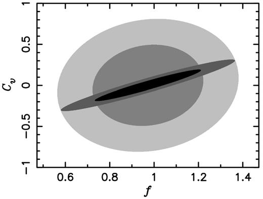
Comparison of the joint two-dimensional constraints on f and Cv. Outer two ellipses correspond to the 1σ and 2σ constraints generated from the fiducial LAE galaxy reduced bispectrum only. Two narrower ellipses correspond to the 1σ and 2σ constraints generated from the fiducial LAE galaxy power spectrum combined with the fiducial LAE galaxy reduced bispectrum.
What does this imply? This implies that the uncertainty in f is now dominated by the correlation between f and the bias parameters – the correlation that we have discussed in Section 5.1. Comparing the fourth and sixth columns of Table 4 shows this quantitatively.
Comparing the fourth and sixth columns of Table 4 also shows that adding the power spectrum does improve the constraints on DA and H substantially, as the power spectrum contains features such as BAO and AP test, whereas such information is largely cancelled out in the reduced bispectrum.
Nevertheless, as the reduced bispectrum still has some sensitivity to these features (i.e. cancellation is not exact), the constraints on DA and H from the power spectrum and the reduced bispectrum are slightly better than those from the power spectrum alone. Comparing the third column of Table 2 and the sixth column of Table 4, we find that the expected constraints improve from 1.1 to 1.0 per cent for DA and 1.3 to 1.2 per cent for H.
6.1.2 Combined power spectrum and bispectrum
Next, we combine the power spectrum with the bispectrum (rather than the reduced bispectrum). As far as f is concerned, we have the same story: adding the power spectrum does not improve the expected error bar on f (see the fifth column of Table 4).
On the other hand, a joint analysis of the power spectrum and the bispectrum yields a significant improvement on the angular diameter distance and the Hubble rate. This is because the bispectrum also contains the BAO features and the AP test in its wavenumber dependence. However, this could be due to our ignoring a covariance between the power spectrum and the bispectrum: a correlation between them would degrade the constraints in a joint analysis. This point requires a further investigation.
6.2 LAE model for power spectrum combined with bispectrum
Finally, we consider the inclusion of Lyα radiative transfer effects on the recovery on f, ln (DA) and ln (H), by adding the linear Lyα radiative transfer parameters, CΓ = 0.05, Cρ = −0.39 and Cv = 0.11 from Wyithe & Dijkstra (2011). Table 5 shows the results: the expected constraints are slightly weaker than those from the fiducial case, which is again due to a smaller effective bias, |$\tilde{b}_1$|, reducing the amplitude of the signal relative to the shot noise.
7 SUMMARY AND CONCLUSION
In this paper, we have studied how the radiative transfer effects alter the power spectrum and bispectrum of LAE galaxies, and how we can use these properties to separate the radiative transfer effects and the cosmological effects, so that we can improve the cosmological constraints derived from them.
First, as a follow-up to Wyithe & Dijkstra (2011), we show that the growth rate of structure (f ) and the parameter Cv describing the radiative transfer effects of velocity gradients are completely degenerate in the linear power spectrum. Next, by performing a perturbation theory expansion of the Lyα radiative transfer effects, we derive the next-to-leading-order corrections to the density fields of LAE galaxies. This allows us to derive the leading-order expression for the bispectrum of LAE galaxies. We then show that the reduced bispectrum alone can determine f and Cv separately, leaving no degeneracy between them. Adding the power spectrum information to the reduced bispectrum does not improve the precision of f further, as the precision of f is now limited by remaining correlations between f and the galaxy bias parameters, b1 and b2.
We find that HETDEX-like surveys of LAE galaxies can determine f to about 20 per cent accuracy, if we do not assume any prior information on Cv. Including the prior on Cv, the uncertainty on f can be reduced down to 7 per cent. Note that this is the uncertainty on f, rather than on β = f/b1.
We find that the constraints on the angular diameter distance and the Hubble expansion rate are not directly affected by the radiative transfer parameters (with the caveat that we have assumed that the effect of the UV ionizing background fluctuation is not scale dependent). The only indirect effect is a slight reduction of the effective linear galaxy bias, which reduces the amplitude of the LAE power spectrum with respect to the shot noise, thus slightly increasing the uncertainties in the angular diameter distance and the Hubble rate. Comparison between the top and bottom panels of Fig. 7 shows this graphically.
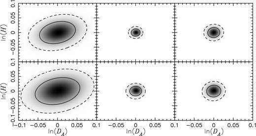
Two-dimensional joint marginalized likelihood distributions for the angular diameter distance, DA, and the Hubble rate, H. Shown also are the 1σ (solid) and 2σ (dashed) joint likelihood contours. From left to right shown are the constraints generated from the LAE galaxy reduced bispectrum only, the LAE galaxy power spectrum and bispectrum combined, and the LAE galaxy power spectrum and reduced bispectrum combined. Top panels: fiducial case, with no Lyα radiative transfer effects added to the fiducial parameters, but marginalizing over Cv, Cvv and |$\tilde{C}$|. Bottom panels: the inclusion of the first-order Lyα radiative transfer effects, Cv = 0.11, CΓ = 0.05 and Cρ = −0.39, and marginalizing over Cv, Cvv and |$\tilde{C}$|.
Finally, to summarize the results of this work, we provide Table 6 detailing the constraints on β, f, DA and H expected from HETDEX-like surveys. This table shows how powerful such surveys are in terms of measuring the distance, the expansion rate, as well as the growth rate of the structure in a high-redshift universe, and the determination of these quantities is not significantly compromised by the Lyα radiative transfer effect.
Summary of the relevant 1σ constraints (and fractional errors) generated from the one-dimensional likelihood distributions for β, f, ln (DA) and ln (H). Models considered are ‘Galaxy’ (no Lyα radiative transfer effects, and no marginalization over the radiative transfer parameters), ‘Fiducial’ (no Lyα radiative transfer effects, but marginalized over the radiative transfer parameters) and ‘LAE effects’ (non-zero Lyα radiative transfer parameters are included and marginalized over). We consider a power spectrum only model (PS), reduced bispectrum only (RBS), power spectrum combined with the bispectrum (PS+BS) and the power spectrum combined with the reduced bispectrum (PS+RBS). We explore three priors on the Lyα radiative parameter associated with the peculiar velocity, Cv: no prior at all, prior of 0.01 and prior of 0.1.
| Priors on Cv | Parameter | Model | PS | RBS | PS+BS | PS+RBS | ||||
|---|---|---|---|---|---|---|---|---|---|---|
| 1σ | per cent | 1σ | per cent | 1σ | per cent | 1σ | per cent | |||
| No priors | β | Galaxy | 0.0213 | 4.8 | – | – | – | – | – | – |
| No priors | f | Fiducial | – | – | 0.1645 | 16.9 | 0.1602 | 16.5 | 0.1579 | 16.2 |
| 0.01 | f | Fiducial | 0.0218 (|$\tilde{\beta }$|) | 4.9 | 0.1635 | 16.8 | 0.0520 | 5.3 | 0.0576 | 5.9 |
| 0.1 | f | Fiducial | 0.0491 (|$\tilde{\beta }$|) | 11.1 | 0.1636 | 16.8 | 0.1055 | 10.9 | 0.1063 | 10.9 |
| No priors | f | LAE effects | – | – | 0.2104 | 21.6 | 0.2039 | 21.0 | 0.2014 | 20.7 |
| 0.01 | f | LAE effects | 0.0283 (|$\tilde{\beta }$|) | 5.6 | 0.2089 | 21.5 | 0.0645 | 6.7 | 0.0685 | 7.1 |
| 0.1 | f | LAE effects | 0.0633 (|$\tilde{\beta }$|) | 12.5 | 0.2090 | 21.5 | 0.1262 | 13.0 | 0.1270 | 13.1 |
| No priors | ln (DA) | Fiducial | 0.0110 | 1.10 | 0.0303 | 3.03 | 0.0076 | 0.76 | 0.0103 | 1.03 |
| No priors | ln (DA) | LAE effects | 0.0128 | 1.28 | 0.0378 | 3.78 | 0.0099 | 0.99 | 0.0120 | 1.20 |
| No priors | ln (H) | Fiducial | 0.0132 | 1.32 | 0.0251 | 2.51 | 0.0084 | 0.84 | 0.0115 | 1.15 |
| No priors | ln (H) | LAE effects | 0.0151 | 1.51 | 0.0305 | 3.05 | 0.0107 | 1.07 | 0.0133 | 1.33 |
ACKNOWLEDGMENTS
BG acknowledges the support of the Australian Postgraduate Award. The Centre for All-sky Astrophysics is an Australian Research Council Centre of Excellence, funded by grant CE110001020. BG would also like to acknowledge the partial travel support to the USA provided by the Astronomical Society of Australia (ASA). BG would like to thank the Texas Cosmology Center at the University of Texas at Austin for their hospitality during this work, and the Kavli Institute for the Physics and Mathematics of the Universe for their hospitality during the completion of this work. We would like to thank Donghui Jeong for helpful discussions contributing to the completion of this work as well as to the derivation provided in Appendix C, and Eric Gawiser for useful comments on the draft. EK is supported in part by NSF grant AST-0807649 and NASA grant NNX08AL43G.
In equation (12), we do not consider the scale dependence of the ionizing background fluctuations, which is the major difference between our expression and the expression in Wyithe & Dijkstra (2011). The ionizing background fluctuations are expected to be scale dependent, important on large scales (set by the mean free path of the ionizing photons) and becoming negligible on small scales. However, including the scale dependence associated with the ionizing background fluctuations increases the model complexity, providing additional model degeneracies. We feel that this simplification is justified since the transmission models investigated by Wyithe & Dijkstra (2011) find the magnitude of ionizing background fluctuations (CΓ) to be small compared to the other two radiative transfer effects. Hence, while ignoring the scale dependence is a simplification, the overall impact of removing this scale dependence should be minor.
Throughout this work, we define the ‘perfect knowledge of Cv’ as a prior set to |$\sigma _{C_{v}} = 0.0001$|, which is to ensure that our Fisher matrix elements remain finite, yet still mimic the behaviour for perfectly understood parameters.
REFERENCES
APPENDIX A: Lyα RADIATIVE TRANSFER COEFFICIENTS
Throughout this work, we denote the Lyα radiative transfer effects as constants, which encompass the derivatives of the transmission function with respect to the Lyα radiative transfer effect. Here we outline the derivations for the first-order Lyα radiative transfer coefficients, from which the second-order constants can be easily calculated. In the following derivations, each of the Lyα radiative transfer effects is expressed as a function of an arbitrary transmission function, |$\mathcal {T}$| (Wyithe & Dijkstra 2011).
APPENDIX B: Lyα RADIATIVE TRANSFER KERNELS
Here we outline the derivation of the higher order real- and redshift-space kernels for the fluctuations in the number density of LAEs.
B1 Real-space Lyα kernels
B2 Redshift-space Lyα kernels
APPENDIX C: CALCULATION OF VB
APPENDIX D: DERIVATION OF THE BISPECTRUM DISTANCE DERIVATivES
To calculate the Fisher matrix for the angular diameter distance and the Hubble rate, we need to calculate derivatives of the bispectrum with respect to the distances, namely |$\frac{\mathrm{\partial} B(k_{1},k_{2},k_{3},\mu _{1},\mu _{2},\mu _{3})}{\mathrm{\partial} {\rm ln}(D_{{\rm A}})}$| and |$\frac{\mathrm{\partial} B(k_{1},k_{2},k_{3},\mu _{1},\mu _{2},\mu _{3})}{\mathrm{\partial} {\rm ln}(H)}$|. However, we are dealing with the variables k1, k2, k3, μ1, μ2 and μ3, which are not all independent of one another. Hence, we perform the chain rule with respect to the independent functions, k1, k2, k3(θ12, μ1, φ), μ1, μ2(μ1, φ) and μ3(k1, k2, θ12, μ1, φ). Here, we have written the dependent variables, k3, μ2 and μ3, as functions of the independent variables k1, k2, θ12, μ1 and φ, which fully describe the shape and orientation of the bispectrum triangles.
