


Abstract
GRB 130925A was an unusual gamma ray burst (GRB), consisting of three distinct episodes of high-energy emission spanning ∼20 ks, making it a member of the proposed category of ‘ultralong’ bursts. It was also unusual in that its late-time X-ray emission observed by Swift was very soft, and showed a strong hard-to-soft spectral evolution with time. This evolution, rarely seen in GRB afterglows, can be well modelled as the dust-scattered echo of the prompt emission, with stringent limits on the contribution from the normal afterglow (i.e. external shock) emission. We consider and reject the possibility that GRB 130925A was some form of tidal disruption event, and instead show that if the circumburst density around GRB 130925A is low, the long duration of the burst and faint external shock emission are naturally explained. Indeed, we suggest that the ultralong GRBs as a class can be explained as those with low circumburst densities, such that the deceleration time (at which point the material ejected from the nascent black hole is decelerated by the circumburst medium) is ∼20 ks, as opposed to a few hundred seconds for the normal long GRBs. The increased deceleration radius means that more of the ejected shells can interact before reaching the external shock, naturally explaining both the increased duration of GRB 130925A, the duration of its prompt pulses, and the fainter-than-normal afterglow.
INTRODUCTION
Gamma ray bursts (GRBs), discovered by Klebesadel, Strong & Olson (1973), are the most powerful explosions in the Universe. Mazets et al. (1981) and Kouveliotou et al. (1993) showed that GRBs can be divided into two classes based on their duration: long and short GRBs. These objects have different progenitors, with the short (≲2 s) GRBs believed to be the mergers of binary neutron-star systems and long GRBs arising from the collapse of a massive star (see Zhang et al. 2009 for a detailed discussion of GRB progenitors and classification). In both cases, it is generally believed that the prompt emission arises due to interactions within the outflow of material (see, e.g. Zhang 2007). Recently, Gendre et al. (2013), Stratta et al. (2013) and Levan et al. (2014) have proposed an additional category of ‘ultralong’ bursts, GRBs with durations of kiloseconds. These authors consider tidal disruption of a white-dwarf star by a massive black hole, and a GRB with a blue supergiant progenitor (larger than those of normal long GRBs) as possible causes of these ultralong bursts, with the latter being favoured. In contrast, Virgili et al. (2013) suggest that the ultralong GRBs simply represent the tail of the distribution of long GRBs.
With the exception of GRB 101225A, the ultralong GRBs show an X-ray afterglow, once the prompt emission is over. Such a feature is seen after most long GRBs, and is generally believed to occur when the material ejected by the GRB, which is travelling close to the speed of light, is decelerated by the circumburst medium (CBM). A shock forms and propagates into the medium, radiating by the synchrotron mechanism as it does so. This model is not uniformly accepted, with some authors (e.g. Genet, Daigne & Mochkovitch 2007; Uhm & Beloborodov 2007; Leventis, Wijers & van der Horst 2013) arguing that the late-time emission is strongly affected by emission from a reverse shock, which propagates back into the outflowing material once it is decelerated.
Regardless of their physical origin, GRB X-ray afterglows show a range of different light-curve behaviours (Evans et al. 2009), perhaps the most curious of which is the so-called ‘plateau’ phase (Nousek et al. 2006; Zhang et al. 2006) – a period during which the afterglow fades slowly, if at all. The most widely accepted explanation for this plateau is that there is an ongoing injection of energy into the shocked CBM (e.g. Liang, Zhang & Zhang 2007). Such plateaux are not seen in all afterglows; Evans et al. (2009) found them in <70 per cent of bursts. In contrast to the light curves, the spectra of X-ray afterglows show little variation, with the photon index (Γ; N(E)dE∝E− Γ) distribution1 being approximately Gaussian, with a mean of 2.0 and a full width at half-maximum (FWHM) of 0.7 (Evans et al. 2009, the live XRT GRB catalogue2). This spectrum is generally found not to evolve with time (e.g. Butler & Kocevski 2007; Shen et al. 2009).
In this paper, we consider GRB 130925A, a GRB which triggered Swift, Fermi, Konus-Wind, INTEGRAL and MAXI, and had a duration of >5 ks, making it a candidate ultralong GRB. However, this burst is also unusual in that its late-time X-ray data showed a strong hard-to-soft spectral evolution with time. Recently, Bellm et al. (2014) have analysed Swift, Chandra and NuSTAR data of this burst, and claim the presence of multiple afterglow components; however, we shall show that a simpler emission model can explain the data presented here.
Throughout this paper, we assume a cosmology with H0 = 71 km s−1 Mpc−1, Ωm = 0.27, Ωvac = 0.73, and we made use of the online Cosmology Calculator3 (Wright 2006). Errors are at the 90 per cent level unless otherwise stated.
OBSERVATIONS
GRB 130925A triggered the INTEGRAL SPI-ACS instrument at 04:09:25 ut on 2013 September 25 (Savchenko et al. 2013); hereafter, this time is referred to as T0. Fermi-GBM triggered just after this at 04:09:26.73 ut (Fitzpatrick 2013; Jenke 2013), and Swift-BAT triggered at 04:11:24 ut (Lien et al. 2013); the GRB was also detected by Konus-Wind in waiting mode (Golenetskii et al. 2013). These triggers all correspond to the same episode of emission, which lasted around 900 s (in the 15–350 keV BAT data the total duration above the background level was 846 s, while T90 = 179 s). There was an earlier ‘precursor’ lasting 6 s which triggered the Fermi-GBM at 03:56:23.29 ut (T0 − 781 s), this was also seen by Konus-Wind but not by INTEGRAL or BAT. The Fermi trigger also resulted in an automated slew of the satellite to orient the LAT boresight towards the GRB (Jenke 2013); however, no emission was detected in the 0.1–10 GeV band, with an upper limit (95 per cent confidence) of 4.8 × 10⁻¹⁰ erg cm−2 s−1 (Kocevski et al. 2013).
The Swift-XRT began observing 147.4 s after the BAT trigger and found a bright, uncatalogued X-ray source (Lien et al. 2013).
A second episode of high-energy emission occurred at T0 + 2000–3000 s and was seen by both Konus-Wind and INTEGRAL; the GRB was not observable by Swift or Fermi at this time due to Earth occultation. At 05:13:41 (T0 + 3.8 ks), the MAXI Gas Slit Camera also triggered on the GRB (Suzuki et al. 2013) which still had a flux of 290 mCrab: this corresponds to the time of a third interval of high-energy emission detected by Konus-Wind, INTEGRAL and Fermi-GBM (the object was outside the Swift-BAT field of view). As with the initial episode, Fermi-LAT did not detect anything, with an upper limit of 1.6 × 10⁻⁹ erg cm−2 s−1 (0.1–10 GeV; Kocevski et al. 2013). At T0 + 4.8 ks Swift observations resumed, and the XRT detected a flare which was also seen by the BAT, INTEGRAL and GBM although at much lower levels than from the three main emission episodes. Two further flares were detected by XRT on the subsequent spacecraft orbits,4 before the X-ray light curve settled down to the decay ubiquitous to X-ray GRB afterglows. Fig. 1 shows the multi-observatory light curve of the prompt emission and flaring episodes. For each instrument, we obtained a single counts-to-flux conversion factor using the joint spectral fit to the first emission episode (Section 3) and multiplied the count rate by this value. This neglects the effects of spectral evolution (which are, however, incorporated in the modelling in Section 3) but shows the relative strength of the various pulses in different energy bands. The full XRT light curve [taken from the XRT light-curve repository5 (Evans et al. 2007, 2009) on 2014 March 17] is given in Fig. 2.
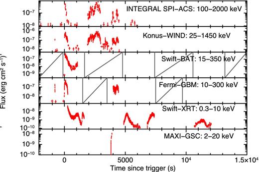
Multi-observatory light curves of the prompt and flaring emission. These were built assuming a constant-spectral model, as fitted to the Episode 1 data (Section 3). The fluxes are given in each instrument's native band, and in the observer frame. This reveals the relative flux at different energies, for each pulse, illustrating the spectral variation from pulse to pulse. The data have been binned to a minimum signal-to-noise ratio per bin of 5, using the approach of Evans et al. (2010). As Swift and Fermi are in low-Earth orbits, the times when the source was outside of their field of view are marked by the grey diagonal lines. For Swift-XRT, whenever the source was in the field of view, it was detected; so to keep the plot simple, we do not mark the times when it was not in the field (although these will be similar to the BAT times). Similarly for MAXI which could only observe the GRB for ∼2 min of each ∼93 min orbit (and only detected the GRB in one orbit), we do not include the observability intervals.
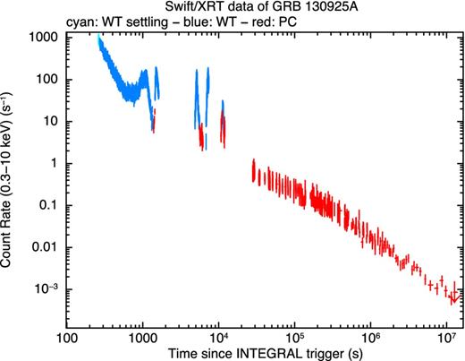
The full 0.3–10 keV X-ray light curve, from the XRT light-curve repository (Evans et al. 2009).
At longer wavelengths, an infrared counterpart was detected by GROND (Greiner et al. 2008) in observations starting at T0 + 567 s (Sudilovsky, Kann & Greiner 2013), and by RATIR (Butler et al. 2012) in observations starting at T0 + 8.28 ks (Butler et al. 2013). VLT spectroscopy found the GRB redshift to be 0.347 (Vreeswijk et al. 2013) in agreement with our own observations (Section 2.1). The Swift-UVOT did not detect the burst; however, the IR colours from Sudilovsky et al. (2013) suggest that there is significant dust in the line of sight, consistent with the lack of UVOT detection. Radio observations at 230 GHz beginning 1.1 d after the trigger found no source, with a 3σ upper limit of 1.89 mJy (Zauderer, Berger & Petitpas 2013), and observations at 93 GHz beginning 1.2 d after the trigger also found no source, with a 3σ upper limit of 0.6 mJy. Later, radio observations taken with ATCA between ∼15 and 21 d after the trigger detected emission at the GRB location, with fluxes of ∼140–190 μJy at frequencies between 5.5 and 19 GHz (Bannister et al. 2013)
Observations with the HubbleSpace Telescope (HST) revealed the host galaxy to be a nearly edge-on spiral, but with signs of disturbance, with the bulge being elongated perpendicular to the disc, suggesting that the host is a polar ring galaxy. The afterglow was located in the HST images to be 0.12 arcsec offset from the centre of the galaxy, which is ∼600 pc in projection (Tanvir et al. 2013). HST observed the object again at two further epochs ( Tanvir et al., in preparation).
GTC imaging and spectroscopic observations of the GRB 130925A host galaxy
Imaging of the host galaxy of GRB 130925A in the griz bands was carried out with the 10.4 m Gran Telescopio Canarias (GTC) telescope equipped with the OSIRIS instrument on the nights of 2013 Nov 4–5. The images were acquired in 2 × 2 binning, providing a pixel scale of 0.25 arcsec pix−1. Photometric calibration was performed by observation of standard star SA114−656 (Smith et al. 2002). The images were dark-subtracted and flat-fielded using custom iraf6 routines. Aperture photometry was done using daophot tasks implemented in iraf. Table 1 displays the host galaxy AB magnitudes. The g-band magnitude was used to scale the flux of the host galaxy GTC spectrum (see Table 2).
Observing log of the host galaxy imaging. The magnitudes are in the AB system with no reddening correction. The r-band measurement is based on data taken in two consecutive nights. Errors are at the 1σ level.
| Observing date | Exposure | Filter | Magnitude |
|---|---|---|---|
| (Start–End) 2013 ut | time (s) | (AB) | |
| Nov 5.111541–5.116603 | 3 × 120 | g | 22.72 ± 0.08 |
| Nov 4.083744–5.130114 | 4 × 90 + 3 × 60 | r | 21.94 ± 0.05 |
| Nov 5.117194–5.120173 | 3 × 60 | i | 21.68 ± 0.07 |
| Nov 5.120764–5.126661 | 5 × 75 | z | 21.16 ± 0.07 |
Emission lines identified in the host galaxy of GRB 130925A, revealing the redshift to be ∼0.348. Errors are at the 1σ level.
| Ion | λobs | λrest | z | FWHM | Observed flux |
| (Å air) | (Å air) | (Å) | (erg cm−2 s−1) | ||
| [O ii] | 5028.5 ± 0.1 | 3728.815 | 0.34855 | 9.7 ± 0.5 | (1.68 ± 0.09) × 10−16 |
| Hβ | 6555.8 ± 0.3 | 4861.363 | 0.34855 | 9.7 ± 0.5 | (7.1 ± 0.4) × 10−17 |
| |${\rm [O\,\small {III}]}$| | 6685.8 ± 0.5 | 4958.911 | 0.34824 | 10.2 ± 0.4 | (3.9 ± 0.1) × 10−17 |
| |${\rm [O\,\small {III}]}$| | 6750.5 ± 0.2 | 5006.843 | 0.34825 | 10.2 ± 0.4 | (1.16 ± 0.04) × 10−16 |
A simple single stellar population fit to the integrated host magnitudes using Bruzual & Charlot (1993) models, a Calzetti et al. (2000) extinction curve and redshift of z = 0.348, gives acceptable fits for a young stellar population (∼30 Myr) and substantial extinction (AV ∼ 2.2 mag). However, we caution that the morphology of the host (Tanvir et al. 2013), in particular the presence of a red bulge and blue disc (Tanvir et al. in preparation), indicates that more complex models may be required to characterize the host properties.
In addition, spectral observations were carried out with the GTC(+OSIRIS) on 2013 Nov 5, between 01:26 ut and 02:22 ut, with a total exposure time of 3 × 900 s. The spectra were acquired with grism R1000B, providing a spectral range of 3615–7760 Å. The data were taken with a slit width of 1.49 arcsec, resulting in a resolution of R ∼ 550 (estimated using weak sky lines). Data reduction followed standard procedures using custom routines under iraf and python. The spectra were bias-corrected and flat-fielded. We have chosen a wavelength solution based on calibration arcs taken with a slit width of 1.2 arcsec to achieve better accuracy than the one we also obtained with the 1.49 arcsec one. The flux of the final spectra were calibrated with the spectrophotometric standard G191-B2B (Oke 1990) and scaled to the host galaxy g-band magnitude (see Table 1) to account for the slit losses. The spectrum is shown in Fig. 3. We identified several lines in the spectrum, at a common redshift of ∼0.348 (see Table 2) which we adopt as the redshift of the GRB hereafter; this gives a luminosity distance of 1.836 Gpc. We derive a lower limit on the star formation rate (SFR) from the strength of the [O ii] line, applying the calibration of Kennicutt (1998), SFR (M⊙ yr−1) = (1.4 ± 0.4) × 10−41|$L_{\rm [O\,\small {II}]}$|. Using the measured line luminosity as a lower limit implies SFR(M⊙ yr−1) > 0.95 M⊙ yr−1, a lower value than inferred from other GRB host galaxies (Christensen, Hjorth & Gorosabel 2004).
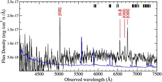
The optical spectrum of GRB 130925A from the GTC. The blue line shows the level of the errors. The tick marks at the top indicate the atmospheric sky lines/bands. Various emission lines can be seen in the spectrum at a redshift of 0.348.
PROMPT EMISSION AND FLARES
Due to the unusual duration of GRB 130925A, we examined whether the intervals of high-energy emission look like typical GRB prompt emission pulses (apart from their duration). Based on the light curve in Fig. 1, we defined four intervals of high-energy emission, and extracted spectra for each of these from whichever instruments were on target at the time, as shown in Table 3.7 For Fermi-GBM data, a spectrum was created individually for each detector which detected the source during the time interval.
Times of the prompt emission episodes, over which high-energy spectra were extracted, and the five X-ray flares for which Swift spectra were obtained. We also note which missions and instruments gathered spectroscopic data during each episode.
| Name | Timesa | Instruments |
|---|---|---|
| Precursor | −800 to −778 | Fermi-GBMb, Konus-Wind |
| Episode 1 | −5 to 300 | Fermi-GBMc, Konus-Wind, Swift-BAT |
| Episode 2 | 1800–3000 | Konus-Wind |
| Episode 3 | 3800–4500 | Fermi-GBMd, Konus-Wind |
| Flare 1 | 780–1200 | Swift-XRT and BAT |
| Flare 2 | 1200–1400 | Swift-XRT and BAT |
| Flare 3 | 4750–5350 | Swift-XRT and BAT |
| Flare 4 | 6680–7270 | Swift-XRT and BAT |
| Flare 5 | 10530–11590 | Swift-XRT |
aTimes in seconds since T0.
bData from four Na i detectors.
cData from one BGO detector and two Na i detectors.
dData from three Na i detectors.
We fitted the spectra of these time intervals in xspec (Arnaud 1996) with three models: a power law, cut-off power law and Band function (Band et al. 1993). For each fit, the parameters were tied to be the same for all instruments, but a multiplicative normalization factor was allowed to vary between them to allow for calibration differences in the absolute flux level. For the precursor, the cut-off power law and Band models offered no significant improvement over the simple power law. For the other spectra, the cut-off power law was significantly better than the simple power law. The Band function offered no further improvement, tending towards unconstrained highly negative values for the high-energy index, at which point the Band function behaves as a cut-off power law. The best-fitting spectral parameters for the cut-off power law and Band model fits are given in Table 4.
Details of the spectral fits to the episodes of prompt emission.
| Cut-off power law | Band function | |||||||
|---|---|---|---|---|---|---|---|---|
| Name | Fluence | Photon index | Epeak | χ2 (ν) | Γlow | Γhigh | Epeak (keV) | χ2 (ν) |
| (erg cm−2) | (Γ) | (keV) | (keV) | |||||
| (15–350 keV) | ||||||||
| Precursor | 6.8 × 10⁻⁷ | |$2.06^{+0.28}_{-0.21}$| | – | 604 (511)a | ||||
| Episode 1 | 8.0 × 10⁻⁵ | 1.91 ± 0.03 | |$65^{+13}_{-16}$| | 670 (436) | 1.91 ± 0.03 | >2.9 | |$65^{+13}_{-16}$| | 670 (435) |
| Episode 2 | 3.8 × 10⁻⁴ | |$1.55^{+0.04}_{-0.05}$| | |$175^{+13}_{-10}$| | 10−5 (0)b | ||||
| Episode 3 | 6.0 × 10⁻⁵ | |$1.58^{+0.12}_{-0.13}$| | |$94^{+14}_{-10}$| | 410 (363) | |$1.57^{+0.12}_{-0.13}$| | >2.9 | |$94^{+14}_{-11}$| | 410 (362) |
aThe precursor pulse was best fitted as a simple power law.
bThe Konus-Wind spectrum, which is the only one available for this episode, contains only three bins. Even so, the cut-off power law is very clearly a much better fit to the data (for the power-law fit, χ2 = 380.5 for ν = 1); however, it also has 0 degrees of freedom so a |$\chi _{\nu }^{2}$| value cannot be produced. We did not fit the Band model to this spectrum as it has −1 degrees of freedom.
We also created spectra covering the five flares that are seen in the XRT light curve (Table 3). For the first four spectra, we have both Windowed Timing (WT) mode XRT data and BAT data (taken in survey mode). Although the source was not detected by BAT during the second flare, the data provide constraints. The final flare was too faint for BAT to make a meaningful contribution, but we have both WT and Photon Counting (PC) mode data for that flare. Following the latest calibration guidance,8 as this source is moderately absorbed we used only single pixel (grade 0) events and ignored the data below 0.6 keV. We used the gain files and response matrix from the 2013-04-20 release of the Swift-XRT CALDB.9 A turn-up was seen in the WT data below 0.8 keV, which could not be modelled even by adding thermal components to the spectra, and we therefore treated these as residual calibration systematics (which will be modelled in forthcoming calibration releases) and excluded them from the fits. The XRT spectra were fitted using the xspecw-statistic10 (|$\mathcal {W}$|, i.e. requesting the C-stat but supplying a background spectrum), while the BAT spectra were fitted at the same time using the χ2 statistic. The fit results are shown in Table 5; the absorption used was a phabs component fixed to the Galactic value of 1.7 × 1020 cm−2 (Willingale et al. 2013) with a zphabs component with the redshift fixed at 0.348, and the column density free to vary overall, but tied to the same value for all flares. Note that, as with the prompt pulses, flare spectra tend to evolve through the flare, thus our fits give average values.
Details of the spectral fits to the five flares seen in the X-ray light curve. The flares were fitted simultaneously, with the absorption free to vary overall, but tied to be the same for all flares.
| Name | Timea | Power law | Cut-off power law | |||||
|---|---|---|---|---|---|---|---|---|
| NH(1022 cm−2) | Γ | F-statb (dof) | NH(1022 cm−2) | Γ | Ecut (keV) | F-statb (dof) | ||
| Flare 1 | 901–1321 | 1.86 ± 0.03 | 1.65 ± 0.03 | 4397 (4148) | 1.75 ± 0.03 | 1.57 ± 0.03 | |$68^{+66}_{-23}$| | 4317 (4143) |
| Flare 2 | 1321–1626 | ” | 1.76 ± 0.04 | ” | ” | 1.00 ± 0.16 | |$3.90^{+0.32}_{-0.24}$| | ” |
| Flare 3 | 4872–5472 | ” | 2.06 ± 0.03 | ” | ” | |$1.92^{+0.05}_{-0.06}$| | |$3.7^{+2.1}_{-1.3}$| | ” |
| Flare 4 | 6672–7391 | ” | 1.66 ± 0.02 | ” | ” | |$1.55^{+0.03}_{-0.04}$| | |$23^{+13}_{-7}$| | ” |
| Flare 5 | 10650–11710 | ” | 2.35 ± 0.05 | ” | ” | |$1.93^{+0.09}_{-0.06}$| | |$0.509^{+0.018}_{-0.017}$| | ” |
aSeconds since T0.
bi.e. the total fit-statistic, |$F=\chi ^2+\mathcal {W}$|.
Pulse modelling
The spectral fits above give the average spectra of the emission episodes, but the spectrum varies between pulses and within each pulse (which is why χ2 is often large). Thus to properly consider the prompt emission, we need to model the data in a way that includes both spectral and brightness variation with time. We did this using the pulse modelling technique of Willingale et al. (2010). This models the Swift-BAT light curve (in four energy bands) and/or the XRT light curve (in two energy bands) of each individual pulse or flare with a functional model. The model defines how the brightness and spectrum of the flare evolves with time, and depends on the peak time of the flare (since the trigger), Tpk, the time since the flaring material was ejected by the central engine, Tf, and the spectrum of the flare. The latter is a Band function whose peak energy decays as t−1 after the flare peak time. The later-time XRT data are also modelled, with the afterglow component described in Section 4.1. To fit this model to the BAT data, we use look-up tables created for the standard BAT energy bands; however, the BAT only collected event-mode data during the first sequence of pulses in the interval T0 + 56 s to T0 + 319 s. We therefore used the Konus-Wind data, which covers the entirety of the prompt emission. We mapped Konus-Wind band 1 (25–95 keV) to BAT bands 1 (15–25 keV) and 2 (25–50 keV) and Konus-Wind bands 2 + 3 (95–1450 keV) to BAT bands 3 (50–100 keV) and 4 (100–350 keV) to provide reasonable energy overlap and good statistics. We normalized the combined Konus-Wind rates to match the individual BAT band rates over the overlap time interval T0 + 56 s to T0 + 319 s, within which the pulse structure observed by BAT and Konus-Wind are identical. The resulting BAT-energy-band light curves contain a combination of BAT and Konus-Wind data. For the later pulses, these combined light curves are exclusively Konus-Wind data, renormalized using the scaling factors from the first sequence of pulses. The scaling factors will be correct providing the average spectrum does not change significantly. Spectral fitting results are shown in Table 4. The photon index varies from 1.5 to 1.9 and the peak energy from 65 to 175 keV. These differences introduce changes of 10–20 per cent in the scaling factors over the four BAT energy bands, which are small compared with the typical uncertainties on the individual data points. The spectrum used in the pulse fitting of the light curves had a fixed cut-off energy of 370 keV11 (equivalent to 500 keV in the source frame) and gave a mean pulse photon index of 1.9.
The data and fitted models are shown in Fig. 4, with the fit parameters given in Table 6. While the model does not match all of the pulses in detail (|$\chi _{\nu }^{2}$| = 3.3 for 3869 degrees of freedom) the basic shape, time and spectral shape of the pulses are well reproduced. The peak bolometric (1–104 keV) isotropic luminosity of the prompt emission derived from this modelling is Liso = 4.5 ± 0.6 × 1050 erg s−1, occurring at T0 + 22 s; integrating over the pulses, we find the total bolometric isotropic fluence Eiso = 2.9 ± 0.3 × 1053 erg.
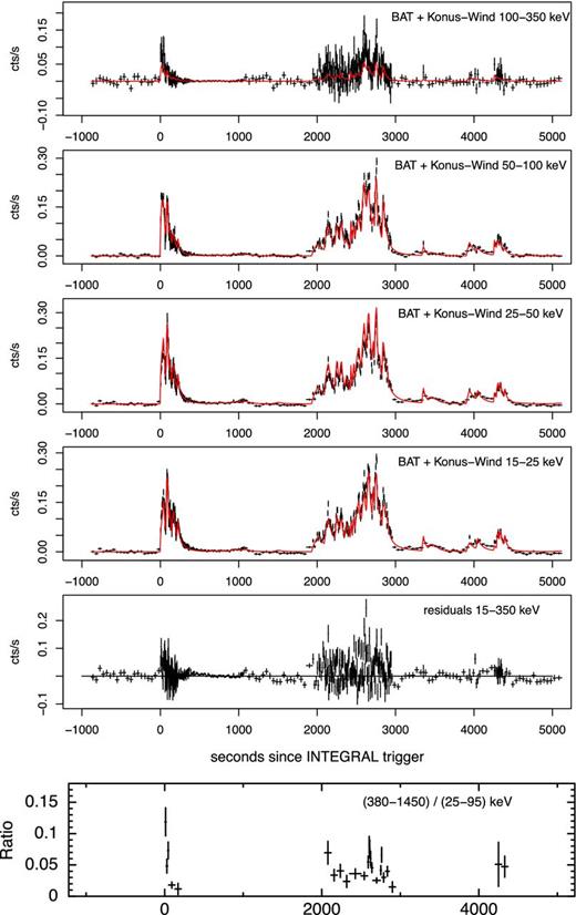
Top four panels: the BAT+Konus-Wind data for the prompt emission in the standard BAT bands, along with the fitted pulse model (red) from Willingale et al. (2010) and residuals. While some fine details of the pulses are not perfectly fitted, the basic shape, time and spectral behaviour of the pulses are well reproduced by our model. The count rates are normalized to the equivalent BAT values in count s−1 per detector values. Bottom panel: the Konus-Wind hardness ratio of counts in the hardest to softest band. Data were binned to a minimum signal-to-noise ratio of 5 in each band, and the data points with large errors during the quiescent periods were removed. The spectral evolution can be clearly seen.
The best-fitting parameters for the 38 pulses. Tpk was not fitted but set by eye. Times are in the observer frame.
| Pulse # | Tpk (s) | Tf (s) | 90 per cent conf range | Γa | 90 per cent conf range | Liso (erg s−1) | 90 per cent conf range |
|---|---|---|---|---|---|---|---|
| 1 | 22 | 33 | 31–37 | 1.19 | 1.12–1.27 | 4.52 × 1050 | 3.98 × 1050–5.10 × 1050 |
| 2 | 41 | 76 | 72–80 | 1.71 | 1.63–1.80 | 2.68 × 1050 | 2.38 × 1050–3.05 × 1050 |
| 3 | 91 | 50 | 49–53 | 1.90 | 1.86–1.93 | 3.97 × 1050 | 3.63 × 1050–4.84 × 1050 |
| 4 | 115 | 129 | 118–139 | 1.95 | 1.77–2.07 | 1.02 × 1050 | 7.96 × 1049–1.39 × 1050 |
| 5 | 168 | 106 | 103–115 | 2.11 | 2.06–2.14 | 1.90 × 1050 | 1.27 × 1050–2.12 × 1050 |
| 6 | 223 | 70 | 67–75 | 2.07 | 2.02–2.12 | 1.14 × 1050 | 9.71 × 1049–1.30 × 1050 |
| 7 | 820 | 217 | 210–225 | 1.63 | 1.58–1.68 | 5.53 × 1048 | 4.69 × 1048–6.47 × 1048 |
| 8 | 1020 | 133 | 132–134 | 1.73 | 1.70–1.74 | 1.34 × 1049 | 1.24 × 1049–1.44 × 1049 |
| 9 | 1120 | 131 | 127–135 | 1.86 | 1.81–1.91 | 9.08 × 1048 | 8.08 × 1048–1.03 × 1049 |
| 10 | 1508 | 207 | 202–215 | 2.11 | 2.05–2.16 | 9.93 × 1048 | 9.19 × 1048–1.08 × 1049 |
| 11 | 2020 | 287 | 267–315 | 1.81 | 1.56–1.92 | 9.50 × 1049 | 7.68 × 1049–1.23 × 1050 |
| 12 | 2143 | 178 | 167–191 | 1.63 | 1.54–1.71 | 1.92 × 1050 | 1.74 × 1050–2.13 × 1050 |
| 13 | 2252 | 127 | 117–139 | 1.73 | 1.59–1.86 | 1.66 × 1050 | 1.40 × 1050–2.00 × 1050 |
| 14 | 2311 | 51 | 45–58 | 1.43 | 1.24–1.63 | 1.59 × 1050 | 1.28 × 1050–2.00 × 1050 |
| 15 | 2374 | 167 | 142–198 | 2.36 | 2.26–2.43 | 1.56 × 1050 | 5.27 × 1049–2.84 × 1050 |
| 16 | 2432 | 34 | 29–44 | 1.18 | 0.95–1.46 | 2.19 × 1050 | 1.48 × 1050–3.02 × 1050 |
| 17 | 2469 | 58 | 51–67 | 1.69 | 1.52–1.91 | 1.50 × 1050 | 1.18 × 1050–2.04 × 1050 |
| 18 | 2532 | 153 | 147–158 | 1.80 | 1.65–1.86 | 2.64 × 1050 | 2.32 × 1050–3.02 × 1050 |
| 19 | 2599 | 132 | 127–139 | 1.26 | 1.20–1.32 | 4.44 × 1050 | 4.11 × 1050–4.81 × 1050 |
| 20 | 2658 | 107 | 103–114 | 1.92 | 1.81–1.98 | 3.30 × 1050 | 2.78 × 1050–3.85 × 1050 |
| 21 | 2719 | 89 | 83–98 | 2.24 | 2.08–2.35 | 2.49 × 1050 | 1.63 × 1050–4.49 × 1050 |
| 22 | 2760 | 27 | 27–28 | 1.49 | 1.43–1.55 | 4.30 × 1050 | 3.97 × 1050–4.65 × 1050 |
| 23 | 2795 | 119 | 108–131 | 1.95 | 1.80–2.25 | 1.37 × 1050 | 9.45 × 1049–2.26 × 1050 |
| 24 | 2842 | 63 | 59–74 | 1.19 | 1.09–1.32 | 3.64 × 1050 | 2.88 × 1050–4.19 × 1050 |
| 25 | 2895 | 100 | 90–113 | 2.78 | 2.43–2.65 | 2.73 × 1050 | 4.23 × 1049–8.49 × 1050 |
| 26 | 3356 | 94 | 72–132 | 1.96 | 1.48–2.31 | 8.62 × 1049 | 4.88 × 1049–1.79 × 1050 |
| 27 | 3517 | 146 | 122–181 | 2.34 | 1.77–3.01 | 4.32 × 1049 | 2.45 × 1047–1.19 × 1050 |
| 28 | 3943 | 162 | 150–183 | 1.28 | 1.07–1.51 | 9.63 × 1049 | 7.42 × 1049–1.29 × 1050 |
| 29 | 4050 | 157 | 143–172 | 2.25 | 1.91–2.68 | 8.16 × 1049 | 2.68 × 1049–2.16 × 1050 |
| 30 | 4261 | 61 | 42–85 | 0.69 | 0.21–1.24 | 1.96 × 1050 | 9.11 × 1049–4.41 × 1050 |
| 31 | 4309 | 67 | 60–80 | 2.02 | 1.59–2.28 | 1.05 × 1050 | 6.87 × 1049–2.17 × 1050 |
| 32 | 4339 | 81 | 68–92 | 2.22 | 1.77–2.59 | 1.11 × 1050 | 3.59 × 1049–2.93 × 1050 |
| 33 | 4396 | 73 | 62–86 | 2.31 | 1.84–2.99 | 9.57 × 1049 | 4.34 × 1049–4.69 × 1050 |
| 34 | 5120 | 336 | 325–343 | 2.37 | 2.33–2.41 | 4.98 × 1048 | 4.72 × 1048–5.32 × 1048 |
| 35 | 7259 | 1305 | 1287–1323 | 1.73 | 1.67–1.77 | 1.50 × 1049 | 1.37 × 1049–1.73 × 1049 |
| 36 | 10 970 | 619 | 531–830 | 2.62 | 2.29–2.93 | 5.37 × 1047 | 3.12 × 1047–9.36 × 1047 |
| 37 | 11 439 | 551 | 527–574 | 2.78 | 2.66–2.90 | 4.70 × 1047 | 3.89 × 1047–5.72 × 1047 |
| 38 | 12 036 | 989 | 637–1464 | 2.57 | 0.28–3.50 | 2.27 × 1047 | 6.65 × 1046–2.47 × 1048 |
aΓ is the spectral photon index of the pulse, this is constant for that pulse, whereas Epk evolves with time. See Willingale et al. (2010) for details.
Since the publication of Willingale et al. (2010), one of us (RW) has fitted the BAT pulses and XRT flares for 127 GRBs with a redshift and early XRT data up to 2011 May, so we compared the results for GRB 130925A with that sample (which does not include any of the other ultralong GRBs). GRB 130925A required 38 distinct pulses, substantially more than any other GRB in our sample (Fig. 5, top). Not surprisingly given the duration of GRB 130925A, most of these pulses peak at a rest-frame time much later than the generality of GRB pulses (Fig. 5, middle); also the pulses are longer (in the GRB rest frame) than most prompt pulses, although within the distribution found from the population at large (Fig. 5, bottom). For the pulse population as a whole, a correlation is seen between the rest-frame Tpk and Tf values (the pulse peak time and duration, respectively, Fig. 6, top), and an anticorrelation exists between the rest-frame duration and the isotropic-equivalent peak luminosity of the pulses (Fig. 6, bottom). As Fig. 6 shows, the pulses in GRB 130925A are consistent with the first of these correlations, but are a factor of ∼5–10 more luminous for their durations than is typical for GRB pulses. In summary, the prompt emission pulses are largely consistent with what we see in most GRBs, except that there are more of them, extending to later times than normal, and they carry more energy than typical pulses of the same duration.
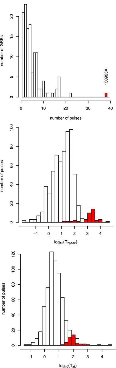
Comparison of the prompt emission properties of GRB 130925A with the 127 GRBs with known redshift observed by Swift-BAT and XRT up to 2011 May. GRB 130925A is in red. Top: the distribution of the number of pulses needed to model the prompt emission. Middle: the distribution of the peak time of the pulses in the GRBs’ rest frame. Bottom: the distribution of the duration of the pulses in the GRBs’ rest frame. The number of pulses and their peak times are unusually large compared to the population of GRBs as a whole. The pulse durations in GRB 130925A are at the high end of the overall distribution, although not inconsistent with the general range.
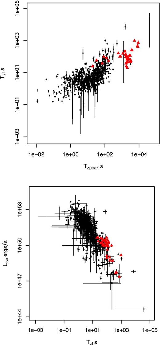
Comparison of the prompt emission relationships of GRB 130925A with the 127 GRBs with known redshift observed by Swift-BAT and XRT up to 2011 May. GRB 130925A is in red. Top: the pulse duration plotted against the pulse peak time (both in the GRBs’ rest frames); GRB 130925A lies along the correlation seen for the population at large. Bottom: the isotropic-equivalent luminosity of the pulses against the pulse duration (rest frame). The pulses for GRB 130925A tend to be longer for their luminosity (i.e. more energetic) than the generality of GRB pulses.
THE SPECTRALLY EVOLVING X-RAY AFTERGLOW
GRBs show a wide variety of X-ray afterglow behaviour; however, one thing they all have in common is that almost no evidence for late-time spectral evolution has been reported12 (e.g. Butler & Kocevski 2007; Evans et al. 2009). However, the XRT hardness ratio of GRB 130925A, after the flaring behaviour has subsided, shows a strong spectral evolution from T0 + 20 to T0 + ∼700 ks (Fig. 7). Fitting the hardness ratio (HR) time series from T0 + 20 ks with a broken power law (i.e. HR ∝ t−ζ up to the break, after which the HR is constant) yielded a fit with χ2 = 23.2 (ν = 31). The break time, where the evolution ceased, is (8.3|$^{+2.1}_{-2.6}$|) × 105 s, and |$\zeta =0.256^{+0.030}_{-0.026}$| (errors at 1σ) i.e. the source is getting softer with 10σ significance! A similar behaviour has been reported in one previous burst: GRB 090417B for which the late-time X-ray data was interpreted by Holland et al. (2010) as scattering of the prompt emission off a dust screen, rather than emission from an external shock.
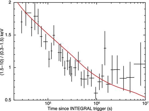
Swift-XRT hardness ratio time series, showing the ratio of counts in the 1.5–10 and 0.3–1.5 keV bands. The data shown begin at T0 + 20 ks (i.e. once the prompt emission and flaring had ceased). The strong hard-to-soft evolution can be clearly seen. The red line shows the hardness ratio predicted by the dust-scattering model (Section 4.2).
We attempted to model the late-time13 X-ray emission of GRB 130925A in two ways: first as an external shock, and then using dust scattering.
The X-ray afterglow as an external shock
In the best-fitting model (with spectral evolution), the isotropic-equivalent 0.3–350 keV peak (i.e. at t = ta) luminosity of the afterglow is |$L_{\rm ag}=5.3^{+9.7}_{-3.6} \times 10^{46}$| erg s−1 and the total 0.3–350 keV fluence of the afterglow is |$3.5^{+6.5}_{-2.4} \times 10^{51}$| erg (this is measured by integrating the model over all times). This means GRB 130925A has one of the lowest ratios of afterglow to prompt fluence seen in the sample of 127 GRBs analysed (see Fig. 8).
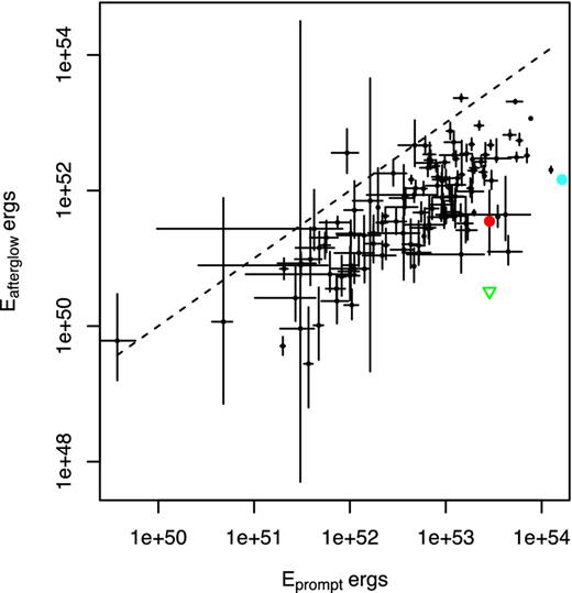
The distribution of afterglow fluence against prompt fluence for the long GRBs in our sample. The red point shows the afterglow fluence of GRB 130925A: the Eafterglow/Eprompt is lower than for most bursts. The green triangle is the upper limit on external-shock emission in the dust-scattering model. In this case, the external-shock emission must be significantly lower, as a fraction of the prompt emission, than for any other GRB. The cyan point is the ultralong GRB 121027A.
In order to investigate in more detail possible physical causes of the spectral evolution, we extracted a series of spectra between T0 + 27.8 and T0 + 2000 ks (i.e. from the first XRT snapshot after the flaring had ended until the spectral evolution had stopped), producing one spectrum every 250 accumulated counts, giving 27 spectra in total. We then fitted these spectra simultaneously in xspec. We initially fitted an absorbed power law, with two photoelectric absorption components. The first was a phabs fixed at the Galactic value of 1.7 × 1020 cm−2, the second was a zphabs with a redshift fixed at 0.348, and the column density free, but tied between the 27 spectra (i.e. time-invariant). The power-law photon index and normalization were free parameters. The best fit gave |$\mathcal {W}=4122$|, for 4703 degrees of freedom. This spectrum has no physical interpretation within the synchrotron model, but serves as a baseline to compare other models with. These fits showed no evidence for the high-energy residuals reported by Bellm et al. (2014).
We next tried replacing the power law with a broken power law, with the photon index above the break fixed to be 0.5 higher than the photon index below the break. Only the low-energy slope, break energy and normalization were allowed to vary between the fits. This reproduces the spectral evolution expected if the synchrotron cooling frequency is moving through the XRT bandpass. This gave a worse fit than the power-law fit (|$\mathcal {W}=4426$|, ν = 4758) and the break energy was extremely variable, showing no sign of the steady evolution expected of the synchrotron cooling frequency.
We also tried fitting a power law plus blackbody, to investigate whether some evolving optically thick component could be present and modifying the fit (e.g. Campana et al. 2006; Starling et al. 2013). In this model, the power-law photon index was tied between spectra; we used a zbbody model (i.e. a blackbody, with the temperature set in the GRB rest frame) with the redshift fixed at 0.348. The best fit gave |$\mathcal {W}=4255$| (ν = 4675), again this is worse than simply having an evolving power law. Furthermore, the blackbody temperature was highly variable with no steady evolution and frequently it tended to extreme values (i.e. 10−4 or 200 keV: the model limits).
Since this paper was posted on arXiv, Piro et al. (2014) have also published an analysis of the data, in which they claim the detection of blackbody emission during this interval of strong spectral evolution, in contrast to our result above. However, they fitted a single Swift spectrum (‘A1’ in their paper) covering the interval T0 + 20–300 ks, during which the spectrum evolves significantly (Fig. 7); whereas we used multiple spectra (with good S/N) during this interval. Fitting a single, non-evolving component to a strongly evolving spectrum sometimes results in spurious extra components being needed to reproduce the spectrum, but these are artefacts of the inadequate model. Our approach of time-slicing during this strong evolution is less prone to such effects, thus we reiterate our quantitative result from the previous paragraph: the spectral evolution observed in this burst cannot be modelled as a constant-spectral power law with an evolving blackbody.
In summary: to model the late-time X-ray emission as arising from an external shock, we need to add a late-time break, and we need to impose spectral evolution, the physics of which we cannot account for with the confines of the external-shock model: we therefore suggest than an alternative explanation is needed for the late-time X-ray data.
The X-ray afterglow as dust scattering
Scattering of X-rays from a GRB by dust in our Galaxy has been detected previously (Vaughan et al. 2004). The formation of an afterglow by the scattering of prompt X-rays by dust in the host galaxy was considered by Klose (1998) and modelled by Shao & Dai (2007), who were able to reproduce the morphology of X-ray afterglow light curves. This work was then extended by Shen et al. (2009) who considered the spectral predictions of the dust model (see also Shao & Dai 2007) and found that dust scattering causes the afterglow to get softer with time, in contrast with observations. One counter-example is GRB 090417B, which does show significant softening during the afterglow, and Holland et al. (2010) modelled that GRB using the dust scattering model. Here, we follow the same methodology to consider whether the spectral evolution of GRB 130925A (which is significantly stronger than that of GRB 090417B) could be the result of dust scattering.
The quality of the fit to the multiband light curve using the dust scattering model for the afterglow was about the same as that achieved using the standard afterglow model (Section 4.1): there were 120 free parameters (one less than the standard model) with 3990 data points giving |$\chi ^{2}_{\nu }=3.36$| (this includes the contribution from the pulse model fit to the prompt data). The best-fitting values and 90 per cent confidence ranges for all the fitted dust parameters are given in Table 7. As τ0 is slightly greater than unity, the single-scattering approximation we have used is not strictly valid; however, the impact of this simplification is expected to be small.
The best-fitting parameters to model the late-time X-ray emission as dust scattering of the prompt emission.
| Parameter | Value | Error range |
|---|---|---|
| τ0 | 1.16 | 1.10–1.35 |
| a− μm | 0.021 | 0.0001–0.040 |
| a+ μm | 0.285 | 0.250–0.400 |
| q | 5.0 | 4.6–5.8 |
| Rm pc | 77 | 72–175 |
| Rr pc | 2000 | 1060–3250 |
| Parameter | Value | Error range |
|---|---|---|
| τ0 | 1.16 | 1.10–1.35 |
| a− μm | 0.021 | 0.0001–0.040 |
| a+ μm | 0.285 | 0.250–0.400 |
| q | 5.0 | 4.6–5.8 |
| Rm pc | 77 | 72–175 |
| Rr pc | 2000 | 1060–3250 |
Whereas for the external-shock model, we had to artificially add a late break and spectral evolution to the model in order to fit the data, the dust scattering model fits all the pertinent features of the afterglow naturally: the luminosity of the plateau, the initial slow decay from the plateau, the soft spectrum at the start of the decay and the evolution of the spectrum during the decay and the late break (Figs 9 and 10).
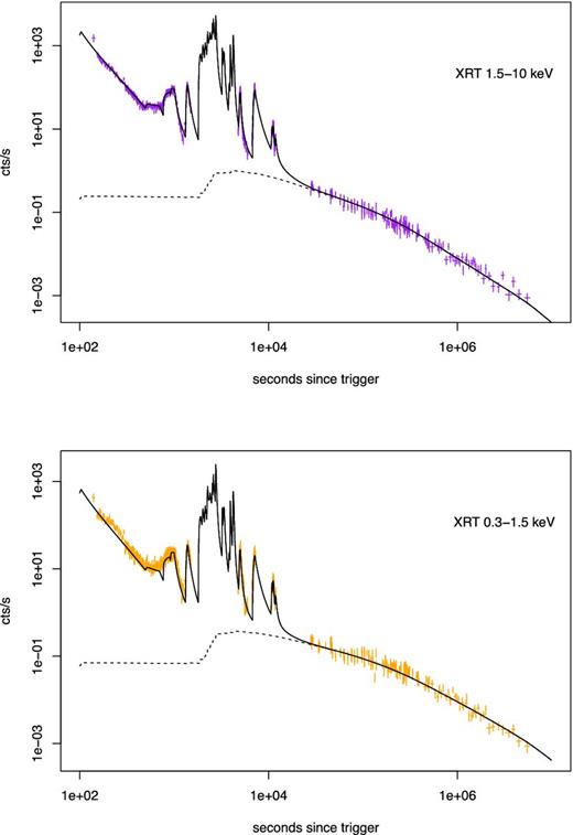
The dust model fit to the late-time XRT data GRB 130925A. The solid line shows the model previously fitted to the prompt emission, plus the dust model. The dust model is shown as the dashed line. The top and bottom panels show the hard and soft XRT bands, respectively, illustrating the good fit of the dust models to both bands.
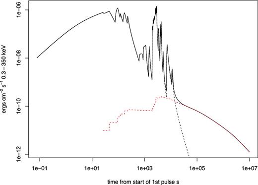
The best-fitting prompt emission and dust scattering model, in flux units over the 0.3–350 keV band. The stepping behaviour in the rise of the dust echo shows the injection of each prompt pulse, which is treated as instantaneous.
The combination of these features provides a useful constraint on all the fitted parameters. The optical depth, τs and the upper size limit, a+ dominate the plateau and early decay behaviour while the lower size limit, a− and index q set the overall decay. The 90 per cent range for a− indicates an upper limit and, not unreasonably, that the grain size distribution probably extends down to very small values. The best-fitting value for the size index, q = 5, we derived here is significantly larger than the canonical value of q = 3.5 usually adopted (Mathis, Rumpl & Nordsieck 1977), although Predehl & Schmitt (1995) find a median value of q = 4.0 from analysis of dust scattering halo distributions observed in our Galaxy. The upper limit to the grain size, a+ = 0.29 μm is consistent with values obtained in similar studies (e.g. Predehl & Schmitt 1995; Holland et al. 2010). The minimum distance, Rm and radial spread, Rd set the curvature and position of the late break seen in the light curve at ∼80 ks The fitting clearly favours a distribution of dust along the line of sight, with a depth of at least 1 kpc, rather than a single thin dust layer. Furthermore, the model approximately reproduces fairly well the correct spectral index and spectral evolution for the afterglow of GRB 130925A.
Fig. 9 shows the fitted XRT light curves. Fig. 10 shows the model 0.3–350 keV flux for both the prompt and afterglow component from the start of the burst through to the final decay.
We can estimate the expected optical extinction, AV, using the relation given by Draine & Bond (2004), τs/AV ≈ 0.15(E/1 keV)− 1.8, and we can further estimate the associated total hydrogen column using the relation derived by Willingale et al. (2013) for our Galaxy, NHtot/AV = 3.2 × 1021 cm−2. These give AV = 7.7 mag and NHtot = 2.5 × 1022 cm−2. Both these relationships were derived using data from the Milky Way but there is substantial evidence that the dust properties of GRB hosts are different from the Milky Way or galaxies in our neighbourhood (see the discussion in Shen et al. 2009); an Small Magellanic Cloud-like metallicity would give AV ∼ 6.2. Despite these caveats the value of NHtot derived from the dust-echo afterglow model is comparable to the intrinsic NH = (1 ± 0.1) × 1022 cm−2 at z = 0.348 derived from the late-time XRT spectrum. Thus, the dust required to produce the observed afterglow by X-ray scattering alone is consistent with the intrinsic absorbing column required to fit the X-ray spectrum. Also note that the galaxy-integrated colours are consistent with a dusty galaxy (Section 2.1).
If substantial dust is present near the GRB, we may expect to observe evidence of dust destruction. According to Waxman & Draine (2000), dust destruction occurs out to radii of about 10 pc from the GRB, while Fruchter, Krolik & Rhoads (2001) suggested that X-ray effects can destroy dust out to radii of ∼100 pc. According to Table 7, the dust screen in GRB130925A extends from ∼80–2000 pc; thus, we expect only a small amount, if any, of the dust to be destroyed, and that at the inner edge of the screen: any visible signature of this is likely to be weak and attenuated by its passage through the screen. Note that, should any dust destruction occur, this would reduce the optical extinction along the line of sight, but not the absorption column inferred from X-rays.
The X-ray afterglow as an external shock and dust scattering
While the dust emission appears to fit the observed late-time data, we expect there to be some contribution from an external shock, unless the CBM is of an abnormally low density. We thus added a standard afterglow component (Section 4) to the dust model. The time of the plateau start (i.e. ta) was fixed at 18.9 ks (as obtained in the fit without dust): values earlier than this cannot be constrained due to the brightness of the prompt emission. The photon index of the standard afterglow was fixed at 2.0, the median value obtained for all afterglows fitted by Willingale et al. (2010). The best fit was obtained with no external-shock component. The inclusion of any emission from this component increased χ2, because the spectrum of the external shock was much harder than that observed (which is well reproduced by the dust model). The peak afterglow flux permitted by the fit at the 90 per cent confidence level was 7.04 × 10⁻¹² erg cm−2 s−1 (at T0 + 18.9 ks). Integrating this external-shock component over all times gives us a 90 per cent confidence upper limit of Eiso, afterglow < 3.3 × 1050 erg for the total fluence of the external shock.15 This is plotted against the prompt fluence as a green triangle in Fig. 8, which shows that the energy radiated in the external shock, as fraction of the prompt energy, is lower than seen for any other GRB.
We therefore consider it likely that the X-ray ‘afterglow’ emission from GRB 130925A is in fact the prompt emission being scattered into our line of sight by dust in the GRB host galaxy, rather than emission from the standard external shock seen in typical GRBs.
Spectral evolution in other GRBs
Strong spectral evolution has now been found in the afterglows of GRBs 090417B and 130925A. To investigate how widespread this phenomenon is, we systematically studied all GRB afterglows detected by Swift-XRT up to GRB 131002A for which the observations had a time base of at least 20 ks.
We excluded the first 3 ks after the trigger (where the data may be affected by the prompt and high-latitude emission) and the times of any flares identified by the automatic fitting in the online XRT catalogue16 (Evans et al. 2009); we then fitted a power law to the hardness ratio time series. For each fit, we calculated the significance of the power-law index deviation from 0 (i.e. ζ/σζ, where HR ∝ t−ζ); a histogram of these values is given in Fig. 11. There is an excess of objects with a spectral softening over time present at the ∼2σ level, and 16 objects with evolution seen at the 5σ level. We manually examined all of the latter; in five cases, we found that the evolution was caused either by flares which had not been adequately filtered out, or by a poorly sampled hardness ratio, where a single errant bin was dominating the fit. However, bona fide spectral evolution was found in GRBs 130907A, 110709A, 100621A, 090404, 090417B, 090201, 081221, 080207 and 060218, as well as GRB 130925A.17 For these GRBs, we created a series of spectra, starting a new one every ∼250 counts, and fitted them with an absorbed power law with the absorption component fixed, in a manner analogous to what we did for GRB 130925A in Section 4.1. For some of these GRBs, the spectral evolution seen in the hardness ratio did not begin until part way through the light curve, and a broken power law gave a better fit to the HR evolution; in those cases, we only took spectra from the time of the break onwards.
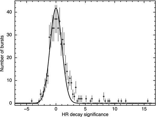
The distribution of the significance, in σ, of any hardness ratio variation, for 672 XRT GRB afterglows up to GRB 131002A. There is an excess of objects showing hard-to-soft spectral evolution; we investigated those with >5σ significance in more detail.
The time evolution of the photon index for these bursts is shown in Fig. 12. The general behaviour of the bursts is similar to that seen in GRB 130925A, although the latter is softer than the majority of even these bursts. The only burst with a softer spectrum is GRB 060218, which was an atypical burst in which a strong thermal component was detected, that evolved to lower temperatures (Campana et al. 2006). It has also been suggested by Sparre & Starling (2013) that GRB 100621A may have a thermal component; however, the presence of that component is by no means certain, and appears to be limited to the early-time data, thus is unlikely to be the cause of the late-time evolution we report here.
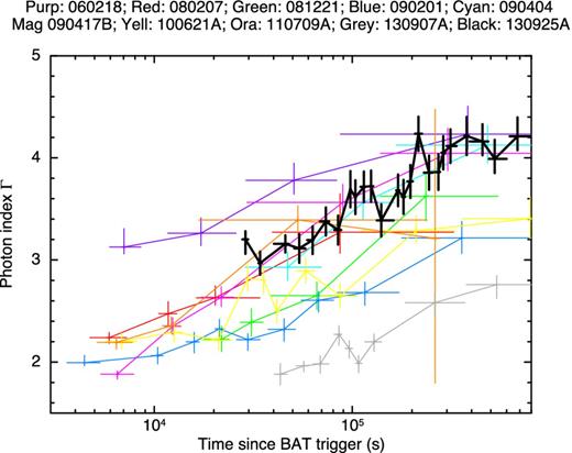
The spectral photon index as a function of time, for the GRB afterglows which show spectral softening. The photon index is derived from fitting absorbed power-law models to a series of time-resolved spectra.
The afterglow light-curve morphology of this collection of bursts is heterogeneous; with such a small sample, it is impossible to draw firm conclusions; however, the distribution of morphologies is similar to that reported by Evans et al. (2009) for the first 327 Swift-detected GRBs. This makes it unlikely that all of these GRBs have late-time emission caused purely by dust with no contribution from an external shock, as we postulate for GRB 130925A, but dust scattering may contribute to their emission. We therefore looked in the literature and GCN circulars for the eight GRBs with spectral softening (excluding GRB 060218) to see if the GRBs are reported either as being ‘dark’ bursts (e.g. Jakobsson et al. 2004; van der Horst et al. 2009) or significantly reddened bursts, both of which are likely indications of significant dust in the host galaxy. We found such evidence for six of the GRBs: GRB 080207 (Krühler et al. 2012; Perley et al. 2013); GRB 081221 (Melandri et al. 2012); GRB 090201 (Melandri et al. 2012); GRB 090404 (Perley et al. 2013); GRB 100621A (Melandri et al. 2012; Greiner et al. 2013) and GRB 130907A (Schmidl et al. 2013). Additionally, Hunt et al. (2014) reported significant dust in GRB 090417B. The remaining GRB (GRB 110709A) has only upper limits in the optical band, which may also indicate the presence of dust. These results support a generalization of our explanation for the spectral evolution of GRB 130925A, namely that spectral softening of the X-ray afterglow of a GRB is the result of dust scattering of the prompt emission.
Note that this conclusion cannot necessarily be inverted to argue that a highly extincted optical afterglow should correspond to a spectrally evolving X-ray afterglow: this is only the case when the dust echo is of significant brightness relative to the external shock, and the redshift is ≲1.5 (at higher redshift, the bulk of the dust-echo fluence lies below the XRT energy band). We selected all GRBs within this redshift range, and plotted the index of the HR evolution, ζ ± σζ, against the ratio, Eafterglow/Eprompt, coloured according to the intrinsic absorption column (according to the late-time spectral fits in the XRT Spectrum Repository;18 Evans et al. 2009). We searched for any examples with a high (>1022 cm−2) column and faint afterglow, but no evidence for spectral evolution; objects which would argue against our interpretation. We found no such cases (Fig. 13). We therefore suggest that the range of light-curve morphologies seen in our sample of softening afterglows indicates the differing relative strengths of the dust echo and external shock. GRB 130925A, with an exceptionally weak external shock (Section 4.3) is the most extreme example.
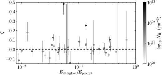
The hardness ratio temporal evolution index (ζ) as a function of the ratio of prompt-to-afterglow energy release and intrinsic absorption. The ratio Eafterglow/Eprompt refers to the integrated fluence of the afterglow and prompt models. If any objects were seen with a low Eafterglow/Eprompt ratio and either high intrinsic column and no spectral evolution; or spectral evolution but a low intrinsic column, this would contradict our model that spectral evolution is indicative of dust in the host galaxy. No such bursts are seen, supporting this model. Note that GRB 130925A is not included in this plot.
DISCUSSION
GRB 130925A was a very long GRB, with high-energy emission (E > 15 keV) detected until ∼5 ks after the initial trigger, and the prompt emission dominating the light curve until ∼20 ks after the trigger. Three other GRBs (101225A, 111209A and 121027A) also show such long-lived activity, prompting some authors (Gendre et al. 2013; Levan et al. 2014) to suggest that these belong to a new category of ‘ultralong’ GRBs. There is no formal definition of such objects, but the long duration of GRB 130925A clearly places it in this category. These authors propose several possible causes of these ultralong GRBs: most notably a tidal disruption event (TDE) in which a star is destroyed and partially accreted by a massive black hole at the centre of a galaxy; and a GRB from the collapse of a blue supergiant (see also Nakauchi et al. 2013; Stratta et al. 2013), rather than the Wolf–Rayet progenitor associated with ‘normal’ long GRBs Woosley (1993). However, the identification of these GRBs as a new class of object is not certain. Due to the low-Earth orbit of the Swift and Fermi satellites, it is difficult to accurately measure the duration of such long GRBs with these satellites. Indeed, for GRB 130925A we find that roughly 75 per cent of the fluence occurred during the second emission episode (T0 + 2–3 ks, Section 3), which was completely missed by Swift and Fermi. Similarly, for GRB 121027A a significant proportion of the emission took place while Swift was not observing it (Starling et al., in preparation), and for GRB 111209A the Konus-Wind light curve19 shows that the emission continued for about 3 ks after BAT finished observing. Thus, we cannot simply determine the distribution of GRB durations based on the Swift-BAT results.
Zhang et al. (2014) attempted instead to define the duration of the burst as the maximum time over which emission from processes internal to the jet (i.e. prompt emission or X-ray flares) are seen. The distribution of this duration has broad long-duration tail, perhaps suggestive of a single population of objects. Zhang et al. (2014) suggested that this could be interpreted as indicating the duration of the GRB central engine activity, which means that the GRB central engine is still active at the time a flare is detected. Late-time X-ray flares (e.g. Curran et al. 2008) could, however, arise from internal shocks between two shells of similar Lorentz factor, in which case the time of collision could be much later than the time at which they were ejected by the central engine; although Lazzati & Perna (2007) considered this scenario and suggested it was more likely that the central engine was indeed still active at this time. Nonetheless, there is a significant difference between these objects with late flares – where the central engine apparently turns off for a long period of time, and then emits a single, late-time flare – and the ultralong bursts where the central engine is active and highly energetic for a sustained period.
GRB 130925A is the first of these ultralong bursts to which the pulse modelling of Willingale et al. (2010) has been applied. Fig. 5 showed that while the durations of the individuals pulses lie within with the distribution seen from the GRB population at large, the number of pulses and their peak times do not. To determine whether this is the result of the selection biases referred to above (i.e. we cannot detect pulses when Swift is not observing the burst), we plot in Fig. 14 the distribution of the pulse times divided by the times at which Swift's first observation of the GRB ended. This shows values only for GRBs shown in Figs 5–6 with GRB 130925A excluded. Whereas Fig. 5 (centre panel) shows that the distribution of flare peak times drops off sharply at around T0 + 100 s, Fig. 14 shows that there is no sharp drop corresponding to the end of the Swift observation. It is highly improbable that GRBs systematically return to quiescence a few minutes after the trigger, and then flare up again when Swift has slewed away (without triggering any other GRB satellite during this later episode). We therefore suggest, given the lack of GRBs with peak times or numbers of pulses between those of GRB 130925A and the bulk of the distribution, that the prompt emission of GRB 130925A and the other ultralong bursts, are not consistent with the tail of some continuous distribution of behaviours seen in ordinary long GRBs (as suggested by Virgili et al. 2013).
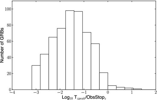
The distribution of the time of GRB pulses (Tzpeak) relative to the time Swift slewed away from the burst (ObsStopz). The GRBs in this plot are those from Figs 5–6, with GRB 130925A excluded. The lack of a sharp drop at Tzpeak/ObsStopz = 1 shows that the absence of late-time pulses in most long GRBs is not an observational selection effect.
In Fig. 15, we show the Swift-XRT light curves of all four of the candidate ultralong GRBs, converted to luminosity in the rest-frame 0.3–10 keV band. There are strong similarities between them, especially at around T0 + ∼20 ks, where the prompt emission appears to cease. We thus interpret GRB 130925A as belonging to the class of ultralong GRBs and that these are a distinct class of objects. We now consider the plausibility of both the TDE and GRB scenarios for GRB 130925A.
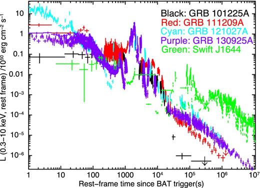
The rest-frame X-ray light curves of the ultralong GRBs identified by Levan et al. (2014), and GRB 130925A. Swift J1644 is also shown for comparison. The energy band is 0.3–10 keV in the rest frame. For all but GRB 130925A only the BAT event data and the XRT data are shown, k-corrected from the Swift Burst Analyser (Evans et al. 2010) and Light Curve Repository (Evans et al. 2007, 2009), respectively. For GRB 130925A, the Konus-Wind data are also shown; these provide the data around 1000–3000 s. The similarity between the four ultralong bursts can be seen, as can the difference between these and the TDE candidate Swift J1644.
Is GRB 130925A a TDE?
If GRB 130925A is a TDE, we would expect it to be located at the centre of the galaxy, where the supermassive black hole should lie. However, the HST observations show it to lie 0.12 arcsec (∼600 pc) away from the galaxy nucleus (Tanvir et al. 2013). Those same observations show the galaxy to be somewhat distorted, suggestive of a recent merger; in such a case, the galaxy could potentially host two such black holes which have not yet had time to merge and return to the centre of mass (e.g. Milosavljević & Merritt 2001; Comerford et al. 2013), thus the offset does not rule out the TDE scenario.
As Levan et al. (2014) pointed out, a bigger problem faced by the TDE scenario is that of time-scales: for disruption of a main-sequence star by a 106 M⊙ black hole Lodato & Rossi (2011) predicted that the X-ray emission would show a rise or plateau lasting ∼100 d or more, whereas for GRB 130925A the light curve is steadily decaying by ∼0.3 d after the trigger.20 Krolik & Piran (2011) considered the case of a white dwarf being tidally disrupted by a lower mass (104 M⊙) black hole; as Levan et al. (2014) noted, their equation (5) represents the shortest time-scale on which we may see variations. Equating this to the ∼2 ks gap between the burst episodes requires a 600 (2 × 10⁴) M⊙ black hole for a 1 (1.4) M⊙ white dwarf. These values are not impossible, but clearly to explain the observed time-scale in terms of a TDE requires either a relatively low-mass black hole, or high-mass white dwarf.
The predicted peak brightness of TDEs is also a problem. Levan et al. (2014) commented that the ultralong GRBs are much more luminous (during their prompt emission) than Swift J1644.3+573451, which is believed to be a TDE detected by Swift (Bloom et al. 2011; Burrows et al. 2011; Levan et al. 2011),21 and this is clear from Fig. 15. Lodato & Rossi (2011) performed numerical simulations of TDEs for a range of black hole masses, and report peak isotropic luminosities of ∼1044 erg s−1 (see their fig. 7, for example). The average luminosity of GRB 130925A during the prompt phase is ∼Eiso/2200 (i.e. the prompt energy release divided by the approximate ‘on time’ of the burst) ≈1.3 × 1050 erg s−1, which is many orders of magnitude above the predicted TDE peak. To reconcile these numbers by assuming that in GRB 130925A, the radiation we see is beamed requires a jet opening angle of ∼0| $_{.}^{\circ}$|07. While this may not be impossible, it would mean that for every TDE we detect, about 107 are beamed away from us. Given that Swift has detected four ultralong GRBs in 9 yr out to z = 1.773, i.e. a volume of 4.9 × 10⁵ Mpc3, this implies a TDE rate of ∼9 yr−1 Mpc−3, greatly in excess of the predicted rate of 10−5 yr−1 Mpc−3 (Wang & Merritt 2004). Further, due to its shortness (for a TDE) such beaming reduces the overall fluence of the TDE to 2.2 × 1047 erg,22 which corresponds to the accretion of 10−6 M⊙ of material (assuming 10 per cent radiative efficiency, Lodato & Rossi 2011); whereas Ayal, Livio & Piran (2000) suggest that about 10 per cent of the stellar mass will be accreted.
Another difficulty with the TDE scenario is the lack of fallback emission. Once the initial disruption event is over, some fraction of the stellar matter is accreted on to the black hole, producing a light curve which decays as t−5/3 (e.g. Rees 1988; Evans & Kochanek 1989; Phinney 1989). However, the late-time emission in GRB 130925A is best modelled by dust scattering of the early emission, not fallback emission. We therefore tried to determine limits on the possible emission from this fallback. In Section 4.3, we determined the upper limit on the energy from a standard GRB afterglow to be 3.3 × 1050 erg. Assuming 10 per cent radiative efficiency, this corresponds to the accretion of just ∼2 × 10⁻³ M⊙ of material, much lower than predicted by Ayal et al. (2000). Given that the standard afterglow model we used to derive the limit on the afterglow emission decays more slowly than t−5/3 (i.e. TDE decay), the limit on emission from fallback accretion is even lower than 2 × 10⁻³ M⊙.
We therefore consider it very unlikely that GRB 130925A can be explained in the TDE paradigm.
Is GRB 130925A a GRB collapsar?
There are two difficulties to interpreting GRB 130925A as a normal long GRB: its long-lived emission at high energies (E > 15 keV, Section 3.1) and the low luminosity of the external-shock emission (Section 4.3). The former is, by definition, common to the ultralong GRBs, and Gendre et al. (2013), Nakauchi et al. (2013) and Levan et al. (2014) have suggested that it could be explained by the collapse of a blue supergiant, as opposed to the smaller Wolf–Rayet progenitor of normal long GRBs. Considering the lack of external-shock emission, Fig. 15 shows that GRB 101225A also has little or no afterglow emission. GRBs 121027A and 111209A have similar late-time X-ray light curves to GRB 130925A, but there is no sign of spectral softening (the signature of dust scattering), implying that in those bursts the X-ray emission arises from the standard external forward shock. However, the similarity of their light curves with GRB 130925A tells us that the ratio of prompt-to-afterglow fluence for those GRBs must be similar to GRB 130925,23 i.e. all four of the ultralong GRBs have afterglows which are underluminous compared to their prompt emission, when compared with the population of normal long GRBs.
We now consider specifically the lack of external-shock emission in GRB 130925A. For a standard afterglow, the brightness of the external shock depends on the microphysical parameters of the shock, which cannot be constrained by the XRT limit alone. Fortunately, the radio data from Bannister et al. (2013) at T0 + 15 d, are close in time to the second-epoch HST data which give F1.6 μm ∼ 0.6 μJy (Tanvir et al., in preparation). From the Swift Burst Analyser (Evans et al. 2010), the X-ray flux density at 10 keV at this time was ∼10− 4 μJy, with the contribution from the external shock being at least a factor of 3 lower (Section 4.3). A rough spectral energy distribution (SED) constructed from these data does not allow us to place stringent constraints on the afterglow properties, but is consistent with a synchrotron model, where the electron distribution index p = 2.2 (where N(E) ∝ E−p) and νm < νradio, HST < νc < νx (where νm is the synchrotron peak frequency, νc is the cooling frequency, and νradio, HST, x are the frequencies of the radio, HST and XRT emission, respectively). Using the equations of Granot & Sari (2002) this loose constraint on νc gives 10−4 ≲ n ≲ 1.5 cm−3, but also predicts an X-ray flux significantly higher than measured. In order to bring the predicted flux into agreement with the observations, we have to reduce the kinetic energy of the outflow to ∼5 × 1051 erg. Alternatively, we can in principle suppress the flux if the magnetic parameter of the shock, ϵB, is very low (e.g. Uhm & Beloborodov 2007); however, in order to keep νc between the optical and X-ray bands while reducing ϵB requires the circumburst density to increase, and only unphysical values of ϵB and n can reproduced the observed fluxes.
An alternative explanation is that the optical and radio emission comes not from the external forward shock, but from a reverse shock (Genet et al. 2007; Uhm & Beloborodov 2007; Hascoët et al. 2011). To fit the rough SED we produced above, we again require νm < νradio,HST < νc < νx, but in this case the normalization of the SED depends on the distribution of densities and Lorentz factors behind the shock (see the papers just cited for details); the modelling of which is beyond the scope of this paper. For the reverse shock model to work, it is still necessary to suppress the emission from the forward shock. The authors above do this by requiring ϵB to be low (∼10−7) in the external shock. Unlike in the situation described above for the forward shock, this is attainable because we have no observational constraints on the shape of the spectrum from the (suppressed) forward shock.
Thus, if GRB 130925A is a GRB, we need to explain either why it should radiate a greater proportion than normal of its energy during the prompt phase, or have an unusually low magnetic energy in the external shock. As noted above, the low luminosity of the afterglow compared to the prompt emission appears to be common to all four ultralong GRBs. This raises the possibility that some mechanism related to the burst duration also increases the fraction of energy radiated during the prompt phase; that is the fraction of the energy in the outflow which is converted to radiation. It is tempting to interpret the bottom panel of Fig. 6 – which shows that the pulses in GRB 130925A tend to be longer lived for their luminosity than the general population of pulses – as supporting this idea. However, this does not tell us anything about the efficiency with which the energy contained in the interacting matter is radiated. The fraction of the initial energy radiated as prompt emission depends not only on the mechanism by which interactions in the outflow dissipate energy, but also on how much of the outflow is involved in such interactions. In the standard internal-shock model, interactions occur when two shells of material are emitted at times t2 > t1 with Lorentz factors Γ2 > Γ1; provided that the second shell catches up with the first one before the former is decelerated by the interstellar medium at the external shock. Therefore prompt pulses can only be produced by shells which collide within ∼ Rd/c s after being ejected, where Rd is the deceleration radius of the shock; this increases with time as the shock propagates, but much more slowly than the pre-shock outflow, thus at early times we can treat Rd as ∼constant.
This naturally predicts some limit to the apparent duration of the GRB, as pulses that would take longer than ∼ Rd/c to interact never do so and are thus not seen; instead the energy contained in those pulses is given to the external shock. Thus, if pairs of shells with collision radii > Rd are habitually emitted, we would expect a cut-off in the distribution of GRB durations corresponding to ∼ Rd/c and evidence for energy injection into the external shock after this time. Both of these exist: the former is seen in the central panel of Fig. 5 (cf. Section 5); the latter is the ‘plateau’ phase seen in X-ray GRB afterglows (e.g. Nousek et al. 2006; Zhang et al. 2006; Liang et al. 2007). Variations in the duration of central engine activity, the distribution of Lorentz factors it emits, the energy emitted and the density of the CBM will all affect these signatures; broadening the cut-off in duration and giving a range of plateau luminosities (including no plateau at all, if the engine emits no pair of shells that collide after the deceleration radius). These are significant unknowns; we cannot quantitatively compare this prediction with the data, but they are at least qualitatively consistent.
In terms of the ultralong GRBs: the presence of prompt pulses extending to such late times24 compared to most bursts (Fig. 5, middle panel) implies either that the central engine continues to emit pairs of shells with Γ2 ≫ Γ1 (i.e. shells which interact close to the central engine) for much longer than normal, or that the deceleration radius in those bursts is larger than normal, allowing more of the emitted shells to interact before encountering the external shock; this is supported by the top panel of Fig. 5, which shows that GRB 130925A had many more pulses, i.e. internal collisions, than the normal GRBs. The decay time-scale of a pulse is a function of the distance from the central engine at which the shells collide, because the decay is caused by high-latitude emission and the surface of the jet is larger (hence the high-latitude emission longer) at greater radii from the central engine. The top panel of Fig. 6 shows that, in GRB 130925A, the late pulses are longer in duration than earlier pulses in the GRB population at large, indicating that these late pulses are occurring at larger radii than normal. This indicates that the deceleration radius in the ultralong GRBs is larger than in normal GRBs. The increased number of pulses means that more of the initial energy is radiated away as prompt emission, simply because there are more processes to dissipate energy than in a normal long GRB.
Our pulse modelling shows that the total energy output of GRB 130925A (and, by analogy to Fig. 15, the ultralong bursts generally) is not higher than in the general population of long bursts, so an increased Rd implies a lower circumburst density – as allowed by our rough SED modelling above. The combination of this lower density and the fact that more of the outflow is involved in dissipative internal shocks implies that ultralong GRBs should have Eafterglow/Eprompt values lower than the normal long GRBs as we have found for GRB 130925A. We have argued qualitatively that this is the case, based on Fig. 15, but we can test this prediction in more detail. To do this, we fitted the Swift and Konus-Wind data of GRB 121027A in a manner analogous to that in Section 3.1, and found the prompt fluence to be 1.6 × 1054 erg, while the afterglow fluence was 1.5 × 1052 erg. Comparison with Fig. 8 shows that, as predicted for the ultralong GRBs, Eafterglow/Eprompt for GRB 121027A (the cyan point) is notably lower than the population of bursts as a whole, supporting our model. We also note that, under the ICMART model (Zhang & Yan 2011) for prompt emission it is possible to get significant variations in the efficiency with which internal-shock interactions convert the kinetic energy to radiation (e.g. Zhang et al. 2014) which may also contribute; however, in this model the interactions still have to occur inside the deceleration radius. An additional implication of our model of an increased deceleration radius in the ultralong GRBs is that the ultralong GRBs are unlikely to show a strong plateau phase in the afterglow. This is because the ejected shells of material, which refresh the external shock to cause the plateau in a normal GRB, have dissipated some of their energy by internal shocks before reaching the external shock. This lack of plateau is consistent with the observations (Fig. 15). Stratta et al. (2013) find evidence for a plateau in their XMM–Newton observations on GRB 111209A; however, as they note, it is one of the weakest plateaux observed, consistent with our model.
If our idea is correct, we do not require a different progenitor from ordinary long GRBs in order to explain the burst duration, as previous works (Gendre et al. 2013; Nakauchi et al. 2013; Levan et al. 2014) have suggested. However, we do require a low-density medium around a star massive enough to form a GRB, which the low-metallicity blue supergiant model those authors propose would naturally explain.
CONCLUSIONS
GRB 130925A was an extremely long GRB at z = 0.348, with an observer-frame duration of around 20 ks, and three main episodes of emission at E > 15 keV. Apart from its length, the properties of the prompt emission appear consistent with those of other bursts. However, the extreme duration of this burst is inconsistent with the general population, and we have ruled out observational bias as the cause of this incompatibility.
The late-time X-ray data show a strong spectral evolution, which can be well modelled as dust scattering of the prompt emission. A systematic study of other GRBs shows evidence for such emission in at least eight other objects. GRB 130925A is the most extreme example, because in addition to the dust echo, it shows no evidence for a contribution from a standard afterglow; we place a limit of Eafterglow < 3.3 × 1050 erg, a factor of 1000 lower than the energy released in the prompt phase. This faint (or missing) external shock is essential to the detection of a dust echo, because an external shock of normal brightness will otherwise outshine the echo.
We have considered two possible scenarios to explain this object: a TDE, or a GRB. The former is difficult to reconcile with the observed time-scales, although the disruption of a white dwarf may be permissible if the masses are finely tuned. The energetics, and the lack of emission detected from fallback accretion, appear to rule out a TDE origin for GRB 130925A.
The lack of a standard, external-shock afterglow presents a challenge for the GRB interpretation, and even in a low-density environment (n ∼10−3 cm−3), the ratio of the prompt fluence to the limit on the afterglow fluence can only be explained if the prompt emission process converts more of its energy to radiation than is typical for GRBs. However, we argue that this is to be expected in a low density CBM, in which the external shock forms at a greater distance from the GRB than normal, allowing more internal shocks to occur and dissipate energy which, in a typical GRB, would instead be injected into the external shock. The ultralong GRBs detected so far show a lower ratio of afterglow to prompt fluence than the population of normal long GRBs, supporting the idea that they occur in a low-density environment.
This work made use of data supplied by the UK Swift Science Data Centre at the University of Leicester. PAE, JPO, KW and APB acknowledge UK Space Agency support. The Konus-Wind experiment is partially supported by a Russian Space Agency contract, RFBR grants 12-02-00032a and 13-02-12017 ofi-m. DNB and JAK acknowledge support from NASA contract NAS5-00136. This work includes observations made with the Gran Telescopio Canarias (GTC), installed in the Spanish Observatorio del Roque de los Muchachos of the Instituto de Astrofísica de Canarias, in the island of La Palma. This work was partially supported by the Spanish Ministry project AYA2012-29727-C03-01.
The XRT catalogue quotes the spectral energy index, β = Γ − 1.
Swift has a ∼96 min orbit.
iraf is distributed by the National Optical Astronomy Observatory, which is operated by the Association of Universities for Research in Astronomy (AURA) under cooperative agreement with the National Science Foundation.
No INTEGRAL spectra were available due to the distance of the GRB from the satellite boresight.
The cut-off energy, Ec is related to the peak energy Ep by Ep = Ec(2 − Γ). Formally, the fit was a Band function, with the high-energy index set to −10, as in Willingale et al. (2010); however, this model is effectively the same as a cut-off power law, and so is consistent with the spectral fits.
The exception being GRB 090417B, which will be discussed later.
i.e. t > 20 ks, after all of the X-ray flaring and prompt emission has finished.
The spectral evolution probably ends slightly later than the light curve break; however, we equate the two to limit the number of free parameters.
Although the afterglow start time is not known, moving this to earlier times changes the fluence by only ∼1–2 per cent, as this occurs very early compared to the duration of the afterglow.
There was also evidence for evolution in GRB 111209A, which is another ultralong GRB. However, in this case the light curve is apparently dominated by prompt, high-latitude and flare emission until around 105 s after the trigger. Fitting only the data after this time, the significance of the evolution reduces to 1.5σ.
It is worth noting that Swift J1644.3 + 573451, discussed shortly, is believed to be a TDE, but has a plateau of only ∼10 d; however, this is still much longer than GRB 130925A.
As Levan et al. (2014) note, Swift J1644 has a peak luminosity well above the predictions, but the ultralong GRBs have even more luminous peaks.
Ignoring the later time emission, which we showed in Section 4.3 to be negligible compared to the prompt emission.
Here, ‘afterglow’ refers to the late-time X-ray emission, rather than specifically external-shock emission.
These are distinct from the late-time XRT flares occurring days after the trigger, on which time-scales we cannot treat Rd as constant.
