


Abstract
We derive peculiar velocities for the 6dF Galaxy Survey (6dFGS) and describe the velocity field of the nearby (z < 0.055) Southern hemisphere. The survey comprises 8885 galaxies for which we have previously reported Fundamental Plane data. We obtain peculiar velocity probability distributions for the redshift-space positions of each of these galaxies using a Bayesian approach. Accounting for selection bias, we find that the logarithmic distance uncertainty is 0.11 dex, corresponding to 26 per cent in linear distance. We use adaptive kernel smoothing to map the observed 6dFGS velocity field out to cz ∼ 16 000 km s−1, and compare this to the predicted velocity fields from the PSCz Survey and the 2MASS Redshift Survey. We find a better fit to the PSCz prediction, although the reduced χ2 for the whole sample is approximately unity for both comparisons. This means that, within the observational uncertainties due to redshift-independent distance errors, observed galaxy velocities and those predicted by the linear approximation from the density field agree. However, we find peculiar velocities that are systematically more positive than model predictions in the direction of the Shapley and Vela superclusters, and systematically more negative than model predictions in the direction of the Pisces-Cetus Supercluster, suggesting contributions from volumes not covered by the models.
1 INTRODUCTION
The velocity field of galaxies exhibits deviations from Hubble flow induced by inhomogeneities in the large-scale distribution of matter. By studying the galaxy peculiar velocity field, we can explore the large-scale distribution of matter in the local universe and so test cosmological models and measure cosmological parameters.
The measurement of the peculiar velocities thus depends on the use of redshift-independent distance indicators. Many distance indicators have been used over the years (see Jacoby et al. 1992 for an overview of several of these indicators), but the two that have yielded the largest number of distance measurements are the Tully–Fisher relation (TF; Tully & Fisher 1977) and the Fundamental Plane relation (FP; Dressler et al. 1987; Djorgovski & Davis 1987). The former is a scaling relation for late-type galaxies that expresses the luminosity as a power-law function of rotation velocity. The latter is a scaling relation for galaxy spheroids (including spiral bulges) that expresses the effective radius as a power-law product of effective surface brightness and central velocity dispersion.
The earliest wide-angle peculiar velocity surveys included several hundred galaxies. Many of these surveys were combined to create the Mark III catalogue (Willick et al. 1995, 1996, 1997). The earliest FP peculiar velocity surveys to include more than 1000 galaxies were ENEAR (da Costa et al. 2000; Bernardi et al. 2002), EFAR (Colless et al. 2001; Saglia et al. 2001), and the Streaming Motions of Abell Clusters survey (Hudson et al. 2001). The earliest TF peculiar velocity surveys of comparable size were a set of overlapping surveys conducted by Giovanelli, Haynes, and collaborators (e.g. Giovanelli et al. 1994, 1995, 1997; Haynes et al. 1999a,b).
The largest TF survey used for peculiar velocity studies to date (and the largest single peculiar velocity survey published until now) is the SFI++ survey (Masters et al. 2006; Springob et al. 2007), which included TF data for ∼5000 galaxies (much of which came from the earlier SFI, SCI, and SC2 surveys). SFI++ has been included, along with other surveys using additional techniques, into yet larger catalogues of peculiar velocities, such as the COMPOSITE sample (Watkins, Feldman & Hudson 2009) and the Extragalactic Distance Database (Tully et al. 2009).
Peculiar velocity surveys have long been used for cosmological investigations. In addition they have also been used to study the cosmography of the local universe. Because the existing sample of galaxy peculiar velocities remains sparse, the most detailed cosmographic description of the velocity field has been confined to the nearest distances. Most significantly, the Cosmic Flows survey (Courtois, et al. 2011b; Courtois, Tully & Heraudeau 2011a) has been used to investigate the cosmography of the velocity field within 3000 km s−1 (Courtois et al. 2012). This has now been extended with the followup Cosmic Flows 2 survey (Tully et al. 2013). Cosmographic descriptions of the velocity field at more distant redshifts have been made, though the sampling of the larger volumes is sparse (e.g. Hudson et al. 2004). Perhaps the most extensive examination of the cosmography of the local universe to somewhat higher redshifts was done by Theureau et al. (2007), who looked at the velocity field out to 8000 km s−1 using the Kinematics of the Local Universe sample (Theureau et al. 2005, and references therein).
One focus of study has been the comparison of peculiar velocity field models derived from redshift surveys to the observed peculiar velocity field. Early comparisons involved models based on the expected infall around one or more large attractors (e.g. Lynden-Bell et al. 1988, hereafter LB88; Han & Mould 1990; Mould et al. 2000). The subsequent advent of large all-sky redshift surveys allowed various authors to reconstruct the predicted velocity field from the redshift-space distribution of galaxies, treating every individual galaxy as an attractor. That is, the velocity field was reconstructed under the assumption that the galaxy density field traced the underlying matter density field, assuming a linear bias parameter b = δg/δm, where δg and δm represent the relative overdensity in the galaxy and mass distributions, respectively.
Early attempts to compare the observed peculiar velocity field to the field predicted by large all-sky redshift surveys include Kaiser et al. (1991), Shaya, Tully & Pierce (1992), Hudson (1994), and Davis, Nusser & Willick (1996). Subsequent studies exploited the deeper density/velocity field reconstruction of the IRAS Point Source Catalogue Redshift Survey (PSCz; Saunders et al. 2000) by Branchini et al. (1999), e.g. Nusser et al. (2001), Branchini et al. (2001), Hudson et al. (2004), Radburn-Smith, Lucey & Hudson (2004), Ma, Branchini & Scott (2012), and Turnbull et al. (2012). The density/velocity field reconstructions have also been derived using galaxy samples selected from the 2MASS XSC catalogue (Jarrett et al. 2000), e.g. Pike & Hudson (2005), Erdoğdu et al. (2006), Lavaux et al. (2010), Davis et al. (2011). Recently Erdoğdu et al. (2014), using the deeper Ks = 11.75 limited version of the 2MASS Redshift Survey (2MRS, Huchra et al. 2012), have derived an updated reconstruction of the 2MASS density/velocity field.
The various density and velocity field reconstructions are able to recover all of the familiar features of large-scale structures apparent in redshift surveys, though there are some disagreements at smaller scales. Additionally, the question of whether the velocity field reconstructions can replicate the full CMB dipole remains unresolved, and the degree of agreement between the dipole of the observed velocity field and both ΛCDM predictions and the reconstructed velocity fields from redshift surveys remains in dispute (e.g. Feldman, Watkins & Hudson 2010; Nusser & Davis 2011).
Deeper redshift and peculiar velocity surveys could help to resolve these issues and give us a better understanding of the cosmography of the local universe. Most of the deeper surveys to date include either a very small number of objects or heterogeneous selection criteria. Real gains can be made from a deep peculiar velocity survey with a large number of uniformly selected objects. In this paper, we present the results from just such a survey: the 6-degree Field Galaxy Survey (6dFGS).
6dFGS is a combined redshift and peculiar velocity survey of galaxies covering the entire southern sky at |b| > 10° (Jones et al. 2004, 2005, 2009). The redshift survey includes more than 125 000 galaxies and the peculiar velocity subsample (hereafter 6dFGSv) includes ∼10 000 galaxies, extending in redshift to cz ≈ 16 000 km s−1. This is the largest peculiar velocity sample from a single survey to date.
The final data release for 6dFGS redshifts was presented by Jones et al. (2009). The data release for the FP parameters was Campbell et al. (2014). The fitting of the FP is described by Magoulas et al. (2012), while the stellar population trends in FP space were examined by Springob et al. (2012).
In this paper, we present the method for deriving the peculiar velocities for the 6dFGSv galaxies, and we provide an overview of the peculiar velocity cosmography, which will inform the cosmological analyses that we will undertake in future papers. These papers include a measurement of the growth rate of structure (Johnson et al. 2014) and measurements of the bulk flow, using different methods (Magoulas et al., in preparation, Scrimgeour et al., in preparation).
This paper is arranged as follows. In Section 2 we describe both the 6dFGSv data set and the 2MRS and PSCz predicted velocity fields to which we will compare our results. In Section 3 we describe the fitting of the FP and in Section 4 we describe the derivation of the peculiar velocities. In Section 5 we discuss our adaptive kernel smoothing, and the resulting 6dFGSv cosmography. Our results are summarized in Section 6.
2 DATA
2.1 6dFGSv Fundamental Plane data
The details of the sample selection and data reduction are presented in Magoulas et al. (2012) and Campbell et al. (2014). In brief, the 6dFGSv includes all 6dFGS early-type galaxies with spectral signal-to-noise ratios greater than 5, heliocentric redshift zhelio < 0.055, velocity dispersion greater than 112 km s−1, and J-band total magnitude brighter than mJ = 13.65. The galaxies were identified as ‘early-type’ by matching the observed spectrum, via cross-correlation, to template galaxy spectra. They include both ellipticals and spiral bulges (in cases where the bulge fills the 6dF fibre). Each galaxy image was subsequently examined by eye, and galaxies were removed from the sample in cases where the morphology was peculiar, the galaxy had an obvious dust lane, or the fibre aperture was contaminated by the galaxy's disc (if present), or by a star or another galaxy.
We have also removed from the sample several hundred galaxies within the heliocentric redshift limit of zhelio = 0.055 that nonetheless have recessional velocities greater than 16 120 km s−1 in the Cosmic Microwave Background (CMB) reference frame. We do this because our peculiar velocity analysis is done in the CMB frame, and we wish the survey to cover a symmetric volume in that frame. Since the initial survey redshift limit was made in the heliocentric frame, we must limit the sample to 16 120 km s−1 in the CMB frame in order to have a uniform redshift limit across the sky. The final sample has 8885 galaxies.
Velocity dispersions were measured from the 6dFGS spectra, using the Fourier cross-correlation method of Tonry & Davis (1979). The method involves convolving the galaxy spectrum with a range of high signal-to-noise ratio stellar templates, which were also observed with the 6dF spectrograph. From that cross-correlated spectrum, we measure the velocity dispersion. As we demonstrate in Campbell et al. (2014), in cases where a galaxy's velocity dispersion has been previously published in the literature, our measurements are in good agreement with the literature values.
The apparent magnitudes were taken from the 2MASS Extended Source Catalogue (Jarrett et al. 2000). We have derived the angular radii and surface brightnesses from the 2MASS images in J, H, and K bands for each of the galaxies in the sample, taking the total magnitudes from the 2MASS catalogue, and then measuring the location of the isophote that corresponds to the half light radius. Surface brightness as defined here is then taken to be the average surface brightness interior to the half light radius. We use the J-band values here, as they offer the smallest photometric errors. Again, as shown in Campbell et al. (2014), in cases where previously published photometric parameters are available, our measurements are in good agreement.
For the purpose of fitting the Fundamental Plane, the angular radii have been converted to physical radii using the angular diameter distance corresponding to the observed redshift in the CMB frame. 2666 of the galaxies are in groups or clusters, as defined by the grouping algorithm outlined by Magoulas et al. (2012). For these galaxies, we use the redshift distance of the group or cluster, where the group redshift is defined as the median redshift for all galaxies in the group.
Several changes have been made to the 6dFGS catalogue since the earliest 6dFGS FP papers, Magoulas et al. (2012) and Springob et al. (2012), were published. First, the velocity dispersion errors are now derived using a bootstrap technique. Secondly, the Galactic extinction corrections are applied using the values given by Schlafly & Finkbeiner (2011) rather than Schlegel, Finkbeiner & Davis (1998). Thirdly, ∼100 galaxies with photometric problems (e.g. either 2MASS processing removed a substantial part of the target galaxy or the presence of a strong core asymmetry indicated multiple structures) have been removed from the sample. These revisions are discussed in greater detail by Campbell et al. (2014). Following these changes, the Fundamental Plane has been re-fit, and the revised FP is discussed in Section 3.
The 6dFGSv sky distribution is shown in Fig. 1. Each point represents a 6dFGSv galaxy, colour-coded by redshift. As seen here, 6dFGSv fills the Southern hemisphere outside the Zone of Avoidance. Fig. 2 shows the redshift distribution for 6dFGSv, in the CMB frame (which we use throughout the rest of this paper). As the figure makes clear, the number of objects per unit redshift increases up to the redshift limit of the sample. The mean redshift of the sample is 11 175 km s−1. Note that a complete, volume-limited sample would have a quadratic increase in the number of objects per redshift bin, and thus a mean redshift of 12 090 km s−1, or 0.75 times the limiting redshift.
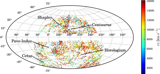
Distribution of 6dFGSv galaxies in Galactic latitude (l) and longitude (b), shown in an equal-area Aitoff projection. Individual galaxies are colour-coded by their redshift. The 6dFGSv galaxies fill the Southern hemisphere apart from ±10° about the Galactic plane. Some of the large-scale structures in the 6dFGSv volume are also indicated.
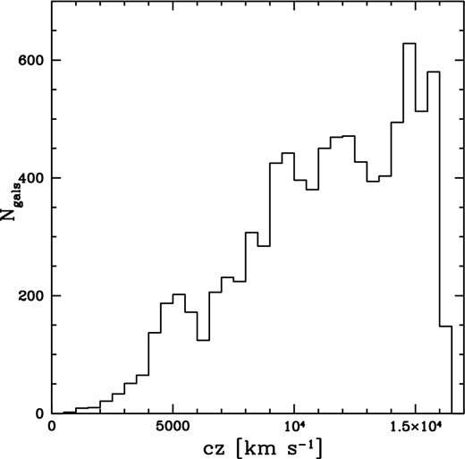
Redshift distribution of galaxies in 6dFGSv in the CMB reference frame. The bin width is 500 km s−1.
2.2 Reconstructed velocity fields
We wish to compare our observed velocity field to reconstructed velocity field models derived from the redshift-space distribution of galaxies, under the assumption that the matter distribution traces the galaxy distribution. We present here two different velocity field reconstructions, one derived from the 2MASS Redshift Survey (Erdoğdu et al. 2014), and one derived from the PSCz survey (Branchini et al. 1999). In a future paper, we will also compare the observed velocity field to other reconstructions, including the 2M++ reconstruction (Lavaux & Hudson 2011). This follows Carrick et al. (in preparation), who have made such a comparison between 2M++ and SFI++.
2.2.1 2MRS reconstructed velocity field
At present, one of the largest and most complete reconstructed velocity fields is derived from galaxies in the 2MASS Redshift Survey (2MRS). In the final data release (Huchra et al. 2012), the 2MRS consists of redshifts for 44 699 galaxies with a magnitude limit of Ks = 11.75 (with a significant fraction of the Southern hemisphere redshifts coming from 6dFGS). The zone of avoidance for the sample varies with Galactic longitude, but lies at roughly |b| ∼ 5 − 8°, and the sample covers 91 per cent of the sky. We thus make use of the 2MRS reconstructed density and velocity fields of Erdoğdu et al. (2014; updated from Erdoğdu et al. 2006) which uses the 2MRS redshift sample to recover the linear theory predictions for density and velocity.
The method of reconstruction is outlined in Erdoğdu et al. (2006), where it was applied to a smaller 2MRS sample of 20 860 galaxies with a brighter magnitude limit of Ks = 11.25 and a median redshift of 6000 km s−1. The method closely follows that of Fisher et al. (1995) and relies on the assumption that the matter distribution traces the galaxy distribution in 2MRS, with a bias parameter |$\beta = \Omega _{\rm m}^{0.55} / b$| that is assumed to take the value 0.4 for the 2MRS sample. The density field in redshift space is decomposed into spherical harmonics and Bessel functions (or Fourier–Bessel functions) and smoothed using a Wiener filter. The velocity field is derived from the Wiener-filtered density field by relating the harmonics of the gravity field to those of the density field (in linear theory). The reconstruction gives velocity vectors on a grid in supergalactic Cartesian coordinates with gridpoints spaced by 8 h−1 Mpc and extending to a distance of 200 h−1 Mpc from the origin in each direction. (h is the Hubble constant in units of 100 km s−1 Mpc−1.)
Erdoğdu et al. (2006) explore the issue of setting boundary conditions in the density and velocity field reconstruction. One must make some assumptions about the calibration of the reconstructed density field. The density/velocity field reconstruction used in this paper defines the logarithmic derivative of the gravitational potential to be continuous along the surface of the sphere of radius 200 h−1 Mpc. This is the ‘zero potential’ boundary condition, as described in the aforementioned papers. For a perfectly smooth, homogeneous universe, one would then expect that both the mean overdensity and mean peculiar velocity within the spherical survey volume would also be zero. However, because of the particular geometry of local large-scale structure, both of these quantities deviate slightly from zero. The mean overdensity within 200 h−1 Mpc is found to be δ = +0.09 (with an rms scatter of 1.21), and the mean line-of-sight velocity is found to be +66 km s−1(with an rms scatter of 266 km s−1). (Here, δ represents the local matter density contrast.) In contrast to what one might naively expect, the slightly positive mean value of δ induces a positive value to the mean line-of-sight peculiar velocity. This occurs because many of the largest structures lie at the periphery of the survey volume.
For comparison with our observed velocities, we convert the 2MRS velocity grid from real space to redshift space. Each real-space gridpoint is assigned to its corresponding position in redshift space, and resampled on to a regularly spaced grid in redshift space. The points on the redshift-space grid are 4 h−1 Mpc apart, and we have linearly interpolated the nearest points from the old grid on to the new grid to get the redshift-space velocities.
Because the real-space velocity field is Weiner-filtered on to a coarsely sampled grid with 8 h−1 Mpc spacing, there are no apparent triple-valued regions in the field. That is, there are no lines of sight along which the conversion from real space to redshift space becomes confused because a single redshift corresponds to three different distances, as can happen in the vicinity of a large overdensity. For triple-valued regions to appear in a grid with 8 h−1 Mpc spacing one would need velocity gradients as large as 800 km s−1 between adjacent points in the grid, and this does not occur anywhere in the velocity field. While the actual velocity field will presumably include such triple-valued regions around rich clusters, they have been smoothed out in this model.
2.2.2 PSCz reconstructed velocity field
An alternative reconstruction of the density and velocity fields is offered by Branchini et al. (1999), who make use of the IRAS Point Source Catalogue Redshift Survey (PSCz, Saunders et al. 2000). PSCz includes 15,500 galaxies, with 60 μm flux f60 > 0.6. The survey covers 84 per cent of the sky, with most of the missing sky area lying at low Galactic latitudes (see Branchini et al. 1999, fig. 1.) While the number of galaxies is far fewer than in 2MRS, Erdoğdu et al. (2006) show that the redshift histogram drops off far more slowly for PSCz than for 2MRS, so that the discrepancy in the number of objects is not as great at distances of ∼100–150 h−1 Mpc, where most of our 6dFGSv galaxies lie.
The density and velocity fields were reconstructed from PSCz by spherical harmonic expansion, based on a method proposed by Nusser & Davis (1994). The method uses the fact that, in linear theory, the velocity field in redshift space is irrotational, and so may be derived from a velocity potential. The potential is expanded in spherical harmonics, and the values of the spherical harmonic coefficients are then derived, again assuming a mapping between the PSCz galaxy redshift distribution and the matter distribution, with a bias parameter β = 0.5. The reconstruction gives velocity vectors on a supergalactic Cartesian grid with spacing 2.8 h−1 Mpc, extending to a distance of 180 h−1 Mpc from the origin in each direction. The mean overdensity within the survey volume is δ = −0.11 (with an rms scatter of 1.11), with a mean line-of-sight velocity of +79 km s−1(with an rms scatter of 156 km s−1).
We convert the PSCz velocity grid from real space to redshift space, using the same procedure used to construct the 2MRS velocity field. However, in this instance, the velocity grid uses the same 2.8 h−1 Mpc grid spacing that is used in the real-space field. While the original grid spacing is finer in the PSCz reconstruction than in the 2MRS reconstruction, Branchini et al. (1999) minimize the problem of triple-valued regions by collapsing galaxies within clusters, and applying a method devised by Yahil et al. (1991) to determine the locations of galaxies along those lines of sight.
2.2.3 Comparing the model density fields
The two model density fields are shown in Fig. 3. In the left column, along four different slices of SGZ, we show the reconstructed 2MRS density field. (SGX, SGY, and SGZ are the three cardinal directions of the supergalactic Cartesian coordinate system, with SGZ = 0 representing the supergalactic plane.) The field has been smoothed using a 3D Gaussian kernel, which we explain in greater detail in Section 5, when we apply this smoothing algorithm to the velocity field. In the central column, we show the smoothed PSCz field, and in the right column, we show the ratio of the 2MRS and PSCz densities. We only show gridpoints with distances out to 161.2 h−1 Mpc, the distance corresponding to the 6dFGSv limiting redshift of 16 120 km s−1.
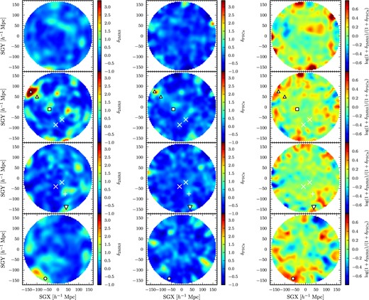
Gaussian smoothed versions of the 2MRS matter density field (left), the PSCz matter density field (centre) and the logarithm of the ratio between the 2MRS and PSCz densities (right) in four slices parallel to the supergalactic plane, covering the ranges (from top to bottom) SGZ>+20 h−1 Mpc, −20<SGZ<+20 h−1 Mpc, −70<SGZ<−20 h−1 Mpc and SGZ<−70 h−1 Mpc. Note that δ is the density contrast, while 1 + δ is the density in units of the mean density of the Universe. The slices are arranged so that there are roughly equal numbers of 6dFGSv galaxies in each. Major large-scale structures are labelled: the Cetus Supercluster (▽), the Eridanus Cluster (+), the Horologium-Reticulum Supercluster (◯), the Hydra-Centaurus Supercluster (▿), the four most overdense regions of the Sculptor Wall (×), and the two main overdensities of the Shapley Supercluster (▵). Only gridpoints for which the distance to the origin is less than 161.2 h−1 Mpc are displayed, so that the limiting distance shown here matches the limiting redshift of 6dFGSv.
In this figure, we also plot the positions of several individual Southern hemisphere superclusters, as identified in the 6dFGS redshift survey. Based on the features identified by Jones et al. (2009), which itself relies on superclusters identified by Fairall (1998) and Fairall & Woudt (2006), among others, we highlight the positions of the Cetus Supercluster, Eridanus Cluster, Sculptor Wall, Hydra-Centaurus Supercluster, Shapley Supercluster, and Horologium-Reticulum Supercluster. Note that we mark multiple overdensities for a single structure in two cases: We mark both of the two main overdensities of the Shapley Supercluster (as identified by Fairall 1998), and four overdensities of the Sculptor Wall. The figure is indicative only, since superclusters are extended objects and we have marked them as points. Nonetheless, the points marked on the figure provide a useful guide in the discussion in Section 5.1.2, in which we will compare the locations of these superclusters to the features of the observed and predicted velocity fields.
A few points that should be made in examining this comparison of the two models: (1) The Shapley Supercluster appears as the most prominent overdensity within ∼150 h−1 Mpc, particularly in the 2MRS model. (2) There is no one particular region of the sky that shows an unusually strong deviation between the two models. Rather, the deviations between the models are scattered across the sky, with the largest differences appearing on the outskirts of the survey volume. (3) The plot illustrates what was stated in the previous subsection: the scatter in densities (and velocities) is somewhat larger in the 2MRS model than the PSCz model, meaning that the former model includes more overdense superclusters and more underdense voids. This may suggest that the fiducial value of β that was assumed for the 2MRS model is too large, or that the fiducial value of β assumed for the PSCz model is too small. We explore that possibility in greater detail in a future paper (Magoulas et al. in preparation).
While Fig. 3 shows that the familiar features of large-scale structure are apparent in both models, we can also ask whether the two model density fields predict similar peculiar velocities on the scale of individual gridpoints. In Fig. 4, we show contour plots of 2MRS model velocities plotted against PSCz model velocities for all gridpoints out to 16 120 km s−1, the redshift limit of 6dFGSv. For nearby points (cz < 8000 km s−1) the velocities in the two models are, as expected, positively correlated with a slope close to unity. However at larger distances the correlation grows weaker, mainly because the number of galaxies is decreasing rapidly with redshift for both surveys (again, see the comparison in Erdoğdu et al. 2006). At redshifts of ∼12 000 km s−1or greater (where roughly half of our 6dFGSv galaxies lie), there is virtually no correlation between the velocities of the two models on the scale of individual grid points. This is because the PSCz survey in particular has very sparse sampling at these distances and so is heavily smoothed.
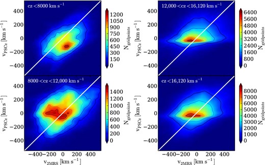
Contour plots, comparing the model velocities from 2MRS and PSCz, calculated at individual gridpoints for different redshift slices. The lower right panel shows all gridpoints with cz < 16, 120 km s−1, which is the redshift limit of 6dFGSv. The remaining three panels show subsets of this volume, with redshift ranges written at the top of each panel. The colour bars show the number of gridpoints found within a single smoothing length, which corresponds to 40 × 40 km s−1. The white diagonal line in each panel shows the 1-to-1 line. We note that while the velocities from the two models appear to be correlated at low redshift, that correlation fades way for the gridpoints at higher redshift (where we find the bulk of our 6dFGSv galaxies).
3 FITTING THE FUNDAMENTAL PLANE
3.1 Maximum likelihood methodology
We employ a maximum likelihood method to fit the FP, similar to the method developed by Colless et al. (2001) and Saglia et al. (2001) to fit the EFAR sample. The method is explained in detail in Magoulas et al. (2012), but summarized below.
As Colless et al. (2001) noted, when plotted in r-s-i space, early-type galaxies are well represented by a 3D Gaussian distribution. This was shown to be true for 6dFGS by Magoulas et al. (2012) (see e.g. fig. 9 from that paper). Our maximum likelihood method then involves fitting the distribution of galaxies in r-s-i space to a 3D Gaussian, where the shortest axis is orthogonal to the FP and characterizes the scatter about the plane, while the other two axes fit the distribution of galaxies within the plane.
We should also note that in previous papers, we investigated the possibility of adding one or more additional parameters to the FP fit. Magoulas et al. (2012) investigated FP trends with such parameters as environment and morphology. Springob et al. (2012) investigated the FP space trends with stellar population parameters. The only supplemental parameter with the potential to improve our FP fit was stellar age, as explained by Springob et al. (2012). However, as stated in that paper, while stellar age increases the scatter of the FP, the uncertainties on the measured ages of individual galaxies are too large to allow useful corrections for galaxy distances. We thus do not include any corrections for stellar age, or any other stellar population parameters, in the FP fitting done here.
3.2 Calibrating the FP zero-point
In the expression r = as + bi + c, the value of c gives us the zero-point, and the calibration of the relative sizes of the galaxies depends on how one determines the value of c. As we are using the FP to measure peculiar velocities, it also gives us the zero-point of peculiar velocities (or more specifically, the zero-point of logarithmic distances). We need to make some assumption about the peculiar velocity field, in order to set the zero-point of the relation. When we fit the FP in Magoulas et al. (2012), for example, we assumed that the average radial peculiar velocity of the galaxies is zero.
For a large all-sky sample, the assumption that the average peculiar velocity of the sample is zero is equivalent to assuming that the velocity field includes no monopole term, since a monopole (an error in the expansion rate given by H0) is completely degenerate with an offset in the FP zero-point. As long as the galaxies are evenly distributed across the whole sky, this assumption only impacts the velocity field monopole, and we can still measure higher order multipoles. The situation is somewhat different in the case of a sample that only includes galaxies in one hemisphere, however. In this case, assuming that the mean velocity of the galaxies in the sample is zero means suppressing the polar component of the dipole. In the case of a Southern hemisphere survey with a dipole motion directed along the polar axis, for example, assuming that the mean velocity of the galaxies is zero corresponds to calibrating out the entire dipole.
6dFGS is of course just such a hemispheric survey. We can essentially eliminate this FP calibration problem, however, if we set the zero-point using only galaxies close to the celestial equator. Such a ‘great circle’ sample is, like a full-sphere sample, only degenerate in the monopole – even if the velocity field includes a dipole with a large component along the polar direction, this component has negligible impact on the radial velocities of galaxies close to the celestial equator.
How do we then set the zero-point with such a great circle sample? Recall that the zero-point c is not represented by any of the eight parameters in our 3D Gaussian model alone. Rather, it is a function of multiple FP parameters (explicitly, |$c=\bar{r}-a \bar{s}-b \bar{i}$|). However, if we fix the other FP parameters to the fitted values for the entirety of the sample, then the zero-point is represented by |$\bar{r}$|. This is a quantity that we measured to be |$\bar{r}=0.184 \pm 0.005$| for the whole sample. However, because of degeneracies between |$\bar{r}$|, |$\bar{s}$|, |$\bar{i}$|, and the slopes a and b, 0.005 dex does not represent the true uncertainty in the zero-point.
We define our equatorial sample as the Ng = 3781 galaxies with −20° ≤ δ ≤ 0°, and fit the FP zero-point (|$\bar{r}$|) after fixing the other coefficients that define the FP (|$a,b,\bar{s},\bar{\imath },\sigma _1,\sigma _2, \sigma _3$|) to the best-fitting values from the full sample. The best-fitting value of the mean effective radius for the equatorial subsample is |$\bar{r}=0.178$|. For this equatorial sample, the uncertainty on |$\bar{r}$| would be 0.007 dex if we were fitting for all eight FP parameters. However, because we constrain all parameters except for |$\bar{r}$|, the uncertainty is only 0.003 dex, and this represents our uncertainty in the zero-point of the relation. This measurement of the uncertainty assumes a Gaussian distribution of peculiar velocities in the great circle region, with no spatial correlation.
Despite the fact that we have calibrated the zero-point of the FP relation using the galaxies in the range −20° ≤ δ ≤ 0°, to mitigate the possibility of a large dipole motion biasing the zero-point, we cannot rule out the possibility of a monopole in the velocity field within that volume creating such a bias. In Section 5.1.2, we explore the possibility of an offset in the zero-point of the FP relation in greater detail.
Finally, we note that there is the potential for some bias in the zero-point due to the fact that −20° ≤ δ ≤ 0° is not exactly a great circle. The extent of this bias depends on the size of the bulk flow's polar component relative to the mean velocity dispersion of galaxies. If we assume that the mean velocity dispersion of galaxies is ∼300 km s−1, then we estimate that a comparably large bulk flow of ∼300 km s−1along the celestial pole would introduce a bias of 0.0007 dex in the zero-point. This is much smaller than our 0.003 dex uncertainty, however, and a ∼300 km s−1bulk flow along the polar direction alone is most likely a pessimistically large estimate.
4 DERIVING PECULIAR VELOCITIES
4.1 Bayesian distance estimation
When measuring a galaxy distance, authors typically derive a single number, along with its error. If the distance estimates have a Gaussian distribution, these two numbers fully characterize the probability distribution for the galaxy distance. However, it is often more natural to estimate the logarithm of the distance, particularly if it is this quantity that has a Gaussian error distribution. This in fact applies to distance estimates using the FP, which is fit in logarithmic r-s-i space.
However, because of the various selection effects and bias corrections, the probability distribution is not exactly Gaussian in logarithmic distance. Thus in order to retain all the available information, we choose to calculate the full posterior probability distributions for the distance to each galaxy. This requires that we have a clear understanding of the definitions being used in the previous section.
We have referred to ‘Fundamental Plane space’, by which we mean the 3D parameter space defined by r, s and i. r, s and i can be described either as observational parameters or physical parameters. That is, galaxy radius, velocity dispersion, and surface brightness are all clearly observational parameters, but they are also (when defined appropriately) physical properties that the galaxy possesses independent of any particular set of observations. When we fit the FP we are simultaneously fitting an empirical scaling relation of observable quantities for our particular sample and deriving a scaling relation of physical quantities that should hold for any similarly selected sample.
How then do we calculate the probability distribution for distance? Because equation (5) provides the probability distribution of physical radius for given values of velocity dispersion and surface brightness, the simplest approach available to us is to calculate P(Δrn|rz, n, sn, in) over an appropriate range of Δr values, and then use a transformation of variables to get P(Δdn|rz, n, sn, in). P(Δrn|rz, n, sn, in) is the posterior probability that the ratio of the nth galaxy's size at its redshift distance to its size at its true comoving distance (in logarithmic units) is Δrn. P(Δdn|rz, n, sn, in) is the corresponding posterior probability for the ratio of comoving distances for galaxy n. Since the redshift of the galaxy is given and dz is known, P(Δdn|rz, n, sn, in) is equivalent to P(dH, n|rz, n, sn, in).
We implement this approach in the following manner.
Specify the FP template relation using our fitted 3D Gaussian model, as described by the eight parameters a, b, |$\bar{r}$|, |$\bar{s}$|, |$\bar{\imath }$|, σ1, σ2, and σ3. The best-fitting values of these parameters are given in Magoulas et al. (2012) for various samples and passbands. For the full J-band sample that we are using here, the best-fitting values are: a = 1.438, b = −0.887, |$\bar{r}=0.178$|, |$\bar{s}=2.187$|, |$\bar{\imath }=3.175$|, σ1 = 0.047, σ2 = 0.315, and σ3 = 0.177. The value of |$\bar{r}$| was specifically fit to the region −20° ≤ δ ≤ 0°, as explained in Section 3.2.
For each individual galaxy n, loop through every possible logarithmic comoving distance dH, n that the galaxy could have. Distance is of course a continuous quantity, but in practice we are limited to examining a finite number of possible distances. We consider 501 evenly spaced values of Δdn, between −1.0 and +1.0 in steps of 0.004 dex, and compute the corresponding values of Δrn. These steps correspond to 1 per cent in relative distance.
- For each of these possible logarithmic ratios of radius, use Bayes’ theorem to obtain the posterior distribution for the nth galaxy's size as a function of the observables,Given our assumed physical radius rH, n, we can evaluate |$P({{\boldsymbol x}_{n}})$| in equation (5), on the assumption that |$P({{\boldsymbol x}_{n}}) = P(r_{z,n},s_n,i_n|\Delta r_{n})$|, so long as the |${{\boldsymbol x}_{n}}$| in question uses the physical radius corresponding to the distance dH, n. That is, while equation (5) is written in such a way that it suggests that there is a single probability density |$P({{\boldsymbol x}_n})$| for galaxy n, we now suggest that for galaxy n, we must consider many possible distances that the galaxy could be at, each of which corresponds to a different radius and different |${{\boldsymbol x}_n}$|.(13)\begin{equation} P(\Delta r_{n}|r_{z,n},s_n,i_n) = {P(r_{z,n},s_n,i_n|\Delta r_{n}) P(\Delta r_{n}) \over P(r_{z,n},s_n,i_n)}. \end{equation}
Having evaluated P(rz, n, sn, in|Δrn), we multiply by the prior, P(Δrn), assumed to be flat, and apply the proper normalization (that is, normalizing the probabilities so that the total probability across all possible radii is unity), to give us the posterior probability P(Δrn|rz, n, sn, in).
- Convert the posterior probability distribution of sizes, P(Δrn|rz, n, sn, in), to that of distances, P(Δdn|rz, n, sn, in), by changing variables from r to d. To do so, we use the fact that(14)\begin{equation} P(\Delta d_{n}) = P(\Delta r_{n}) {d[\Delta r_{n}] \over d[\Delta d_{n}]}. \end{equation}
The question of how to calculate the different normalization terms fn in equation (5) is addressed in the following subsection. However, it should be noted that whether one needs to include this term at all depends on what precisely the probability distribution in question is meant to represent. If we were interested in the probability distribution of possible distances for each individual galaxy considered in isolation, then the fn term should be omitted. In this case, however, we are computing the probability distribution of the comoving distance corresponding to the redshift-space position of galaxy n, and so the fn term must be included.
4.2 Selection bias
Malmquist bias is the term used to describe biases originating from the spatial distribution of objects (Malmquist 1924). It results from the coupling between the random distance errors and the apparent density distribution along the line of sight. There are two types of distance errors that one must consider. The first of these is inhomogeneous Malmquist bias, which arises from local density variations due to large-scale structure along the line of sight. It is most pronounced when one is measuring galaxy distances in real space. This is because the large distance errors cause one to observe galaxies scattering away from overdense regions, creating artificially inflated measurements of infall on to large structures. By contrast, when the measurement is done in redshift space, the much smaller redshift errors mean that this effect tends to be negligible (see e.g. Strauss & Willick 1995).
For the 6dFGSv velocity field as presented in this paper, we are measuring galaxy distances and peculiar velocities in redshift space rather than real space. In this case, inhomogeneous Malmquist bias is negligible, and the form of Malmquist bias that we must deal with is of the second type, known as homogeneous Malmquist bias, which affects all galaxies independently of their position on the sky. It is a consequence of both (1) the volume effect, which means that more volume is covered within a given solid angle at larger distances than at smaller distances, and (2) the selection effects, which cause galaxies of different luminosities, radii, velocity dispersions etc., to be observed with varying levels of completeness at different distances. We note, however, that different authors use somewhat different terminology, and the latter effect described above is often simply described as ‘selection bias’.
The approach one takes in correcting for this bias depends in part on the selection effects of the survey. If the selection effects are not well defined analytically, then the bias correction can be complicated, though still possible. For example, Freudling et al. (1995) use Monte Carlo simulations to correct for Malmquist bias in the SFI sample (Giovanelli et al. 1994; Giovanelli et al. 1995).
In our case, however, we have explicit analytical expressions for the intrinsic distribution of physical parameters, and explicit and well-defined selection criteria. It is thus possible, at least in principle, to correct for selection bias analytically. However, as we will see, in practice we are obliged to use mock samples for the purposes of evaluating the relevant integral.
Our bias correction involves applying an appropriate weighting to each possible distance that the galaxy could be at in order to account for galaxies at those distances that are not included in our sample due to our selection criteria. One complication is that certain regions of FP space are not observed in our sample because of our source selection. The expression for the likelihood that we give in equation (5) includes a normalization factor fn that ensures the integral of |$P({{\boldsymbol x}_{n}})$| over all of FP space remains unity, even when certain regions of FP space are excluded by selection cuts.
We next consider what happens when, in addition to the s cut, we also have an apparent magnitude cut. At a particular logarithmic distance d, this corresponds to a cut in absolute magnitude, Mcut(d). At that distance, we observe all galaxies with s greater than scut and M brighter than Mcut(d), whereas we miss all others. A cut in absolute magnitude corresponds to a diagonal cut in r-s-i space, since absolute magnitude is a function of both r and i. We can incorporate this cut into the equation for fn by integrating i from −∞ to ∞, but r from rcut(i) to ∞, where rcut(i) is the radius at the surface brightness i corresponding to Mcut.
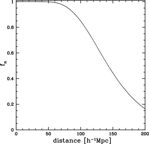
The normalization factor used to correct selection bias as a function of distance, derived from a mock sample with 100 000 galaxies.
Note that each galaxy has its own individual error matrix, En, and we should be using the specific En matrix for galaxy n. However, running such an Ng = 105 Monte Carlo simulation separately for all ∼9000 galaxies is computationally impractical. As a compromise, when we run the Monte Carlo simulation, we assign measurement errors to every mock galaxy parameter according to the same algorithm specified for 6dFGS mock catalogues explained in Magoulas et al. (2012) section 4. This treats the mock galaxy measurement errors as a function of apparent magnitude.
4.3 Peculiar velocity probability distributions
In Fig. 6 we show the posterior probability density distributions as functions of logarithmic distance for 10 randomly chosen 6dFGSv galaxies.
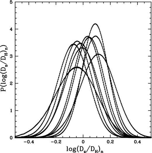
For 10 randomly chosen galaxies in 6dFGSv, we show the probability density distribution of Δdn = log (Dz/DH)n, which is the logarithm of the ratio of the comoving distance associated with galaxy n's redshift to the true comoving distance of the galaxy. The exact probability distributions are represented by circles, whereas the approximations from equation (21) are represented by solid lines.
The values of 〈Δd〉, ϵd, and α are given in Table 1. The interested reader can reconstruct the probability distributions from equation (21). However, note that this is an approximation, which breaks down in the wings of the distribution, as it can yield (physically impossible) negative values when the function approaches zero. The reconstructed probability distributions from equation (21) for the 10 galaxies shown in Fig. 6 are represented in that figure by solid lines.
6dFGSv logarithmic distance ratios, and associated parameters. The columns are as follows: (1) source name in 6dFGS catalogue; (2, 3) right ascension and declination (J2000); (4) individual galaxy redshift in the CMB reference frame; (5) group redshift in the CMB reference frame, in cases where the galaxy is in a group (set to −1 for galaxies not in groups); (6) group identification number (set to −1 for galaxies not in groups); (7) the logarithmic distance ratio 〈Δd〉 = 〈log (Dz/DH)〉; (8) the error on the logarithmic distance ratio, ϵd, derived by fitting a Gaussian function to the Δd probability distribution; (9) the skew in the fit of the Gaussian function, α, calculated using equation (22). The full version of this table is available in the electronic version of the journal.
| 6dFGS name | R.A. | Dec. | czgal | czgroup | Group number | 〈Δd〉 | ϵd | α |
|---|---|---|---|---|---|---|---|---|
| (deg.) | (deg.) | ( km s−1) | ( km s−1) | (dex) | (dex) | |||
| (1) | (2) | (3) | (4) | (5) | (6) | (7) | (8) | (9) |
| g0000144-765225 | 0.05985 | −76.8736 | 15941 | −1 | −1 | +0.1039 | 0.1296 | −0.0200 |
| g0000222-013746 | 0.09225 | −1.6295 | 11123 | −1 | −1 | +0.0870 | 0.0954 | −0.0066 |
| g0000235-065610 | 0.09780 | −6.9362 | 10920 | −1 | −1 | +0.0282 | 0.1073 | −0.0116 |
| g0000251-260240 | 0.10455 | −26.0445 | 14926 | −1 | −1 | +0.0871 | 0.1065 | −0.0111 |
| g0000356-014547 | 0.14850 | −1.7632 | 6956 | −1 | −1 | −0.0743 | 0.1165 | −0.0112 |
| g0000358-403432 | 0.14895 | −40.5756 | 14746 | −1 | −1 | −0.0560 | 0.1532 | −0.0217 |
| g0000428-721715 | 0.17835 | −72.2874 | 10366 | −1 | −1 | −0.0486 | 0.1123 | −0.0135 |
| g0000459-815803 | 0.19125 | −81.9674 | 12646 | −1 | −1 | −0.0131 | 0.1201 | −0.0153 |
| g0000523-355037 | 0.21810 | −35.8437 | 15324 | 14646 | 1261 | −0.0219 | 0.1145 | −0.0083 |
| g0000532-355911 | 0.22155 | −35.9863 | 14725 | 14646 | 1261 | +0.0421 | 0.1077 | −0.0098 |
Note that while we use the group redshift for galaxies found in groups, we provide here the individual galaxy redshifts in Table 1 as well. As explained in Section 2.1, we refer the interested reader to Magoulas et al. (2012) for a more detailed description of the grouping algorithm.
In Fig. 7, we show the histogram of the probability-weighted mean values of the logarithm of the ratio of redshift distance to Hubble distance Δdn for each of the 8885 galaxies in the 6dFGSv sample; put another way, this is the histogram of expectation values 〈Δdn〉. The mean of this distribution is +0.005 dex, meaning that we find that the peculiar velocities in the survey volume are very slightly biased towards positive values. The rms scatter is 0.112 dex, which corresponds to an rms distance error of 26 per cent. As explained in Magoulas et al. (2012), one might naively assume that the 29 per cent scatter about the FP along the r-axis translates into a 29 per cent distance error, but this neglects the fact that the 3D Gaussian distribution of galaxies in FP space is not maximized on the FP itself at fixed s and i. The distance error calculated by Magoulas et al. (2012) neglecting selection bias is 23 per cent, but the bias correction increases the scatter to 26 per cent.
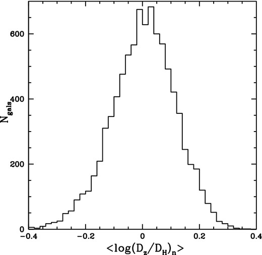
Distribution of 〈Δdn〉 = 〈log (Dz/DH)n〉, the expectation values of the logarithm of the ratio of redshift distance to Hubble distance Δdn for each of the 8885 galaxies in the 6dFGSv sample.
We note that while all of our analysis is conducted in logarithmic distance units, some applications of the data may require conversion to linear peculiar velocities. The interested reader is invited to convert these logarithmic distance ratios accordingly, accounting for the fact that the measurement errors are lognormal in peculiar velocity units. Further elaboration on this point is provided in Appendix A.
5 PECULIAR VELOCITY FIELD COSMOGRAPHY
In a future paper we will perform a power spectrum analysis on the peculiar velocity field in order to extract the full statistical information encoded in the linear velocity field. In this paper, however, we display the data in such a way as to illuminate these correlations, and to give us a cosmographic view of the velocity field. We approach this goal using adaptive kernel smoothing.
We impose a 3D redshift-space grid in supergalactic Cartesian coordinates, with gridpoints 4 h−1 Mpc apart. At each gridpoint we compute adaptively smoothed velocities from both the 2MRS predicted field and the 6dFGSv observed field using the following procedure. It draws on methods used by Silverman (1986) and Ebeling, White & Rangarajan (2006), but we have adjusted these approaches slightly to produce smoothing kernels that, on average, lie in the range ∼ 5–10 h−1 Mpc, as that appears to highlight the features of the velocity field around known features of large-scale structure most effectively.
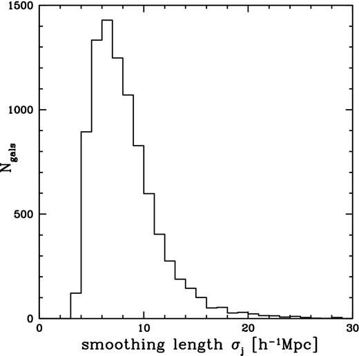
Distribution of smoothing lengths, σj, for all 6dFGSv galaxies, following equation (24).
5.1 Features of the velocity field
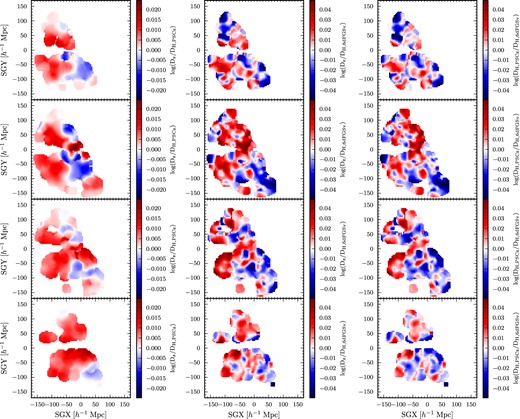
In Figs 9 and 10, we show the reconstructed 2MRS and PSCz velocity fields alongside the 6dFGS observed field. In each case, the velocity field has been smoothed, using the adaptive kernel smoothing described above. In Fig. 9, the four panels on the left column show the smoothed velocity field predicted by 2MRS, in slices of SGZ. The four panels in the central column show the observed 6dFGS velocity field, smoothed in the same manner. The four panels in the right column show the difference between the 2MRS velocity field and the 6dFGS velocity field. Fig. 10 follows the same format, but with the PSCz field in place of 2MRS. That is, the left column corresponds to the velocity field predicted by PSCz, and the right column corresponds to the difference between the PSCz field and the 6dFGS field. In each case the colour-coding gives the mean smoothed logarithmic distance ratio averaged over SGZ at each (SGX,SGY) position. We note that while Fig. 4 showed that the correlation between the 2MRS and PSCz model velocities weakens at higher redshifts, we see in Figs 9 and 10 that both models make qualitatively similar predictions for the velocity field on large scales.
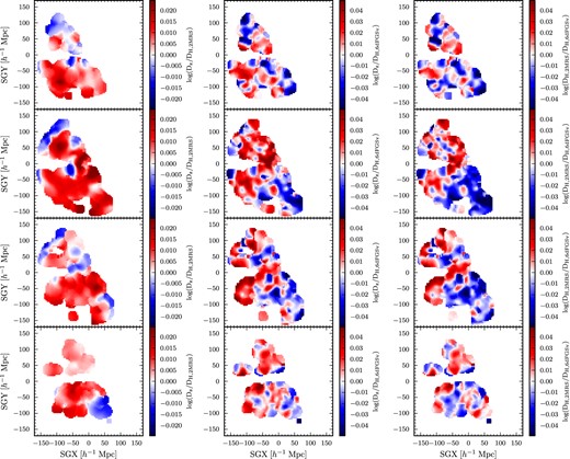
Adaptively smoothed versions of the reconstructed 2MRS velocity field, as derived by Erdoğdu et al. (2014) (left), the observed 6dFGS velocity field (centre) and the observed 6dFGS field minus the 2MRS reconstruction (right), in the same four slices of SGZ that are displayed in Fig. 3. In each case, the velocity field is given in logarithmic distance units (Δd = log (Dz/DH), in the nomenclature of Section 4.1), as the logarithm of the ratio between the redshift distance and the true Hubble distance. As shown in the colour bars for each panel, redder (bluer) colours correspond to more positive (negative) values of Δd, and thus more positive (negative) peculiar velocities. Gridpoints are spaced 4 h−1 Mpc apart.
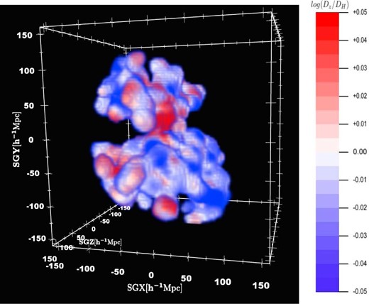
The smoothed 6dFGSv peculiar velocity field in 3D, plotted on a grid in supergalactic Cartesian coordinates, with gridpoints colour-coded by the value of Δd = log (Dz/DH). Adobe Reader version 8.0 or higher enables interactive 3D views of the plot, allowing rotation and zoom.
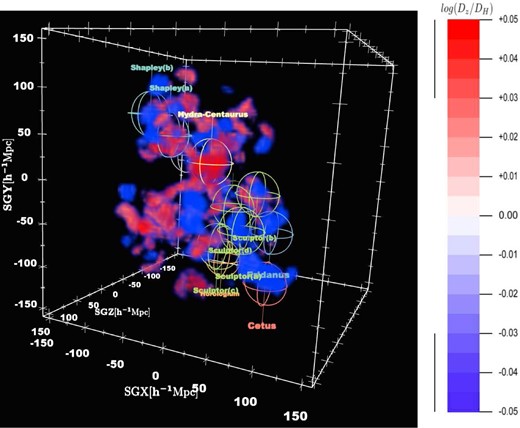
Same as Fig. 11, except that we only show gridpoints with Δd = log (Dz/DH) either greater than +0.03 or less than −0.03, in order to highlight the regions with the most extreme values. We also label each of the features of large-scale structure labelled in Fig. 3. Though they are outside the survey volume, we include labels for the Vela and Horologium-Reticulum superclusters, as they exert influence on the local velocity field. To toggle the visibility of individual superclusters in the interactive figure (Adobe Reader), open the Model Tree, expand the root model, and select the required supercluster name.
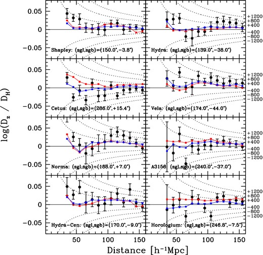
Averaged Δd = log (Dz/DH) for 6dFGS observations, as compared to both the 2MRS and PSCz models, in redshift-space distance bins along the Shapley Supercluster, Cetus Supercluster, Norma Cluster, Hydra-Centaurus Supercluster, Hydra Cluster, Vela Supercluster, Abell 3158, and Horologium-Reticulum Supercluster directions. Each bin is 10 h−1 Mpc wide, and the directions are defined as the regions within 30° of the coordinates listed at the bottom of each panel. For each bin, we have averaged the values of Δd for all 6dFGSv galaxies within the bin, and display the averaged value as the black circle. The error bar is then given by equation (27). The averaged Δd values as given by the 2MRS and PSCz models are represented by the red and blue squares, respectively. Red and blue lines connect the points. We also draw a black line at Δd = 0, and dotted lines to show the Δd values corresponding to ±400, 800, and 1200 km s−1, as indicated along the right-hand side of the plot.
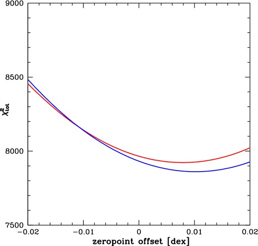
|$\chi _{\rm tot}^2$| as a function of the zero-point offset for 2MRS (red) and PSCz (blue). The best-fitting zero-point offsets are +0.0080 and +0.0102 dex for 2MRS and PSCz, respectively. These mean that the values of Δd would be shifted correspondingly lower in each case.
In addition to displaying the velocity fields in SGZ slices as in Figs 9 and 10, we would also like to view the fields in a fully 3D manner. Fig. 111 shows the smoothed 3D 6dFGSv peculiar velocity field.
We note that because of the adaptive smoothing, the mean error on the Δd value for a given gridpoint is relatively uniform across the survey volume. We find that the mean error, averaged over all gridpoints, is 0.02 dex in the 3D grid. However, because Figs 9 and 10 involve additional averaging of gridpoints, in that we collapse the grid on to four SGZ slices, the mean Δd error in those plots is 0.009. Thus features in that plot that vary by less than ∼0.009 may simply be products of measurement uncertainties.
5.1.1 Velocity field ‘monopole’
One must be careful in defining the terminology of the velocity moments when considering an asymmetric survey volume, such as the hemispheric volume observed by 6dFGS. In general, the zeroth order moment of the velocity field, or ‘monopole’, cannot be measured by galaxy peculiar velocity surveys. This is because the calibration of the velocity field usually involves an assumption about the zero-point of the distance indicator which is degenerate with a monopole term. The same logic applies to velocity field reconstructions, such as the 2MRS and PSCz reconstructions used in this paper.
In Section 2.2, we noted that the mean peculiar velocity of gridpoints in the 2MRS reconstruction is +66 km s−1. This value is of course dependent on the fact that we have assumed that the average gravitational potential is zero along the surface of a sphere of radius 200 h−1 Mpc. We now note that for the particular set of gridpoints located at the redshift-space positions of galaxies in our sample, the mean is actually somewhat more positive: +161 km s−1, with an rms of 297 km s−1. When converted into the logarithmic units of Δd and smoothed on to the 3D grid shown in Fig. 9, we find a mean value of 〈Δd〉 = +0.007 dex for the smoothed 2MRS gridpoints. This is close to the mean value of 〈Δd〉 = +0.005 found in the smoothed 6dFGS gridpoints. Similarly, for PSCz, the mean peculiar velocity of all gridpoints is +79 km s−1, while the mean at the positions of our 6dFGS galaxies is +135 km s−1, with an rms of 172 km s−1. This corresponds to 〈Δd〉 = +0.005. That is, in both the 2MRS and PSCz predictions and in the 6dFGS observations, we find that the mean peculiar velocities at the redshift-space positions of the galaxies in our sample skew somewhat towards positive values.
This is not, however, indicative of a monopole in the velocity field, as our survey only covers the Southern hemisphere. Rather, it is an indication that the model predicts a net positive mean motion of galaxies in the Southern hemisphere, at least within the hemisphere of radius ∼160 h−1 Mpc covered by the survey, and that our observations show a similarly positive mean motion of galaxies in the same hemispheric volume. (And, of course, the latter result depends on the assumption that the mean logarithmic comoving distance ratio, 〈Δd〉, is zero along a great circle in the celestial equatorial region.)
While the mean value of 〈Δd〉 is the same for both the predicted and observed fields, the standard deviation is not. As noted in Section 4.3, the scatter in 〈Δd〉 for the 6dFGSv galaxies is 0.112 dex. With the adaptive kernel smoothing, this scatter is reduced to 0.023 dex, whereas for the smoothed 2MRS and PSCz predicted fields, the scatter is only 0.009 and 0.007 dex, respectively. So, while the three fields have the same mean value for 〈Δd〉, the 〈Δd〉 values in the predicted field have a scatter which is comparable to their mean offset from zero, resulting in very few points with negative values. The scatter is much larger in the observed field, resulting in many more gridpoints with negative values.
The offset of 〈Δd〉 from zero then does not necessarily indicate the existence of a velocity field monopole, but may simply reflect the existence of higher order moments such as the dipole, with net positive motion towards the Southern hemisphere. We consider the velocity field dipole in the context of the origin of the bulk flow in the following subsection.
5.1.2 Velocity field dipole and comparison with models
Measurements of the peculiar velocity field dipole, or ‘bulk flow’, have been a source of some controversy in recent years. Despite differences in the size and sky distribution of the various peculiar velocity catalogues, there is general agreement among authors on the direction of the bulk flow in the local universe. For example, Watkins et al. (2009), Nusser & Davis (2011), and Turnbull et al. (2012), among others, all find a bulk flow whose direction, in supergalactic coordinates, points towards sgl ∼ 160°, sgb ∼ −30°, roughly between the Shapley Supercluster and the Zone of Avoidance.
Disagreement remains, however, about the magnitude of the bulk flow, and the extent to which the value may be so large as to represent a disagreement with the standard model of ΛCDM cosmology. Watkins et al. (2009), for example, claim a bulk flow of ∼400 km s−1on a scale of 50 h−1 Mpc, which is larger than predicted by the standard ΛCDM parameters of Wilkinson Microwave Anisotropy Probe (WMAP) (Hinshaw et al. 2013) and Planck (Planck Collaboration et al. 2013a). Others, such as Nusser & Davis (2011), claim a smaller value that is not in conflict with the standard model.
If the bulk flow is larger than the standard cosmology predicts, then it may be because the standard cosmological picture is incomplete. In a ‘tilted universe’ (Turner 1991), for example, some fraction of the CMB dipole is due to fluctuations from the pre-inflationary Universe. In that case, we would expect to observe a bulk flow that extends to arbitrarily large distances. (Though it should be noted that the results of Planck Collaboration et al. 2013b cast the plausibility of the titled universe scenario into doubt.)
However, a large bulk flow could instead have a ‘cosmographic’ rather than a ‘cosmological’ explanation. The geometry of large-scale structure near the Local Group may be such that it induces a bulk flow that is much larger than would typically be seen by a randomly located observer. In particular, there has been debate regarding the mass overdensity represented by the Shapley Supercluster (e.g. Hudson 2003; Proust et al. 2006; Lavaux & Hudson 2011), which, as seen in Fig. 3, represents the most massive structure within ∼150 h−1 Mpc. (We should note, however, that the dichotomy between a cosmological and cosmographic explanation for a large bulk flow expressed above is somewhat incomplete. A cosmographic explanation could have its own cosmological origins, in that a deviation from ΛCDM could impact the local cosmography. Nonetheless, certain cosmological origins for the bulk flow, such as a tilted universe, would not necessarily have such an impact on the cosmography.)
Whether we are able to identify the particular structures responsible for the bulk flow thus bears on what the origin of the large bulk flow might be. Most previous data sets were shallower than 6dFGSv, so this is of particular interest in this case. Our survey volume covers most of the Shapley Supercluster, allowing us to compare the predicted and observed velocities in the Shapley region. In Magoulas et al. (in preparation) and Scrimgeour et al. (in preparation), we will make quantitative measurements of both the bulk flow and the ‘residual bulk flow’ (the component of the velocity dipole not predicted by the model velocity field), but those results will be informed by our cosmographic comparison here.
Rather than simply compute a global |$\chi ^2_{\nu }$|, we can also investigate the agreement between data and model along particular lines of sight. Note that most of the Southern hemisphere structures highlighted in Fig. 3 lie roughly along two lines of sight, ∼130° apart. Hereafter, we refer to these directions as the ‘Shapley direction’ (the conical volume within 30° of (sgl, sgb) = (150|${^{\circ}_{.}}$|0, −3|${^{\circ}_{.}}$|8)) and the ‘Cetus direction’ (the conical volume within 30° of (sgl, sgb) = (286|${^{\circ}_{.}}$|0, +15|${^{\circ}_{.}}$|4)). These sky directions correspond to the positions of the more distant concentration of the Shapley Supercluster and the Cetus Supercluster, as identified in Fig. 3, respectively.
We can see the velocity flows along both of these directions in 3D in Fig. 11. However, even with such an interactive plot, one cannot easily see deep into the interior of the survey volume. To mitigate this problem, we have created Fig. 12, which is identical to Fig. 11, except that only certain gridpoints are highlighted. In this figure, we display only those gridpoints with extreme values of Δd (greater than +0.03 or less than −0.03 dex). We also highlight the positions of each of the superclusters highlighted in Fig. 3, in addition to the position of the Vela Supercluster (see below).
As seen in these figures, we find mostly positive peculiar velocities along the Shapley direction, and negative peculiar velocities along the Cetus direction. Does this agree with the models? In the Shapley direction alone, |$\chi ^2_{\nu }=0.920$| for 2MRS and 0.917 for PSCz. Whereas in the Cetus direction alone, |$\chi ^2_{\nu }=0.914$| for 2MRS and 0.898 for PSCz. Thus the agreement between data and models is somewhat worse along each of these lines of sight than it is in the survey volume as a whole.
As a point of comparison, we have generated similar plots for several additional lines of sight, shown in the remaining panels in Fig. 13. We show the binned Δd values along the directions of the Norma Cluster, the Hydra-Centaurus Supercluster, the Hydra Cluster, and the Vela Supercluster. The first three structures are familiar features of the local large-scale structure, noted by numerous past authors (e.g. LB88; Tully et al. 1992; Mutabazi et al. 2014). Vela is less well know, but Kraan-Korteweg et al. (in preparation) find preliminary observational evidence for a massive overdensity in that direction at cz ∼ 18 000–20 000 km s−1. Each of these four sky directions lies closer to the Shapley direction than the Cetus direction. They also lie close to both the Zone of Avoidance and the bulk flow directions observed by various authors, such as Feldman et al. (2010), Nusser & Davis (2011), and Turnbull et al. (2012). Additionally, they each show a similar trend to the one seen in the Shapley direction: the Δd values lie above the model predictions from both 2MRS and PSCz.
The remaining two panels in Fig. 13 show the velocity field along the directions towards Abell 3158 and the Horologium-Reticulum Supercluster. These are much closer to the Cetus direction than the Shapley direction, and they show a similar trend to the one seen for Cetus: Δd values which lie below the model predictions from both 2MRS and PSCz. Like Cetus, they also show a somewhat larger divergence between the 2MRS and PSCz model predictions, with PSCz lying closer to our observed Δd values.
These plots confirm what can be seen in Figs 9 and 10 as well. There is a gradient of residuals from the model, going from somewhat negative residuals in the Cetus direction, to more positive residuals in the Shapley direction, with the Cetus direction representing a particularly large deviation between the data and model for 2MRS, at least in terms of the mean value of Δd, even if the |$\chi ^2_{\nu }$| value in that region is no worse than the corresponding value in the Shapley direction. This suggests a residual bulk flow from both the 2MRS and PSCz models, pointing in the vicinity of the Shapley Supercluster, which is explored in greater detail by Magoulas et al. (in preparation).
One might worry that the apparent direction of this residual bulk flow lies close to the Galactic plane. Might erroneous extinction corrections be creating a systematic bias, which skews our results? As noted in Section 2.1, a previous iteration of this catalogue made use of the Schlegel et al. (1998) extinction map rather than the Schlafly & Finkbeiner (2011) extinction map. We find virtually no change in the cosmography, when using the Schlegel et al. (1998) corrections rather than those of Schlafly & Finkbeiner (2011). Magoulas et al. (in preparation) investigates this issue further, measuring the bulk flow when the extinction corrections are changed by as much as three times the difference between the Schlegel et al. (1998) and Schlafly & Finkbeiner (2011) corrections, finding only small changes in both the magnitude and direction of the bulk flow between one extreme and the other. It thus seems unlikely that the apparent residual bulk flow is an artefact of erroneous extinction corrections, unless the Schlafly & Finkbeiner (2011) extinction map includes systematic errors across the sky far larger than the difference between those values and those of Schlegel et al. (1998).
So, in summary, the global |$\chi ^2_{\nu }$| is ∼1 for both models, though lower for PSCz than for 2MRS. Both models systematically predict peculiar velocities that are too negative in the Shapley direction, and too positive in the Cetus direction. This suggests a ‘residual bulk flow’ that is not predicted by the models.
The residual bulk flow suggests that either the models may be underestimating features of large-scale structure within the survey volumes of both 2MRS and PSCz, or the velocity field is being influenced by structures outside the survey volume. However, the fact that the larger discrepancy in mean Δd occurs in the Cetus direction rather than the Shapley direction would seem to argue against a more-massive-than-expected Shapley Supercluster being the main cause of the residual bulk flow, unless we are underestimating the zero-point of the FP by much more than the 0.003 dex uncertainty derived in Section 3.2.
We did note in Section 3.2, however, that the calibration of the FP zero-point depends on the assumption that the sample of galaxies within the equatorial region (those galaxies in the range −20° < decl. < 0°) exhibit no monopole feature in the velocity field. We could ask, at this point, whether shifting the zero-point might change the agreement between data and model.
We thus calculate |$\chi ^2_{\rm tot}$| for both the 2MRS and PSCz models, allowing the zero-point of Δd to vary as a free parameter. As seen in Fig. 14, the best-fitting zero-point for 2MRS and PSCz, respectively, would be +0.0080 and +0.0102 dex higher than our nominal value. This ‘higher zero-point’ means that the Δd values would be correspondingly lower (i.e. the redshift distance is less than the Hubble distance). Thus, allowing the zero-point to float as a free parameter in the comparison to both 2MRS and PSCz models would have the effect of improving the overall fit, but making the offset in the mean value of Δd between data and models in the Cetus direction worse.
Finally, is there anything that we can say about the differences between the two velocity field models, and why PSCz offers a better fit to the 6dFGSv velocities than 2MRS does? To see why the 2MRS and PSCz velocity fields differ, it is instructive to look at the respective density fields, as shown in Fig. 3.
As seen in that figure, while the same basic features of large-scale structure appear in both models, they differ in the details, with a mean rms of the log density ratio on a gridpoint-by-gridpoint basis being 0.73 dex. (The scatter appears somewhat smaller than this in Fig. 3, because we have averaged gridpoints at a given SGX, SGY position on to our four SGZ slices.) The deviations are greatest at the edges of the survey volume, though relatively evenly spread across the sky, with no one particular feature of large-scale structure dominating the differences between the models. Within 161 h−1 Mpc, the mean overdensity 〈δ〉 is −0.07 in 2MRS and −0.15 in PSCz. With PSCz being, on average, less dense than 2MRS near the limits of the 6dFGS survey volume, it features more negative peculiar velocities in both the Shapley and Cetus directions, perhaps accounting for some of the better agreement with 6dFGSv in the Cetus direction.
We should note that, as seen in the original 2MRS and PSCz papers (Erdoğdu et al. 2006; Branchini et al. 1999), both surveys have very few galaxies at redshifts of cz ∼ 15 000 km s−1and greater, leading to considerable uncertainty in the density/velocity model at those redshifts. A future paper will improve on this limitation by comparing the observed velocity field to the deeper 2M++ reconstruction (Lavaux & Hudson 2011). In the future, deeper all-sky redshift surveys, such as WALLABY (Duffy et al. 2012) and TAIPAN (Beutler et al. 2011; Colless, Beutler & Blake 2013), should be able to provide more accurate models of both the density and velocity fields at the distance of structures such as Shapley. Those same surveys will also provide significantly more peculiar velocities than are presently available, which may be enough to resolve the source of any residual discrepancies between data and models.
6 CONCLUSIONS
We have derived peculiar velocity probability distributions for 8885 galaxies from the peculiar velocity subsample of the 6dFGS. We have presented a Bayesian method for deriving the probability distributions, which are nearly Gaussian with logarithmic distance. The Bayesian approach allows us to take advantage of the full probability distribution, accounting for the fact that it is not perfectly Gaussian in logarithmic units (and certainly not in linear units). In the units of the logarithmic distance ratio, Δd, we find a mean value of Δd equal to +0.005, in agreement with the slightly positive values for Southern hemisphere galaxies given by the 2MRS and PSCz models. The mean scatter in Δd for individual galaxies is 0.112 dex, corresponding to a 26 per cent distance error in linear units.
The peculiar velocities are then smoothed using an adaptive Gaussian kernel to give 3D maps of the observed velocity field. We similarly smooth the 2MRS and PSCz predicted velocity fields, and compare them to the 6dFGSv field. We find |$\chi _{\nu }^2=0.897$| for 2MRS and |$\chi _{\nu }^2=0.893$| for PSCz. The difference in total χ2 is 36, favouring the PSCz model with high significance. Though |$\chi _{\nu }^2 \sim 1$| in both cases, the agreement is not uniform across the survey volume. The observed field shows a stronger dipole signature than is seen in either of the predicted fields, with systematically positive peculiar velocities being found in the vicinity of the Shapley Supercluster, as well as other neighbouring structures, such as the Norma Cluster and Vela Supercluster. Several previous authors (e.g. Feldman et al. 2010; Nusser & Davis 2011) have found that the bulk flow of the local universe points in the vicinity of these structures. We find that these more positive than expected peculiar velocities are offset by more negative than expected peculiar velocities in the direction of the Pisces-Cetus Supercluster (‘Cetus direction’), ∼130° away.
The larger than expected dipole signature across the sky may have either a cosmological or cosmographic origin. The latter interpretation would suggest that the models either overestimate or underestimate features of large-scale structure within the survey volume, or that some features of large-scale structure outside the survey volume have a large impact on the velocity field. We note that the bulk of the 6dFGSv galaxies lie at distances greater than 100 h−1 Mpc, whereas the number counts in both the 2MRS and PSCz surveys peak at nearer distances. Thus, the contribution to the models from more distant structures is dependent on a comparatively small number of objects. It does not appear, however, that any mismatch between data and models results from a straightforward underestimate of the Shapley Supercluster in the models, as, though |$\chi _{\nu }^2$| in the Shapley direction alone is larger than the global |$\chi _{\nu }^2$|, the discrepancy in the mean of all logarithmic distances ratios is greater in the Cetus direction than the Shapley direction. In fact, when we allow the zero-point of the FP to float as a free parameter, we find greater agreement between data and models when the observed velocities are pushed towards more negative values, thus making the agreement between data and models in the Cetus direction worse.
We are currently investigating improved density and velocity field models, to advance our understanding of any discrepancies between data and models. In the forthcoming paper (Magoulas et al., in preparation), we examine the bulk flow, and residual bulk flow from both 2MRS and PSCz models, in greater quantitative detail. Additionally, future all-sky redshift surveys will improve the knowledge of the density to a greater depth than can be studied by the current generation of surveys.
We acknowledge the efforts of the staff of the Australian Astronomical Observatory (AAO), who have undertaken the survey observations and developed the 6dF instrument. We thank Alex Merson for providing the 6dFGS group catalogue, Enzo Branchini for providing a copy of the PSCz reconstruction, and Chris Blake and Yin-Zhe Ma for useful comments and discussion. Three-dimensional visualization was conducted with the S2PLOT programming library (Barnes et al. 2006). D.H.J. acknowledges support from the Australian Research Council Discover-Projects Grant (DP-0208876), administered by the Australian National University. J. R.M. acknowledges support from the Australian Research Council Discovery-Projects Grant (DP-1092666). C.M. has been supported by a scholarship from the AAO. J.R.L. acknowledges support from the U.K. Science and Technology Facility Council (STFC, ST/I001573/I). This research was conducted by the Australian Research Council Centre of Excellence for All-sky Astrophysics (CAASTRO), through project number CE110001020.
REFERENCES
APPENDIX A: THE LOGNORMAL DISTRIBUTION OF PECULIAR VELOCITIES FROM A GAUSSIAN DISTRIBUTION OF FUNDAMENTAL PLANE OFFSETS
In this Appendix, we address the distribution of peculiar velocities arising from Fundamental Plane distance estimates. Specifically, we derive the lognormal distribution of peculiar velocities that results from a Gaussian error distribution for the offsets in logarithmic distance ratio from the Fundamental Plane. We compare these results with the original work of LB88, noting similarities and differences. We discuss the particular biases that arise from the asymmetry of the lognormal distribution, but leave it up to the reader to decide how best to account for this in using the 6dFGS data set for a particular application.
For simplicity, the following derivation considers the peculiar velocity distribution of galaxies that derives from their nominal offset from the Fundamental Plane and its Gaussian uncertainty. It ignores the fact that for our 3D Gaussian model the maximum likelihood offset for a fixed i and s is not the offset from the Fundamental Plane itself (a matter discussed in section 8.3 of Magoulas et al. 2012), as that does not affect the general argument made here. It also ignores complicating effects due to selection bias. All these complications are dealt with in the detailed algorithm used to derive the posterior velocity distributions discussed in the main text; the point of this Appendix is to derive a simple but relevant analytic result to inform the reader's understanding.
A1 Peculiar velocities from Fundamental Plane offsets
First we derive from basic principles the relationship between a galaxy's peculiar velocity and its offset from the Fundamental Plane.
In determining the 6dFGS peculiar velocities we in fact use the exact distance relation, but this approximation provides a simple and precise analytic formula to work with. If zH/z = (1 + ϵ)d(zH)/d(z) then czp = (1 + ϵ)cz(1 − 10−δ), and so the relative error in the peculiar velocity is Δczp/czp = ϵ. Direct numerical comparison with the exact relation shows that the approximation is very good: the resulting relative error in peculiar velocity is less than 5 per cent at all redshifts (i.e. less than 15 km s−1 for a peculiar velocity of 300 km s−1 and less than 50 km s−1 for a peculiar velocity of 1000 km s−1), and less than 1 per cent for all cz > 3000 km s−1.
A2 The lognormal distribution of peculiar velocities
As we have noted both in this paper and in our investigation of the properties of the Fundamental Plane (Magoulas et al. 2012), the error distributions for the offsets of galaxies from the Fundamental Plane (combining observational errors and intrinsic scatter about the relation) are very closely approximated by a Gaussian. Equations (A8) and (A9) then imply that the posterior distributions of relative distances and peculiar velocities inferred from the Fundamental Plane offsets will have lognormal distributions.
Hence the peculiar velocities have a lognormal distribution in cz − v, which is the Hubble approximation to the comoving distance in velocity units [H0d(zH) ≈ czH ≈ cz − czp = cz − v]; for v < cz this is a good approximation.
LB88 obtained a similar result when deriving the radial velocity distribution at a given distance corresponding to an offset from the Dn–σ relation (a close relative of the Fundamental Plane). However the approximation they provide (LB88 equation 2.9) is a Gaussian distribution with mean (LB88 equation 2.11) and standard deviation (LB88 equation 2.10) identical to those given above for the lognormal distribution (allowing for differences in nomenclature and ignoring complications due to Malmquist bias and intrinsic scatter about the Hubble flow).
In fact, LB88 do not appear to have realized that the velocity distribution is actually lognormal. They certainly do not explicitly identify it as such, even though they derive the first four moments (LB88 Appendix D). They neglect the distribution's skewness and kurtosis in adopting a Gaussian approximation, arguing that the deviations from Gaussian form are not significant. While this may be true at small distances, the effect becomes significant at the distances of most of the galaxies in the 6dFGS sample. Moreover, the cumulative effect of the small asymmetries in the peculiar velocity distributions can have a significant biasing effect on the likelihood of the sample as a whole, and must be properly accounted for in a careful analysis of this data set.
SUPPORTING INFORMATION
Additional Supporting Information may be found in the online version of this article:
Table 1. 6dFGSv logarithmic distance ratios, and associated parameters (Supplementary Data).
Please note: Oxford University Press are not responsible for the content or functionality of any supporting materials supplied by the authors. Any queries (other than missing material) should be directed to the corresponding author for the article.
