


Abstract
Detections of Lyman-break galaxies (LBGs) at high-redshift are affected by gravitational lensing induced by foreground deflectors not only in galaxy clusters, but also in blank fields. We quantify the impact of strong magnification in the samples of B435, V606, i775 and z850 & Y105 dropouts (4 ≲ z ≲ 8) observed in the eXtreme Deep Field (XDF) and the Cosmic Assembly Near-infrared Deep Extragalactic Legacy Survey (CANDELS) fields by investigating the proximity of dropouts to foreground objects. We find that ∼6 per cent of bright z ∼ 7 LBGs (|$m_{H_{160}}<26$|) have been strongly lensed (μ > 2) by foreground objects. This fraction decreases from ∼3.5 per cent at z ∼ 6 to ∼1.5 per cent at z ∼ 4. Since the observed fraction of strongly lensed LBGs is a function of the shape of the luminosity function (LF), it can be used to derive Schechter parameters, α and M⋆, independently from galaxy number counts. Our magnification bias analysis yields Schechter-function parameters in close agreement with those determined from galaxy counts albeit with larger uncertainties. Extrapolation of our analysis to z ≳ 8 suggests that surveys with JWST, WFIRST and Euclid should find excess LBGs at the bright end, over an intrinsic exponential cutoff. Finally, we highlight how the magnification bias measurement near the XDF detection limit can be used to probe the population of galaxies beyond this limit. Preliminary results suggest that the magnification bias at MUV ∼ −18 is weaker than expected if α ≲ −1.7 extends well below the current detection limits. This could imply a flattening of the LF at MUV ≳ −16.5. However, selection effects and completeness estimates are difficult to quantify precisely. Thus, we do not rule out a steep LF extending to MUV ≳ −15.
1 INTRODUCTION
Surveys of Lyman-break galaxies (LBGs) during the epoch of reionization aim to make a census of high-redshift galaxies and to estimate the available ionizing photon budget for reionization (Khochfar et al. 2007; Bouwens et al. 2008, 2011, 2014; Castellano et al. 2010; Bradley et al. 2012; Finkelstein et al. 2012, 2014; Oesch et al. 2012; McLure et al. 2013; Robertson et al. 2013; Schenker et al. 2013; Schmidt et al. 2014). These surveys, however, may provide an increasingly skewed view of the early Universe as redshift increases. The observations are complicated by gravitational lensing (Wyithe et al. 2011), which affects the observed luminosities and surface density of high-redshift LBGs. Along random lines of sight, the probability of significant magnification and multiple images from gravitational lensing is ∼0.5 per cent (Barkana & Loeb 2000; Comerford, Haiman & Schaye 2002; Wyithe et al. 2011). Furthermore, high-redshift luminosity functions (LFs) have been shown to have very steep faint-end slopes (α ∼ −1.6 at z ∼ 4 to α ∼ −2.0 at z ∼ 8, although the uncertainties are large, e.g. Bouwens et al. 2014; Schmidt et al. 2014), which results in a bias leading to an enhanced probability of gravitational lensing over random lines of sight. This so-called magnification bias is further enhanced for flux limits at magnitudes brighter than M⋆ where number counts drop exponentially. Consequently, bright LBGs become much more likely to have been gravitationally lensed than random lines of sight (Wyithe et al. 2011). The strongly lensed fraction of LBGs at z ∼ 7–8 brighter than M⋆ is expected to be ∼10 per cent.
The amplitude of magnification bias is a function of M⋆ − Mlim and α (Pei 1995; Wyithe et al. 2011), where Mlim is the survey flux limit. Therefore, quantifying the amount of magnification bias offers a direct probe of the LF down to, and below, current survey detection limits (Mashian & Loeb 2013). Alternative approaches to quantifying the LF beyond detection limits exist, such as targeting massive galaxy clusters as gravitational lenses (Alavi et al. 2014; Yue et al. 2014; Atek et al. 2015; Ishigaki et al. 2015) and assessing the noise characteristics of the background (Calvi et al. 2013).
Magnification bias is expected to significantly skew the observed bright end of the LF at very high redshifts (see fig. 3 in Wyithe et al. 2011). The effect is intriguing in light of the z ∼ 7 LF, which has been observed to both agree with the exponential cutoff in the Schechter parametrization (Bouwens et al. 2014), and also to decline less steeply than a Schechter function (Bowler et al. 2014). Previous studies of high-redshift galaxies have argued that gravitational lensing has not significantly affected their LFs (McLure et al. 2006), while others have made slight corrections in the observed luminosities of LBGs due to gravitational lensing (Bowler et al. 2014). However, even though the sample sizes analysed in recent studies are large, the numbers of bright galaxies, where the magnification bias effects will be most apparent, remain small. Thus observational verification of any changes to the slope at the bright end remains to be determined.
Identifying and confirming individual cases of strong gravitational lensing of LBGs at z ≳ 4 is made difficult due to sources appearing faint and small. Elongation in the observed LBG due to lensing is difficult to detect due to their small observed size compared with the resolution of the telescope. Secondary images are very difficult to observe, as they will be less magnified than the primary image, and hence be extremely faint (Barone-Nugent et al. 2013). Secondary images will also appear closer to the deflector than the primary image, making it more difficult to disentangle them from the deflector galaxy light than the primary image. Wyithe et al. (2011) calculated the probability of detecting a secondary image to be ≈10 per cent, where the bright image of a galaxy is 1 mag above the survey limit.
In this paper, we adopt a statistical approach to detect gravitational lensing of high-redshift galaxies using the largest samples of LBGs at 4 ≤ z ≤ 8 (Bouwens et al. 2014). We assess the likelihood of lensing for each individual LBG in homogenous samples at z ∼ 4, z ∼ 5, z ∼ 6 and z ∼ 7–8 in order to infer the total expected lensed fraction at a range of flux limits. In Section 2, we describe the data used in our analysis. In Section 3, we derive the Faber–Jackson relation (FJR; Faber & Jackson 1976) of foreground galaxies that we will use in our analysis. Section 4 describes our method of prescribing a likelihood of lensing to each LBG. Section 5 describes our lensing results and in Section 6, we assess the magnification bias and the consequences for the LF beyond current survey limits. In Section 7, we assess the observational effects of magnification bias on the LF and in Section 8, we present the strong lensing likelihoods of existing z ∼ 9–10 LBGs. In Section 9, we conclude. We refer to the HSTF435W, F606W, F775W, F850LP, F105W, F125W and F160W bands as B435, V606, i775, z850, Y105, J125 and H160. Throughout this paper, we use ΩM = 0.3, ΩΛ = 0.7 and H0 = 70 km s−1 Mpc−1, and all magnitudes are in the AB system (Oke & Gunn 1983).
2 DATA
The analysis presented in this paper makes use of the wide-area, ultradeep observations of the XDF/UDF and GOODS (from the XDF, ERS and CANDELS programmes) (Grogin et al. 2011; Koekemoer et al. 2011; Windhorst et al. 2011; Illingworth et al. 2013). The observations cover the 4.7 arcmin2 area of the XDF, which reaches ∼30 mag at 5σ, the 126 arcmin2 of the GOODS Deep fields, which reach ∼28.5 mag at 5σ, and the 115 arcmin2 of the GOODS wide fields, which reach ∼27.7 mag at 5σ. The catalogues were constructed to identify LBGs from z ∼ 4 to z ∼ 8 using a colour–colour criteria (see the details in section 3.2.2 of Bouwens et al. 2014). LBGs ‘drop out’ in the B435, V606, i775, z850 and Y105 for LBGs at z ∼ 4, z ∼ 5, z ∼ 6, z ∼ 7 and z ∼ 8, respectively. The catalogues include 5867, 2108, 691, 455 and 155 LBG candidates at z ∼ 4, z ∼ 5, z ∼ 6, z ∼ 7 and z ∼ 8, respectively.
We use the 3D-HST photometric catalogue of the CANDELS area (Brammer et al. 2012; Skelton et al. 2014) in order to model foreground objects as potential gravitational lenses. The 3D-HST survey covers all of the CANDELS fields, with spectroscopy compiled from the literature. We utilize the spectroscopic redshifts of foreground objects when available, and otherwise rely on photometric redshifts obtained using eazy (Brammer, van Dokkum & Coppi 2008) which are based on deep multiband observations (Taniguchi et al. 2007; Barmby et al. 2008; Erben et al. 2009; Grogin et al. 2011; Koekemoer et al. 2011; Whitaker et al. 2011; Bielby et al. 2012; Brammer et al. 2012; McCracken et al. 2012; Ashby et al. 2013).
We calibrate a redshift-dependent Faber–Jackson relation (Faber & Jackson 1976) in Section 3 using early-type galaxy data from Treu et al. (2005), Auger et al. (2009) and Newman et al. (2010). The galaxies in these samples have published spectroscopic redshifts, velocity dispersions and rest-frame B-band magnitudes.
3 THE FABER–JACKSON RELATION
There exists a spatial correlation between bright, high-z LBGs and bright foreground objects (see Appendix A). Spatial correlations between source LBGs and foreground objects suggests that magnification bias is detectable in current surveys. In order to quantify its extent, foreground objects need to be modelled as gravitational lenses.
We find best-fitting parameters of m = 2.3 ± 0.2 × 10⁸ and β = 0.7 ± 0.3. The errors on m and β are not independent, so the uncertainty in the inferred velocity dispersion due to their uncertainty is ∼10 km s−1, and will not significantly affect the inferred strongly lensed fraction. The FJR is plotted in the left-hand panel of Fig. 1, and the residuals are plotted as a function of effective radius, Re, redshift, z, and B-band magnitude, MB are plotted in the centre-left, centre-right and right-hand panels, respectively. The uncertainty in the FJR is dominated by the intrinsic scatter, which is 46 km s−1 in the direction of velocity dispersion. There are no systematic biases in the residuals with respect to MB, z or the Re. The scatter in the residuals for galaxies at z > 0.6 is consistent with galaxies at z < 0.6, with no evidence of redshift-dependent scatter in our FJR.
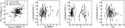
Left: the FJR that we derive (dashed) projected along the z-axis and the galaxies in the three samples of Treu et al. (2005), Auger et al. (2009) and Newman et al. (2010). We find no systematic biases in the FJR we derive. Centre left: the residuals of the velocity dispersions of the galaxies in the Auger et al. (2009) and Newman et al. (2010) samples as a function of effective radius. Centre right: the residuals of the velocity dispersions of the galaxies in the three samples as a function of redshift. The scatter in the residuals at z > 0.6 agrees with the scatter in the residuals at z < 0.6 within the uncertainties. Right: the residuals of the velocity dispersions as a function of the B-band magnitude.
The resultant FJR is consistent with B-band FJRs found from weak lensing analyses of Type Ia supernovae presented by Jönsson et al. (2010), Kleinheinrich et al. (2006) and Hoekstra, Yee & Gladders (2004). As a check of our FJR, we compare it with the i⋆-band FJR (which may be less prone to dust-extinction) presented by Bernardi et al. (2003) for all objects in GOODS. We find very close agreement between σ⋆ as inferred from the i-band FJR with our B-band FJR. For low-redshift objects, the scatter in the residuals between the two methods is 2 km s−1. For all objects out to z = 2, the scatter in the residuals between the two FJRs is 9 km s−1. This may be partially due to the Bernardi et al. (2003) FJR being calibrated at z ∼ 0, and not taking into account redshift evolution. There are no systematic biases in the residuals between these two FJRs as a function of z, MB or Re.
We compare our FJR with estimates of velocity dispersions using the stellar mass estimates of galaxies in our calibration sample using the relation between stellar mass and velocity dispersion presented by Hyde & Bernardi (2009b). We find the scatter in the residuals of velocity dispersion estimates using this method to be very similar (in fact, slightly larger) than those found using our FJR. This suggests that using stellar mass information rather than LB will not significantly reduce the scatter in our velocity dispersion estimates.
4 ASSESSING THE STRONG LENSING LIKELIHOOD OF LBGs
To quantify the strongly lensed fraction of LBGs, we model every foreground object in the field as a gravitational lens. Using photometric information of all foreground objects, we ask the following question for each LBG: What is the likelihood of this LBG being gravitationally lensed with magnification μ > 2 given its position relative to nearby (in projection) foreground objects? We disregard deflector–LBG pairs with a separation of θsep > 5.0 arcsec, which is much larger than the Einstein radius of typical deflectors. While the choice of maximum separation of 5.0 arcsec is somewhat arbitrary, we show in Section 5.2 that 5.0 arcsec is a reasonable choice. For each foreground object within 5.0 arcsec of the LBG, we use the following process.
Model the foreground object using a singular isothermal sphere (SIS) density profile.
Calculate the velocity dispersion that the foreground object requires for it to produce an image at the observed position of the LBG with a magnification of μ = 2, denoted by σ⋆, req. For an SIS, μ = 2 marks the beginning of the strong lensing regime. The required velocity dispersion depends on the LBG–deflector separation, LBG redshift and deflector redshift.
Calculate the likelihood that the foreground object has a velocity dispersion greater than or equal to σ⋆, req. This is the likelihood of strong lensing for that deflector–LBG pair.
Weight the likelihood of lensing by the inverse of the detection completeness at the separation between the LBG and the nearby foreground object.
The final step accounts for reduced sensitivity to faint LBGs nearby bright foregrounds. We explain this process further in Section 4.1.
We show a subset of the sample consisting of some of the highest-likelihood lenses in Fig. 2. We describe these systems further in Section 5.1.
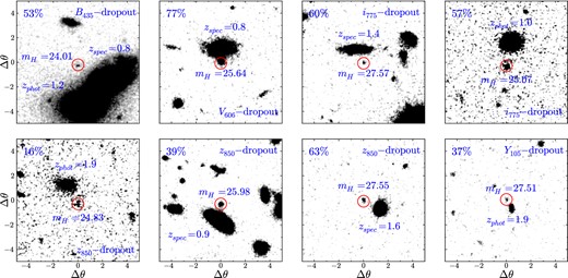
Examples of possibly lensed LBGs in the four samples. All cutouts are of the J125 images, are 10.0 × 10.0 arcsec and are shown on the same contrast scale (except for the top-left cutout, which contains two very bright foreground galaxies). The LBGs are circled in red and the deflectors are labelled by their spectroscopic/photometric redshifts. Each LBG is labelled with its H160 magnitude, and its likelihood of being strongly lensed (top-left corner). The LBG shown in the bottom-left panel is the brightest LBG in the z ∼ 7 sample.
4.1 Accounting for sensitivity variations
Faint LBG samples have a reduced completeness compared to bright ones. This alone would not affect our inference of the lensed fraction, because the completeness would change the numerator and the denominator by the same factor at fixed magnitude. However, we note that there may be a further reduced sensitivity to detecting faint LBGs around bright objects, which will affect potentially lensed LBGs differently to those isolated in the field. This effect could cause our measured strongly lensed fraction to be artificially low.
We weight all LBGs that appear close in projection to bright foreground objects by the inverse of their relative detection probability in order to account for reduced sensitivity around foreground objects. To do this, we run completeness simulations around all foreground objects which are either
assessed as having a greater than 1 per cent chance of lensing a nearby LBG, or
brighter than mr = 24 mag and within 2.5 arcsec of an LBG.
We run source recovery simulations in order to determine completeness as a function of radius around each foreground meeting either of the above criteria. The source recovery simulations are run for LBGs1 at the redshift and of the magnitude corresponding to that of the nearby LBG. The completeness of a source LBG, sc, becomes unaffected by typical foregrounds at a separation of around 1.5–2.0 arcsec. The weight, wc, we apply to each LBG is defined as the inverse of the completeness, wc ≡ 1/sc. We apply a maximum weighting of wc = 10 to any LBG.
We find that weighting the lensed fraction in this way has a minimal effect on the bright end of the observed lensed fraction. However, the relative completeness of faint galaxies near to bright foreground galaxies is, as expected, lower than for the brighter LBGs.
4.2 Uncertainty checks
The typical uncertainty in the photometric redshifts of foreground sources derived in the 3D-HST catalogues are Δz ∼ 0.1–0.2, so the uncertainty in the magnification is dominated by the intrinsic uncertainty in the FJR. Furthermore, the uncertainty in MB due to photometric redshift errors (via the distance modulus) is partially self-regulating as the inferred velocity dispersion is a decaying function of redshift, while inferred rest-frame luminosity is an increasing function. We find that of the 40 z ∼ 7 LBGs that have a likelihood of lensing of ≥10 per cent, the deflector of only one has a photometric redshift with less than an 80 per cent chance of residing within Δz = 0.2. None of the deflectors of z ∼ 4–6 LBGs with a likelihood of lensing of ≥10 per cent have photometric redshifts with less than an 80 per cent chance of residing within Δz = 0.2. The uncertainty in source redshift (Δz ∼ 0.35) is negligible as the angular diameter distance is a relatively flat function at high redshift.
There is a possible Eddington bias stemming from uncertainties in the photometry and the shape of the LF at z ∼ 1, which could bias the inference of σ⋆ from the B-band luminosity. We find that Ψ(L ± δL) only varies by 2–5 per cent from Ψ(L) for galaxies brighter than ∼M⋆ at z = 1 in the field. Therefore, the number density of bright galaxies does not change significantly within the photometric uncertainties, and the Eddington bias is negligible.
We note that a limitation of this analysis is that it assumes all deflectors to be SISs. Singular isothermal ellipsoids (SIEs) may be a more realistic parametrization of potential deflectors (see Keeton 2001, for ellipsoidal density parametrizations). However, SIEs do complicate the calculation significantly (Kormann, Schneider & Bartelmann 1994; Huterer, Keeton & Ma 2005). The median ellipticity for all objects in the CANDELS fields is |$\overline{\epsilon }=0.21$|, with 83 per cent having an ellipticity of ϵ < 0.4. In the case of low deflector ellipticity (ϵ ≲ 0.2), the change in the magnification estimate is ≈10 per cent along both the major (+10 per cent) and minor (−10 per cent) axes. For larger ellipticities (ϵ ≃ 0.4), the magnification estimate becomes ≈20 per cent lower for an image located along the minor axis, and a factor of 2 higher for images along the major axis. Using an elliptical deflector model for the system shown in the bottom, centre-left panel of Fig. 2, which includes a deflector with large ellipticity (ϵ = 0.48), we estimate the magnification to be μ ≃ 1.6, as compared with the SIS estimation of μ ≃ 1.8. The LBG in the bottom-right panel of Fig. 2, which is near a deflector with ellipticity ϵ = 0.33, has a magnification of μ ≃ 1.6 in the SIS model, which becomes μ ≃ 1.9 using an ellipsoidal model.
Similarly, the lensing cross-section (the strong lensing area in the image plane owing to a deflector) of an SIE is the same as the optical depth of an SIS with a higher order term (Kormann et al. 1994). The area of sky covered by the Einstein radius of an SIE is only ≈5 per cent larger than the area of sky covered by an SIS for reasonable ellipticities (ϵ ≲ 0.4). Therefore, our calculations of the optical depth in Section 6 are not significantly affected by the SIS assumption. These calculations are consistent with previous studies of the effect of ellipticity on the strong lensing optical depth and magnification, such as Huterer et al. (2005) who noted that aside from image multiplicities, introducing shear and ellipticity has surprisingly little effect. Hence, using an SIE deflector will not qualitatively change either our strongly lensed fraction or magnification bias results.
5 THE STRONGLY LENSED FRACTION
The method of prescribing a likelihood of strong lensing described in Section 4 was applied to each LBG in the samples at z ∼ 4, z ∼ 5, z ∼ 6 and z ∼ 7–8. The 455 z850 dropouts and 155 Y105 dropouts were combined to create a statistically significant sample with a mean redshift of |$\overline{z}=7.2$|. The number of strongly lensed LBGs brighter than a theoretical survey limit, mlim, is assessed for each of the samples. For the i775, and z850 & Y105 samples, we assess the lensed fraction brighter than mlim = 26, 27, 28, 29 and 30 mag in H160. We include mlim = 25 mag for the V606 sample and mlim = 24 and 25 for the B435 sample, as M⋆ appears brighter for these samples. The strongly lensed fraction is not affected by the differing depth of the CANDELS fields and the XDF.
The cumulative lensed fraction at each of these flux limits is the ratio of the expected number of strongly lensed LBGs (the sum of all lens likelihoods) brighter than the flux limit and the total number of LBGs appearing brighter than the flux limit. However, the cumulative lensed fraction depends on the total completeness of the combined sample. To account for incompleteness in number counts, we use the LF of Bouwens et al. (2014). The cumulative lensed fraction at z ∼ 4, z ∼ 5, z ∼ 6 and z ∼ 7 is shown in the left-hand panel of Fig. 3. The right-hand panel of Fig. 3 shows the observed magnification bias (see Section 6). When inferring properties of the LF (Sections 6.1 and 6.2) we use the observed lensed fraction in each bin without LF-correction so as to not presuppose the nature of the LF.
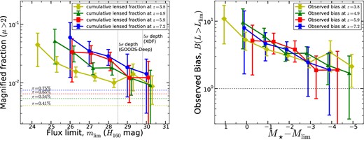
Left: the lensed fraction of background LBGs as a function of flux limit for the z850 and Y105-dropout samples (blue), i775-dropouts (red, offset by m + 0.1), V606-dropouts (green, offset by m + 0.2) and B435-dropouts (yellow, offset by m + 0.3). The observed lensed fraction decreases monotonically with decreasing redshift for flux limits of mlim = 26, 27, 28 and 30. The analytic strong lensing optical depths, τ, (strongly lensed fraction of random lines of sight) for each source redshift are plotted as dashed lines in the same colours as the observed lensed fractions (see Section 6). Right: the observed magnification bias at each redshift overlaid as a function of M⋆ − Mlim (see Section 6). The B435 sample contains the brightest measurements with respect to M⋆ (1 mag brighter), followed by the V606 sample, the z850 & Y105 sample and the i775 sample. The bias is defined as the ratio of the solid and dashed lines in the left-hand panel. We show the bias at each redshift individually in Fig. 5. For an LF without strong evolution in α, which is approximately observed from 4 < z < 7, the bias is not expected to evolve. A roughly constant bias is observed at all values of M⋆ − Mlim for the four independent LBG samples from 4 < z < 7.
The trend to a larger fraction of strongly lensed galaxies for brighter flux limits is reasonably smooth, monotonic and observed in each of the four independent samples. The amplitude at all flux limits steadily increases from z ∼ 4 to z ∼ 7 (although the error bars are large), which is expected as the faint-end slope steepens and the strong lensing optical depth increases at higher redshift. The excess probability of gravitational lensing of bright galaxies is detected at high significance in each of the samples. The lensed fraction of LBGs brighter than |$m_{H_{160}}=26$| is ∼6 per cent at z ∼ 7 and ∼3.5 per cent at z ∼ 6, although the uncertainty is large due to the rarity of bright objects at high redshift. At z ∼ 5, the lensed fraction at the same flux limit is ∼3.5 per cent and at z ∼ 4 the lensed fraction is ∼1.5 per cent.
We also assess the lensed fraction at brighter flux limits for the z ∼ 4 and z ∼ 5 samples. We find that the lensed fraction continues to rise, as expected. At z ∼ 5, ∼5 per cent of LBGs brighter than m = 25 are strongly lensed, and at z ∼ 4, ∼4.5 per cent of LBGs brighter than m = 24 are lensed.
The errors are calculated using bootstrap resampling. The bootstrap sample is drawn from the entire sample with replacement N = 104 times. Each time, each LBG is considered either ‘lensed’ or ‘not lensed’ randomly according to its likelihood of having been lensed. The lens fraction is recalculated for all limiting fluxes. The error bars represent the 1σ limits of the resultant distributions.
5.1 Examples of likely lensed systems
We present an illustrative sample of some likely lensed candidates in the surveys in Fig. 2. Cases from our highest-z sample are emphasized because they are of the most interest, and have the most importance to future surveys. We note that the three brightest z and Y-dropouts in the entire sample are each deemed to have a likelihood of lensing of >10 per cent. The brightest LBG in the z ∼ 7 sample is shown in the bottom-left panel of Fig. 2. All cutouts are shown at the same contrast scale, except for the z ∼ 4 lens candidate (top left), which is in proximity to two very bright foreground galaxies, both with MB ∼ −23.5, one of which is spectroscopically confirmed at z = 0.8. All cutouts are 10.0 arcsec on each side. In each case, the deflector candidate is labelled with its spectroscopic or photometric redshift and the LBG is labelled with its H160 magnitude.
The cutouts highlight the difficulty in locating secondary images in the event the LBG has been strongly lensed. A secondary image will appear closer to the foreground galaxy than the primary (circled) image, and is likely to also appear much fainter than the primary image.
5.2 Deflector properties
We present the distribution of the image–deflector separations, deflector redshifts and deflector B-band absolute magnitudes in this section. The number of lensed sources is weighted by the likelihood of lensing for each image–deflector configuration.
The top row of Fig. 4 shows the distribution of lens rest-frame B-band magnitudes for each of the four independent LBG samples. The peak of the distribution occurs around MB ∼ −22 for each of the samples.
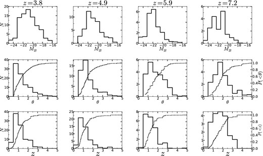
The lensing-likelihood-weighted distributions (solid) and cumulative distributions (dashed) of deflector properties. These distributions illustrate the diversity and evolution of the deflector population in the four samples analysed. Top row: the distribution of B-band absolute magnitudes of the deflectors for the four LBG samples. Middle row: the distribution of image–deflector separations for the four LBG samples. Bottom row: the distribution of redshifts of the deflectors for the four LBG samples.
The middle row of Fig. 4 shows the distribution of image–deflector separations for each of the LBG samples. The normalized cumulative fractions are shown as dashed lines. We observe an approximate increase in the peak of the separation distribution as redshift increases (from ∼1.0 arcsec at z ∼ 4 to ∼2.0 arcsec at z ∼ 7), consistent with the expectation that higher redshift sources have larger deflection angles.
The bottom row of Fig. 4 shows the distribution of deflector redshifts. The normalized cumulative fractions are shown as dashed lines. We observe an increase in the peak of the deflector redshift distribution from z ∼ 4 sources, where the deflector distribution peaks around z ∼ 1, to the z ∼ 7 sources, where the peak occurs around z ∼ 2. This evolution is consistent with the expectation that lenses are most likely to be found at around half of the angular diameter distance to the source.
6 MAGNIFICATION BIAS
The total magnification bias of a flux-limited sample, B(L > Llim), is the ratio of the fraction of strongly lensed galaxies and the fraction of strongly lensed random lines of sight, defined as the strong lensing optical depth, τ (e.g. Wyithe et al. 2011). We generate a catalogue of 50 000 random source positions in the GOODS fields and use the method of assessing the lensed fraction presented above in Section 4 to determine the fraction of the source plane that will be strongly lensed. Based on our FJR, we assess the strong lensing optical depth for sources at z ∼ 4, z ∼ 5, z ∼ 6 and z ∼ 7.2 to be τ = 0.41, 0.54, 0.65 and 0.75 per cent. The values found are broadly consistent with theoretical predictions of the strong lensing optical depths at these redshifts (Barkana & Loeb 2000; Wyithe et al. 2011; Mason et al. 2015). Due to the large number of foregrounds in the CANDELS fields, the relative statistical uncertainty on τ is only ∼4 per cent in all samples, and hence negligible in our bias calculations. We find consistent values for the optical depth if we apply a reasonable upper limit of ∼350 km s−1 on the inferred velocity dispersion of foreground galaxies. We find that our method of determining the optical depth returns values in close agreement with those in Mason et al. (2015) when we adopt their method of inferring velocity dispersions using stellar mass estimates.2 The optical depths are plotted as dashed lines in Fig. 3.
The bias is therefore the observed magnified fraction divided by the optical depth (the solid lines divided by the dashed lines in Fig. 3). The observed total bias for each of the samples at a range of flux limits is plotted in the right-hand panel of Fig. 3 and the top row of Fig. 5. The bias reaches values of ∼10 at bright magnitudes and high redshifts, but near the survey flux limit has values lower than expected for a LF that remains steep well beyond survey limits.
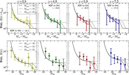
Top row: the observed total magnification bias of all galaxies brighter than a flux limit M⋆ − Mlim (solid) compared with the theoretical magnification bias for the LFs (described by equation 10) from Bouwens et al. (2014) with a range of magnitudes at which the LF flattens (α ∼ −1), denoted by Mturn. The cumulative lensed fraction is corrected for incompleteness according to the LF of Bouwens et al. (2014). Bottom row: the observed magnification bias in each bin plotted at the mean luminosity of the bin. At faint magnitudes in each sample of LBGs, the bias falls below the value expected from a faint-end slope continuing well beyond the survey limit, indicating a possible deviation from a steep faint-end slope of the LF, although they agree with theory within their error bars. For an LF with a steep faint-end slope continuing well beyond the flux limit, the bias flattens to a value of B ∼ 2–3 (depending on α). The measurements of bias at a fixed luminosity do not need to be corrected for incompleteness.
We calculate the observed magnification bias in each bin (as opposed to the total magnification bias for all galaxies brighter than a flux limit). The results are plotted in the bottom row of Fig. 5.
For an LF with weak (or no) redshift evolution of the α parameter, the magnification bias as a function of M⋆ − Mlim is expected to remain approximately constant with redshift. To highlight that this trend exists in the data, we plot the observed magnification bias at each redshift on the same axes in the right-hand panel of Fig. 3. While α evolves from ∼−1.6 to ∼−2.0 from z ∼ 4 to z ∼ 8, the statistical uncertainties in our measurements are larger than the change in bias from this evolution.
Results for our bias estimates given the Schechter LF parameters in Bouwens et al. (2014) and theoretical curves are plotted in Fig. 5. The top row compares the theoretical bias of all galaxies in a flux-limited sample with our measurements of the observed bias for all galaxies in a flux-limited sample. The bottom row shows the theoretical bias of galaxies at a fixed luminosity with our measurements of the observed bias in each magnitude bin. Theoretical values for bias are calculated using previously derived LF parameters α and M⋆ (Bouwens et al. 2014) and a range of values at which the LF deviates from a steep faint-end slope. We find close agreement between the observed shape and amplitude of the magnification bias and the theoretical function in each of the independent samples.
It is worth noting that the inferred magnification bias is not sensitive to the parameters of the FJR (Section 3), because the use of the FJR to determine the efficiency of observed galaxies affects both the numerator (fraction of strongly lensed LBGs) and the denominator (the strong lensing optical depth) similarly.
6.1 The faint-end slope beyond current flux limits
Magnification bias results from magnification of intrinsically faint sources below an observed flux limit into an observed sample, hence quantifying the degree of magnification bias offers an opportunity to investigate the behaviour of the LF beyond current survey limits.
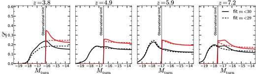
The inferred value of Mturn using the magnification bias measurements of all galaxies brighter than m < 30 (solid) and all galaxies brighter than m < 29 (dashed). The bias measurements which we fit to are shown in the bottom row of Fig. 5. In black we plot the likelihoods with a prior on α and M⋆ from Bouwens et al. (2014, see table 4 therein for values). The red curves show the estimated likelihoods including an additional requirement that the minimum magnitude is fainter than the magnitude to which current observations confirm a steep faint-end slope. We find approximately consistent preferred values of Mturn in each of the four samples, but with varying amplitudes. For LBGs brighter than m = 30 (approximately the 5σ XDF limit, solid line), we find a preferred value of Mturn around the observational limits in each sample. However, a value of Mturn > −16 is not excluded. For only LBGs brighter than m = 29 (dashed line), we find no constraint on Mturn in any of the samples. This is expected, because to constrain Mturn we need to consider galaxies within ∼1–2 mag of Mturn. The curves are normalized such that the probability of Mturn < −12 is unity.
We find that the constraint disappears when Mturn is fitted to only brighter (m < 29) galaxies. We extend this test by recalculating our results by omitting XDF LBGs entirely from the analysis to investigate whether the observed magnification bias will always approach unity near the flux limit due to selection effects. When we perform this test, we find the magnification bias of galaxies in the GOODS-North and GOODS-South is completely consistent with that of the full sample, rather than approaching unity near the flux limit.
It is important to note that the magnification bias is only observed to drop below its expected value close to the current flux limits where selection effects become significant. While we have taken care to account for the decreased sensitivity to very faint sources, there still exists the possibility that we have missed a significant fraction of gravitationally lensed LBGs at very faint magnitudes. Furthermore, if the interloper fraction at very faint fluxes is high, the lensed fraction will be underestimated, causing a spurious inference of Mturn.
The possibility of a flattening of the LF at Mturn ∼ −16.5 at z ∼ 7 is consistent with observations of LBGs down to MUV ∼ −15.5 of magnified z ∼ 7 LBGs using Frontier Fields cluster Abell 2744 (Atek et al. 2015; Ishigaki et al. 2015). Fig. 7 shows the Bouwens et al. (2014) and Atek et al. (2015) data with the best-fitting broken Schecter function (α2 = −1). We find that a broken Schechter function represents the data very well, and offers an independent constraint on Mturn. The data favour a value of Mturn ∼ −16.5, consistent with Mturn inferred from our magnification bias results. However, as is the case with our magnification bias analysis, this inference is based on a single data point.
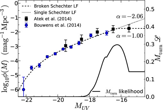
The z ∼ 7 LF data from Bouwens et al. (2014, blue circles) and Atek et al. (2015, black squares) with the best-fitting broken Schechter LF (dashed) and single Schechter LF (dotted). The solid line shows the likelihood of Mturn given the two data sets. We find a favoured flattening magnitude at MUV ∼ −16.5, consistent with our magnification bias measurements.
Further to this study at z ∼ 7, there exist measurements of the UV LF of z ∼ 2 LBGs down to MUV ∼ −13 (Alavi et al. 2014). While a single Schechter function favours a steep slope extending to MUV ∼ −13 at z ∼ 2, the shape of the LF at the faint end may be more complicated than this simple parametrization. In fact, the data also seem to suggest a flattening of the population density between −17 ≲ MUV ≲ −15, before a steeper upturn from −15 ≲ MUV ≲ −13 (see Alavi et al. 2014, fig. 7). This more complicated LF would produce a reduced magnification bias (B(L > Llim) ∼ 1) of z ∼ 2 LBGs near a flux limit of MUV ∼ −17.5, which is on the edge of current survey limits in blank fields (Reddy & Steidel 2009; Hathi et al. 2010; Oesch et al. 2010; Sawicki 2012). Additionally, a flattening, and potentially a rise in the LF at MUV ≳ −15 would not be inconsistent with the inference from GRB host galaxies studies (Tanvir et al. 2012; Trenti et al. 2012; Trenti, Perna & Tacchella 2013). In fact, these studies only constrain the presence of an abundant population of galaxies below the XDF detection limit, but not the shape of the galaxy LF, which they assume to be Schechter-like. Interestingly, theoretical models that are based on a double population of faint galaxies have been proposed in the context of hydrogen reionization (e.g. see Alvarez, Finlator & Trenti 2012).
6.2 Deriving Schechter parameters from lensing
A very interesting application of this analysis is that Schechter function parameters α and M⋆ can be derived directly from the magnification bias. This method is completely independent of the standard procedure using number counts of galaxies, and therefore could be combined to produce improved constraints.
The magnification bias at a fixed luminosity can be predicted using equation (8), and is a function of α and M⋆. By fitting the predicted bias of LBGs at a fixed flux to our measured bias in each flux bin (which is shown in the bottom row of Fig. 5, and is not the LF-corrected cumulative fraction), we can constrain α and M⋆.3 This does not rely on any prior knowledge of the LF. Because α and M⋆ are much more sensitive to the bias of bright galaxies than that of faint galaxies, and we see a possible deviation from a single Schechter function at faint magnitudes, we exclude the two faintest bins (29 < m < 30, and 28 < m < 29) from the fit.4 Fig. 8 shows the constraints on the LF from the observed magnification bias alone along with the constraints from number counts of the same samples.

Measurement of the Schechter parameters, α and M⋆, using only the observed magnification bias as a function of M⋆ − Mlim (black). The contours from Bouwens et al. (2014, red) and Finkelstein et al. (2014, yellow) are shown for comparison. We find close agreement between the two methods at z ∼ 4 and z ∼ 5, while the constraints at z ∼ 6 and z ∼ 7 from lensing are weaker due to the larger error bars on the magnification bias measurements.
The measurements of the bias at z ∼ 4 and z ∼ 5 do an excellent job of constraining the LF. At higher redshift, as the samples become smaller and the random errors grow, we cannot constrain the LF as effectively. However, we find that our observations are consistent with the UV LFs presented by Bouwens et al. (2014). This also provides an internal consistency check of our analysis.
6.3 Contaminant discussion
We check for bias arising from the selection of LBGs. There may be an enhancement and reddening of LBG candidates observed around bright, red foreground galaxies due to photometric scatter, causing an increased fraction of interlopers around such foreground objects and providing a false lensing signal among bright candidates. To determine if this may affect our results, we check if an enhanced interloper fraction around bright foregrounds is found in lower redshift LBG samples for which there exists spectroscopic follow-up. We combine catalogues with spectroscopically confirmed LBGs and photometrically selected LBGs which were identified as interlopers from 3 < z < 6 using observations reported by Vanzella et al. (2009), Reddy et al. (2006), Malhotra et al. (2005) and Steidel et al. (2003). We compare the fraction of interlopers for LBGs within 5.0 arcsec of bright, red foreground galaxies (mr < −22 mag) with the fraction of interlopers in the total sample. In both cases, we find the interloper fraction to be ∼8 per cent, with 2 of 25 LBGs around bright foreground galaxies identified as interlopers, and 21 of 252 of the entire sample. This indicates that the alignment between bright LBGs and massive foreground galaxies is not likely due to selection bias. The large enhancement in false identifications required to mimic the observed magnification bias of ∼10 for bright galaxies is clearly inconsistent with the spectroscopic data.
7 MAGNIFICATION BIAS AND THE LF
The effect of magnification bias on determining the LF is an important consideration when making a census of galaxies in the epoch of reionization (Wyithe et al. 2011; Mason et al. 2015). In this section, we show the effect that the lensed fraction reported in this paper has on the observed LF.
We begin by assuming that the observed LF is not affected by gravitational lensing and hence represent the intrinsic LFs. We plot these intrinsic LFs (Bouwens et al. 2014), the inferred observed LF and observations (Bouwens et al. 2014; Bowler et al. 2014) at z ∼ 4, z ∼ 5, z ∼ 6, z ∼ 7, z ∼ 8 and z ∼ 10 in Fig. 9 (dashed lines). Fig. 9 also shows the biased LFs, illustrating the luminosity at which gravitational lensing becomes important. This also illustrates the assumption that current LF measurements are not significantly affected by magnification bias is sound.
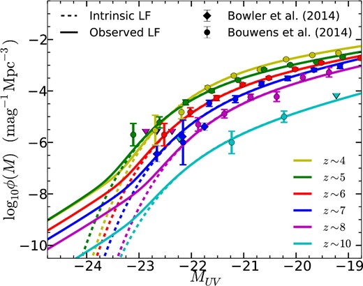
The effect of magnification bias on the bright end of the LFs z ∼ 4, z ∼ 5, z ∼ 6, z ∼ 7, z ∼ 8 and z ∼ 10 (LBGs become monotonically more abundant with decreasing redshift at MUV ≤ −22). The observed LFs are shown as solid lines, and the intrinsic LFs as dashed lines. The LF measurements from Bouwens et al. (2014) and Bowler et al. (2014) are plotted as circles and diamonds, respectively. At z ∼ 7, z ∼ 8 and z ∼ 10, observations are close to probing the bright end where gravitational lensing becomes a significant effect, but not bright enough for it to be manifested in the observed LF.
The effect of magnification bias is not significant at the faint end of the LF. At around 2 mag fainter than M⋆, the excess observed abundance of LBGs is of the order of 0.5 per cent for all of the samples, which is significantly smaller than the observational errors in the abundances at these magnitudes.
We note that even the brightest Bowler et al. (2014) and Bouwens et al. (2014) measurements are not bright enough to probe the affected region of the LF. However, the effect magnification bias will have on surveys at z ≳ 8 is obvious from the solid lines for z ∼ 8 and z ∼ 10 where the observed LF will display a break from the intrinsic LF around MUV ≲ −22.5.
Not plotted in Fig. 9 are extrapolated LFs at z > 10. Wyithe et al. (2011) showed that if M⋆ drops sharply at high redshifts, surveys of the depth of the XDF with JWST will observe galaxies at z > 10 in the affected region of the LF.
8 ANALYSIS OF CURRENT J125-DROPOUTS
In Section 7, we presented the effect that magnification bias has on the observed LF. Fig. 9 highlights that while magnification bias is not a significant effect in current surveys out to z ∼ 8, the affected region of the z ∼ 10 LF begins at around MUV ∼ −22.5. We investigated the four unusually bright z ∼ 10 J125-dropouts presented by Oesch et al. (2014) to search for evidence of lensing. This point is discussed in Oesch et al. (2014), where they find there is the possibility of a modest amount of lensing in two of the four dropouts. By applying the technique employed in this paper, we assign likelihoods of lensing to the four z ∼ 9–10 LBGs.
As noted by Oesch et al. (2014), two of the LBGs are not close in projection to any foreground objects (GN-z10-3 and GN-z9-1 in the notation of Oesch et al. 2014), while the other two do have projected neighbours (GN-z10-1 and GN-z10-2). GN-z10-1 is 1.2 arcsec from a foreground galaxy at zphot = 1.6 with MB = −20.1 (using photometry from the 3D-HST catalogue). Oesch et al. (2014) infer a photometric redshift of z = 1.8). Using our redshift-evolving FJR, this corresponds to a stellar velocity dispersion of 140 km s−1. The required stellar velocity dispersion for strong-lensing in this case is 198 km s−1, giving this LBG a likelihood of lensing of |$\scr {L}=0.12$|. GN-z10-2 is 2.9 arcsec from a bright galaxy at zspec = 1.02 with MB = −20.7. This corresponds to an inferred stellar velocity dispersion of 214 km s−1. The required stellar velocity dispersion for strong lensing is 279 km s−1, giving a likelihood of lensing of |$\scr {L}=0.1$|. While the statistics are too small to draw any firm conclusions, this average observed lensed fraction of ∼6 per cent for the four galaxies is consistent with a lensed fraction of LBGs brighter than M⋆ of ∼10 per cent.
9 SUMMARY
We have estimated the likelihood of strong gravitational lensing of LBGs in the XDF and GOODS at z ∼ 4, z ∼ 5, z ∼ 6 and z ∼ 7. We used a calibrated FJR to estimate the lensing potential of all foreground objects in the fields. The result is a measurement of significant magnification bias in current high-redshift samples of LBGs. Our analysis allows us to draw the following conclusions.
Approximately 6 per cent of LBGs at z ∼ 7 brighter than M⋆ (|$m_{H_{160}}\sim 26$| mag) are expected to have been strongly gravitationally lensed with μ > 2.
The observed strongly lensed fraction of LBGs at all values of |$m_{H_{160}}$| falls monotonically from z ∼ 7 to z ∼ 4, which can be explained by the expected evolution in the optical depth with redshift, and also M⋆ appearing brighter at lower redshift.
By evaluating the optical depth in our lensing framework, we calculate the magnification bias in each sample as a function of M⋆ − Mlim, and find that the results agree at each redshift and are well described by theoretical predictions.
Extrapolation of our analysis leads to expectations for an increased fraction of strongly lensed galaxies at z ≳ 8, consistent with Wyithe et al. (2011).
The magnification bias of the faintest LBGs in the sample suggests there may be a flattening of the faint-end slope below current detections limits (MUV ≳ −16.5). However, this result relies on LBG detections at low S/N in the XDF, and the constraints are weak. We present this result tentatively, with deeper data needed to better understand the population of faint high-z galaxies.
Assessing the magnification bias as a function of luminosity offers an independent method of determining Schechter parameters α and M⋆. The results from this method are consistent with those found by fitting the LF based on number counts.
With the confirmation of the role of magnification bias come important consequences for future surveys of galaxies at 10 < z < 20. Currently, the LFs at z ∼ 8 need not be corrected for magnification bias. However, magnification bias will be significant for LFs at z ≳ 10, notably in the JWST era (Wyithe et al. 2011). In particular, with M⋆ possibly dropping rapidly beyond z ∼ 8 (Oesch et al. 2014), JWST will identify predominantly gravitationally lensed galaxies at z ≳ 10.
JSBW is supported by an Australian Research Council Australian Laureate Fellowship. MT acknowledges support from the Australian Research Council through the award of a Future Fellowship. TT acknowledges support from the Packard Foundation via a Packard Fellowship. We thank Charlotte Mason for her useful comments and conversations. We also thank Adriano Fontana for his useful comments and suggestions.
The artificial sources in the recovery simulations are extended, and have sizes typical of LBGs at the appropriate redshift. It should be noted that strong lensing may cause the sources to appear more extended, which will affect their completeness. This effect is expected to be small, but is a slight limitation of this analysis.
We use stellar mass estimates of foreground galaxies in the GOODS/CANDELS fields from the 3D-HST catalogue.
We fit the theoretical bias at the mean magnitude of the LBGs in each magnitude bin to the observed bias in that bin with α and M⋆ as free parameters.
In fact, fitting the data including the two faintest bins with an extra free parameter, Mturn, and marginalizing over this parameter gives the same result.
REFERENCES
APPENDIX A: SPATIAL CORRELATIONS BETWEEN BRIGHT FOREGROUNDS AND LBGs
In this appendix, we present the manifestation of magnification bias in spatial correlations between bright foreground objects and bright LBGs, which illustrates the effect without relying on the FJR.
Source galaxies that have been magnified through gravitational lensing are necessarily located in close proximity to massive foreground objects. For the lensed fractions presented in Section 5, we expect there to be an excess density of bright LBGs around bright foreground objects over the average field density. As the lensed fraction decreases with decreasing luminosity, the excess probability around bright deflectors should also decrease. Similarly, the clustering around the more massive, brighter deflectors should be stronger than around less massive, fainter deflectors.
We compute the excess probability of finding an LBG brighter than m = 30, 28.5, 27.5 and 26.5 at |$\overline{z}=7.2$| within 5.0 arcsec of deflectors brighter than some MB. We choose 5.0 arcsec as our limit as this is approximately the image–deflector separation beyond which strong lensing is unlikely. This is confirmed by the distribution of separations shown in Fig. 4. We also present the spatial correlations for the lower redshift samples. At |$\overline{z}=5.9$|, we examine the same flux limits, at |$\overline{z}=4.9$| we replace mlim = 30 with mlim = 25.5 and at |$\overline{z}=3.8$| we replace mlim = 28.5 with mlim = 24.5. The results are plotted in Fig. A1.
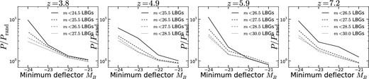
The excess probability of finding an LBG brighter than various flux limits within 5.0 arcsec of deflectors brighter than MB at z < 2. In each of the four samples, we find that there is an excess of LBGs around bright foreground objects. The excess becomes monotonically more pronounced with brighter flux limits around bright foregrounds in each of the four samples. At each redshift slice, we consider a different set of flux limits as M⋆ appears brighter for the lower redshift samples. The right-hand panel shows a large excess of bright LBGs at z ∼ 7 around bright foreground objects. At z ∼ 4, we find similar behaviour of bright LBGs appearing more frequently around bright foreground objects than in the total field, but the amplitude of the excess is much lower for the same flux limits of LBGs. However, for brighter flux limits, we see identical behaviour to that observed at higher redshift.
We find a large enhancement in the probability of finding bright LBGs nearby bright deflectors. As we consider fainter LBGs, the excess probability decreases monotonically in all of the samples. There exists a considerable excess of LBGs around foregrounds with MB < −23 at z ≥ 4, even for flux limits well beyond M⋆; however, this signal is driven mainly by the brightest LBGs. The excess likelihood of locating an LBG around a foreground approaches unity by MB ∼ −21 for all flux limits in all samples.
The clustering of bright LBGs nearby massive foreground galaxies is difficult to explain in the absence of magnification bias. One mechanism that could produce such a signal is the enhancement of LBGs around bright, red foregrounds. As discussed in Section 6.3, we searched for this effect in LBG samples with spectroscopic follow-up from the literature, and found no evidence that bright, red foregrounds enhance LBG detection. Therefore, we conclude that the proximity effect shown in Fig. A1 is consistent with being due to gravitational magnification of background LBGs by massive, bright foreground objects.
