


Abstract
Understanding the universal accretion history of dark matter haloes is the first step towards determining the origin of their structure. We use the extended Press–Schechter formalism to derive the halo mass accretion history from the growth rate of initial density perturbations. We show that the halo mass history is well described by an exponential function of redshift in the high-redshift regime. However, in the low-redshift regime the mass history follows a power law because the growth of density perturbations is halted in the dark energy dominated era due to the accelerated expansion of the Universe. We provide an analytic model that follows the expression |${M(z)=M_{0}(1+z)^{af(M_{0})}{\rm e}^{-f(M_{0})z}}$|, where M0 = M(z = 0), a depends on cosmology and f(M0) depends only on the linear matter power spectrum. The analytic model does not rely on calibration against numerical simulations and is suitable for any cosmology. We compare our model with the latest empirical models for the mass accretion history in the literature and find very good agreement. We provide numerical routines for the model online (available at https://bitbucket.org/astroduff/commah).
1 INTRODUCTION
Throughout the last decade, there have been many attempts to quantify halo mass accretion histories using catalogues of haloes from numerical simulations (Wechsler et al. 2002; McBride, Fakhouri & Ma 2009; Wang & White 2009; Fakhouri, Ma & Boylan-Kolchin 2010; Genel et al. 2010; Faucher-Giguère, Kereš & Ma 2011; van de Voort et al. 2011; Benson et al. 2012; Johansson 2013; Behroozi, Wechsler & Conroy 2013; Wu et al. 2013). Wechsler et al. (2002) characterized the mass history of haloes more massive than 1012 M⊙ at z = 0 using a one-parameter exponential form eβz. In their work, Wechsler et al. (2002) limited their analysis to the build-up of clusters through progenitors already larger than the Milky Way halo. Similarly, McBride et al. (2009) limited their analysis to massive haloes and found that a large fraction were better fitted when an additional factor of (1 + z)α was added to the Wechsler et al. (2002) exponential parametrization, yielding a mass history of the form M ∝ (1 + z)αeβz. Wong & Taylor (2012) investigated whether the mass history can be described by a single parameter function or whether more variables are required. They utilized principal component analysis and found that despite the fact that the McBride et al. (2009) two-parameter formula presents an excellent fit to halo mass histories, the parameters α and β are not a natural choice of variables as they are strongly correlated. Recently, van den Bosch et al. (2014) studied halo mass histories extracted from N-body simulations and semi-analytical merger trees. However, so far no universal and physically motivated model of a universal halo mass history function has been provided.
An alternative method to interpret the complex numerical results and to unravel the physics behind halo mass growth, is the extended Press–Schechter (EPS) formalism. EPS theory provides a framework that allows us to connect the halo mass accretion history to the initial density perturbations. Neistein, van den Bosch & Dekel (2006) showed in their work that it is possible to create halo mass histories directly from EPS formalism by deriving a useful analytic approximation for the average halo mass growth. In this work, we aim to provide a physical explanation for the ‘shape’ of the halo mass history using the EPS theory and the analytic formulation of Neistein et al. (2006). The resulting model for the halo mass history, which is suitable for any cosmology, depends mainly on the linear power spectrum.
This paper is organized as follows. We show in Section 2 that the halo mass history is naturally described by a power law and an exponential as originally suggested from fits to cosmological simulation data by McBride et al. (2009). We then provide a simple analytic model based on the EPS formalism and compare it to the latest empirical halo mass history models from the literature. Finally, we provide a summary of formulae and discuss our main findings in Section 3.
In a companion paper, Correa et al. (2015a, hereafter Paper II), we explore the relation between the structure of the inner dark matter halo and halo mass history using a suite of cosmological simulations. We provide a semi-analytic model for halo mass history that combines analytic relations for the concentration and formation time with fits to simulations, to relate halo structure to the mass accretion history. This semi-analytic model has the functional form, M = M0(1 + z)αeβz, where the parameters α and β are directly correlated with the dark matter halo concentration. Finally, in a forthcoming paper (Correa et al. 2015b, hereafter Paper III), we combine the semi-analytic model of halo mass history with the analytic model described in Section 2.3 of this paper to predict the concentration–mass relation and its dependence on cosmology.
2 ANALYTIC MODEL FOR THE HALO MASS HISTORY
In order to provide a physical motivation for the ‘shape’ of the halo mass history, we begin in Section 2.1 with an analytic study of dark matter halo growth using the EPS formalism (Bond et al. 1991; Lacey & Cole 1993). In Section 2.2, we show that the halo mass history is well described by an exponential at high redshift, and by a power law at low redshift. In Section 2.3, we then adopt the power-law exponential form and use it to provide a simple analytic model for halo mass histories. Finally, we compare our results with the latest models of halo mass history from the literature in Section 2.4.
2.1 Theoretical background of EPS theory
The EPS formalism is an extension of the Press–Schechter (PS) formalism (Press & Schechter 1974), which provides an approximate description of the statistics of merger trees using a stochastic process. The EPS formalism has been widely used in algorithms for the construction of random realizations of merger trees (Kauffmann & White 1993; Benson, Kamionkowski & Hassani 2005; Cole et al. 2008; Neistein & Dekel 2008).
2.2 Mass accretion in the high- and low-z regimes
In this section, we analyse how the evolution of MEPS(z) given by equation (6) is governed by the growth factor. We provide two practical approximations for the growth factor in the high- and low-redshift regimes and investigate the ‘shape’ of MEPS(z) in these regimes by integrating equation (6).
In addition to the redshift dependence of the growth factor (D(z)), in equation (6) an extra redshift dependence is introduced through the quantity [Sq − S]−1/2 = [S(M(z)/q) − S(M(z))]−1/2. Before integrating equation (6), we calculate how the value of [S(M(z)/q) − S(M(z))]−1/2 changes with redshift to find a suitable first-order approximation to simplify the calculations.
Given the weak dependence on mass in the right part of equation (9), we simplify the expression [S(M(z)/q) − S(M(z))]−1/2 in our analysis using the approximation [S(M(z)/q) − S(M(z))]−1/2 ≈ [S(M0/q) − S(M0)]−1/2. It is important to note that as the MEPS(z) evolution (given by equation 6) is only governed by the growth factor in equation (2), we find that in the latter part of the accretion history, where most mass is accreted, the approximation [S(M(z)/q) − S(M(z))]−1/2 ≈ [S(M0/q) − S(M0)]−1/2, will carry an ∼5 per cent error for M(z) ≤ 1012 M⊙ and 15 per cent error for M(z) > 1012 M⊙. Earlier in the accretion history, the errors may be as large as ∼20 per cent and 40 per cent for M(z) ≤ 1012 M⊙ and M(z) > 1012 M⊙, respectively. We demonstrate in Section 2.4 that these errors do not affect the final M(z) model, which we show provides very good agreement with simulation-based mass history models from the literature.
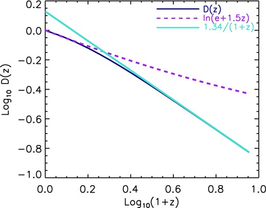
Linear growth factor against redshift. The dark blue solid line shows the growth factor obtained by performing the integral given by equation (2). The purple dashed line corresponds to the low-redshift approximation in equation (8). Similarly, the green solid line shows the approximation of the growth factor in the high-redshift regime.
Therefore, in the low-redshift regime, a power law (M(z) ∼ (1 + z)α) is necessary because the growth of density perturbations is halted in the dark energy dominated era due to the accelerated expansion of the Universe.
2.3 Analytic mass accretion history model based on the EPS formalism
The top panel of Fig. 2 shows a comparison between the analytic model given by equations (19)–(23) (blue solid line), and the limiting case for the halo mass histories given by equation (11) for the low-redshift regime (purple dashed line) and by equation (10) for the high-redshift regime (green solid line). In the last case, we renormalized the mass history curve to match that given by the analytic model at z = 7. This figure demonstrates how exponential growth dominates the mass history at high redshift, and power-law growth dominates at low redshift, as concluded in the previous section.
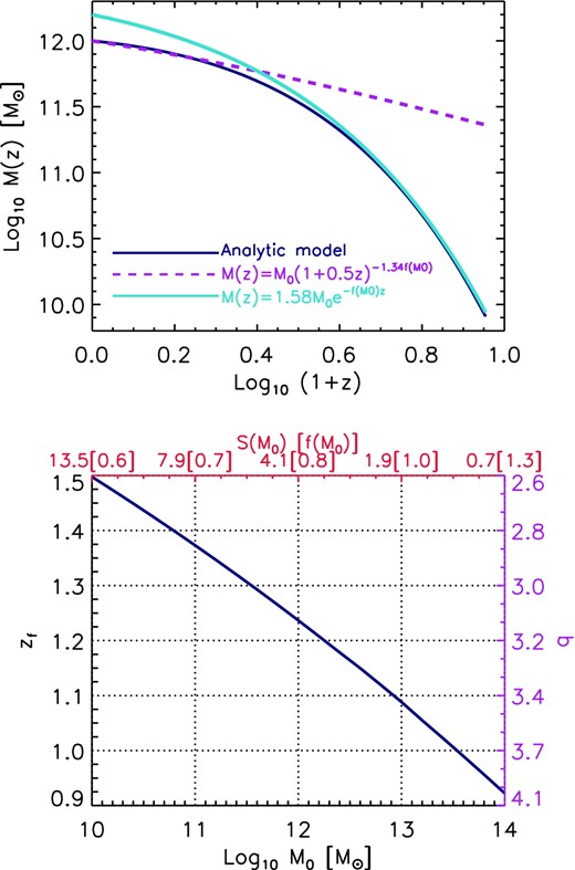
Top panel: comparison between halo mass histories predicted by the analytic model |$M(z)=M_{0}(1+z)^{af(M_{0})}{\rm e}^{-f(M_{0})z}$|, given by equations (19)–(23) (blue solid line), and the approximated halo mass histories given by equation (11), for the low-redshift regime (purple dashed line), and by equation (10), for the high-redshift regime (green solid line). Bottom panel: formation redshift against halo mass. Here the formation redshifts were obtained by solving equations (16) and (18). The right Y-axis shows the values of ‘q’ obtained when calculating the formation redshift, whereas the top X-axis shows the variance of the smoothed density field of a region that encloses the mass indicated by the bottom X-axis. The values of the function |$f(M_{0})=1/\sqrt{S(M_{0}/q)-S(M_{0})}$| are shown in brackets.
The bottom panel of Fig. 2 shows the formation time obtained from equations (16) and (18), as a function of halo mass. As expected, larger mass haloes form later. The right Y-axis shows the values of q obtained when calculating formation time, whereas the top X-axis shows the variance of the smoothed density field of a region that encloses the mass indicated by the bottom X-axis. The values of the function |$f(M_{0})=1/\sqrt{S(M_{0}/q)-S(M_{0})}$| are included in brackets. As can be seen from this figure, the larger the halo mass, the lower the variance S(M0), the larger f(M0), and so the larger the factor in the exponential that makes the halo mass halt its rapid growth at low redshift. For example, a 1014 M⊙ halo has a mass history mostly characterized by an exponential growth (|${\sim } {\rm e}^{-f(M_{0})z}$|) until redshift z = 1/f(M0) = 0.7, whereas a 1010 M⊙ halo only has an exponential growth until redshift z = 1.6. Note, however, that our analytic model is not limited to the halo mass ranges shown in the bottom panel of Fig. 2, it can be extended to any halo masses and redshifts and the q–M0 and |$\tilde{z}_{\rm f}{\rm -}M_{0}$| relations still hold.
The physical relation derived between the parameters describing the exponential and power-law behaviour implies that a single parameter accretion history formula should be seen in numerical simulations. In Paper II, we investigate the α and β parameter dependence in more detail, and we determine the intrinsic relation (which cannot be explored under the EPS formalism) between halo assembly history and inner halo structure.
2.4 Comparison with previous studies
In this section, we briefly describe the simulation-based halo mass history models presented in van den Bosch et al. (2014, hereafter vdB14) and McBride et al. (2009, hereafter MB09), and contrast them with our analytic model given by equations (19)–(23). Fig. 3 shows a comparison of our mass history model (turquoise solid lines) to the models of vdB14 (purple dashed lines) and MB09 (dark blue solid lines). vdB14 used the mass histories from the Bolshoi simulation (Klypin, Trujillo-Gomez & Primack 2011) and extrapolated them below the resolution limit using EPS merger trees. They then used a semi-analytic model to transform the average or median mass accretion history for a halo of a particular mass taken from the Bolshoi simulation, to another cosmology, via a simple transformation of the time coordinate. Using their publicly available code, we calculated the mass histories of 109, 1011, 1013 and 1015 M⊙ haloes for the WMAP1 cosmology. We find good agreement between our model and vbB14 for all halo masses. The main difference occurs for the mass histories of high-mass haloes (M0 > 1013 M⊙), where vdB14 seems to underpredict the mass growth above z = 4 by a factor of ∼1.2. In addition, vdB14 compared their model to those of Zhao et al. (2009) and Giocoli, Tormen & Sheth (2012), and found that both works predict smaller halo mass growth at z > 1.5.
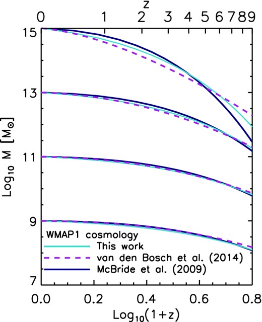
Comparison of halo mass history models. The analytic model presented in this work (turquoise solid lines) is compared with the median mass history obtained from the Bolshoi simulation and merger trees from vdB14 (purple dashed lines) and the best-fitting relations from the Millennium simulation from MB09 (dark blue solid lines). The comparisons are shown for four halo masses and for consistency with MB09 we assumed in our model and in the vdB14 model the WMAP1 cosmology.
We also compare our model to the MB09 mass history curves. MB09 used the Millennium simulation (Springel 2005) and separated their halo sample into categories depending on the ‘shape’ of the mass histories, from late-time growth that is steeper than exponential to shallow growth. We find that the fitting function that best matches our results is from their type IV category. We find good agreement with the MB09 formula.
Fig. 3 demonstrates that the physically motivated analytic model presented in this work yields mass histories that are in good agreement with the results obtained from numerical simulations. However, in contrast to the models based on fits to simulation results, our analytic model can be extrapolated to very low masses and is suitable for any cosmology.
3 SUMMARY AND CONCLUSION
We found very good agreement between the halo mass histories predicted by our analytic model and published fits to simulation results (Fig. 3). The reader may find a step-by-step description on how to implement both models in Appendix B, as well as numerical routines online.2
The relation of the parameters α and β with the linear power spectrum explains the correlation between the dark matter halo concentration and the linear rms fluctuation of the primordial density field that was previously noted in numerical simulations (Prada et al. 2012; Diemer & Kravtsov 2015). We show it in Paper II, where we derive a semi-analytic model for the halo mass history that relates halo structure to the mass accretion history. In that work, we combine the semi-analytic model with the analytic model presented here to establish the physical link between halo concentrations and the initial density perturbation field. Finally, in Paper III we combine the analytic and semi-analytic description to predict the concentration–mass relation of haloes and its dependence on cosmology.
We are grateful to the referee Aaron Ludlow for fruitful comments that substantially improved the original manuscript. CAC acknowledges the support of the 2013 John Hodgson Scholarship and the hospitality of Leiden Observatory. JSBW is supported by an Australian Research Council Laureate Fellowship. JS acknowledges support by the European Research Council under the European Union's Seventh Framework Programme (FP7/2007-2013)/ERC Grant agreement 278594-GasAroundGalaxies. We are grateful to the OWLS team for their help with the simulations.
Available at https://bitbucket.org/astroduff/commah.
REFERENCES
APPENDIX A: DIFFERENTIAL EQUATION FOR MEPS
APPENDIX B: Step-by-step guide to compute halo mass histories
B0.1 Analytic model based on EPS
This appendix provides a step-by-step procedure that details how to calculate the halo mass histories using the analytic model presented in Section 2.
Calculate the linear power spectrum P(k). In this work, we use the approximation of Eisenstein & Hu (1998).
- Perform the integral(B1)\begin{equation} S(R)=\frac{1}{2\pi ^{2}}\int _{0}^{\infty }P(k)\hat{W}^{2}(k;R)k^{2}{\rm d}k, \end{equation}
where |$\hat{W}^{2}(k;R)$| is the Fourier transform of a top hat window function and R defines S in a sphere of mass M = (4π/3)ρm, 0R3, where ρm, 0 is the mean background density today.
- Given M0, the halo mass today, calculate the mass history by first obtaining |$\tilde{z}_{\rm f}$|and(B2)\begin{equation} \tilde{z}_{\rm f}=-0.0064(\log _{10}M_{0})^{2}+0.0237(\log _{10}M_{0})+1.8837 \end{equation}(B3)\begin{equation} q=4.137\tilde{z}^{-0.9476}_{{\rm f}}. \end{equation}
- Use the parameter q to calculate f(M0), the function that relates the power spectrum to the mass history through the mass variance S,(B4)\begin{equation} f(M_{0})=1/\sqrt{S(M_{0}/q)-S(M_{0})}. \end{equation}
- Finally, the mass history can be calculated as follows,(B5)\begin{eqnarray} M(z)&=&M_{0}(1+z)^{af(M_{0})}{\rm e}^{-f(M_{0})z}, \end{eqnarray}where dD/dz is the derivative of the linear growth factor, which can be computed by performing the integral(B6)\begin{eqnarray} a&=&\left[1.686(2/\pi )^{1/2}\frac{{\rm d}D}{{\rm d}z}|_{z=0}+1\right], \end{eqnarray}D(z) is normalized to unity at the present.(B7)\begin{equation} D(z)\propto H(z)\int _{z}^{\infty }\frac{1+z^{\prime }}{H(z^{\prime })^{3}}{\rm d}z^{\prime }. \end{equation}
The above model is suitable for any adopted cosmology and halo mass range.
