


Abstract
We explore spectral properties of a two-component advective flow around a neutron star. We compute the effects of thermal Comptonization of soft photons emitted from a Keplerian disc and the boundary layer of the neutron star by the post-shock region of a sub-Keplerian flow, formed due to the centrifugal barrier. The shock location Xs is also the inner edge of the Keplerian disc. We compute a series of realistic spectra assuming a set of electron temperatures of the post-shock region TCE, the temperature of the Normal BOundary Layer (NBOL) TNS of the neutron star and the shock location Xs. These parameters depend on the disc and halo accretion rates (|$\dot{m}_{{\rm d}}$| and |$\dot{m}_{{\rm h}}$|, respectively) that control the resultant spectra. We find that the spectrum becomes harder when |$\dot{m}_{\rm h}$| is increased. The spectrum is controlled strongly by TNS due to its proximity to the Comptonizing cloud since photons emitted from the NBOL cool down the post-shock region very effectively. We also show the evidence of spectral hardening as the inclination angle of the disc is increased.
1 INTRODUCTION
The theoretical modelling and spectral studies of compact objects go hand in hand in understanding the accretion processes. In the past twenty five years, theoretical studies of accretion on to black holes have reached a very satisfactory stage (for a recent review, see Chakrabarti 2016) where it was shown that multiple aspects of observations of a large number of objects can be explained within a single framework. However, similar studies for a neutron star (NS) accretion have not been done, primarily because it is inherently more complex. First, an NS can have a magnetic field that interacts with the accretion flow. If it is strong enough, it can block direct accretion and the flow then approaches the star through the poles. Secondly, it has a hard surface that can have a range of temperatures thereby posing a difficult boundary value problem. The matter has to stop on the surface in the corotating frame with the star. In other words, independent of its past history, its final leg of journey must be sub-sonic and may form a boundary layer. In contrast, a black hole accretion flow always enters through the horizon with a velocity of light and is always supersonic. Another important difference is that while for a black hole accretion, there could be one single centrifugal barrier supported shock in a transonic flow, in an NS, there could be two shocks, one at a similar distance (in dimensionless unit) as in a black hole accretion and the other one right outside the hard surface (Chakrabarti 1989; Chakrabarti & Sahu 1997) of the star formed due to the boundary condition. The outer one is known as the CENtrifugal barrier supported BOundary Layer (CENBOL) and the inner one may be called the Normal BOundary Layer (NBOL). Thus, in a black hole accretion, energy is dissipated at the CENBOL and jets/outflows are produced there as well. In an NS accretion, both the boundary layers can take part in dissipating the compressional heat of thermal electrons. So the spectral properties are more complex. One interesting common theme, as far as the mathematical properties go, is that both the flows are sub-Keplerian at the very inner edge: For NS the sub-Keplerian nature is required to adjust with the sub-Keplerian rotation of the surface; while for black holes, the passage through the inner sonic point ensures that the flow is sub-Keplerian. Thus, a thorough fundamental understanding of the accretion flow is important. This paper is the first study to explore these aspects.
The most complete theoretical solution in the presence of advection, radiative transfer and heating is a transonic or advective flow (Chakrabarti 1990; Chakrabarti 1996, hereafter C96), which self-consistently passes through one or more sonic points. It was shown that in the absence of a significant viscosity, the flow will have a steady or oscillating shock but it would disappear when viscosity is high and the flow would be similar to a standard Shakura & Sunyaev (1973 , hereafter SS73) disc. Chakrabarti & Titarchuk (1995, hereafter CT95), used the two-component advective flow (TCAF) solution to show that spectral states of black holes could be understood by changes in the two independent accretion rates. Indeed, numerical simulations of Giri & Chakrabarti (2013) and Giri, Garain & Chakrabarti (2015) show that the two components are naturally produced when there is a vertical gradient of viscosity parameter. It was shown that when the viscosity parameter is higher than the critical value in the equatorial region, a standard Keplerian disc (KD) is formed flanked vertically by an advective sub-Keplerian halo as already envisaged before (C96).
Historically, the explanation of soft state spectra of NSs demanded the presence of a blackbody emission from the boundary layer of an NS (Mitsuda et al. 1984). For the harder states with a power-law tail in the energy spectrum, the need of Compton scattering became evident (White et al. 1986; Mitsuda et al. 1989). The difference between these two models was that while the former assumed a cooler boundary layer, the latter assumed a hotter one, compared to the accretion disc. Sunyaev and his collaborators (Inogamov & Sunyaev 1999, hereafter IS99; Popham & Sunyaev 2001, hereafter PS01; Gilfanov & Sunyaev 2014 , hereafter GS14) assume that the KD reaches all the way to the NS and is connected with the boundary layer where the thickness increases due to higher temperature. Most of these studies were done to address the soft state spectra of NSs. The state transition of NSs in Low Mass X-ray Binaries (LMXBs), presented another problem. The fact that disc accretion rate was not the single factor that controlled the size or temperature of the Compton cloud, used to model the hard state spectra, lead to the conclusion that some unknown parameter, related to the truncation radius of the disc, is responsible for the hard X-ray tail (Barret 2001; Barret & Olive 2002; Di Salvo & Stella 2002). Paizis et al. (2006) found a systematic positive correlation between the X-ray hard tail and the radio luminosity, inferring that the Compton cloud might serve as the base of radio jets (see Chakrabarti 2016, and references therein). Recent phenomenological works places a transition layer (TL) or Compton cloud between the KD and the boundary layer (Farinelli et al. 2008; Titarchuk, Seifina & Shrader 2014, hereafter TSS14). It has been argued in the past (Chakrabarti 1989; C96; Chakrabarti & Sahu 1997) that while in black hole accretion, passing of the flow through the inner sonic point ensures that the flow becomes sub-Keplerian just outside the horizon, in the case of NSs, the Keplerian flow velocity must slow down to match with the sub-Keplerian surface velocity. Numerical simulations clearly showed that jumping from a KD to a sub-Keplerian disc is mediated by a super-Keplerian region (Chakrabarti & Molteni 1995). In Titarchuk, Lapidus & Muslimov (1998, hereafter TLM98), a super-Keplerian TL was invoked to explain the kHz quasi-periodic oscillations (QPOs) and in TSS14 the TL was expanded several fold to explain the spectral properties. In reality, there are two such layers simultaneously present in an NS accretion: One is similar to the NBOL and the other is similar to the CENBOL in a black hole accretion (CT95). In a black hole accretion, only CENBOL is present. All these approaches clearly point to the existence of a CENBOL type hot electron reservoir, which naturally occurred in black hole accretion, confirming Chakrabarti & Sahu (1997) conclusions that the solutions of the transonic flows are modified only in the last few Schwarzschild radii as per the boundary condition of the gravitating object.
Monte Carlo simulations are essential in generating and understanding spectra emergent from highly non-local processes such as Comptonization. Toy models were made of spherical Compton clouds of constant temperature and optical depth, surrounding a weakly magnetic NS to generate hard X-ray tails (Seon et al. 1994). In case of NSs with strong magnetic fields (B ∼ 1010–1012 G), matter lands at the poles through the accretion column and the use of such a geometry leads to the successful explanation of spectral properties (Odaka et al. 2013, 2014) in certain cases. Although these studies provide some answers, so far, the spectral fitting carried out were based on phenomenological models that used an arbitrarily placed Compton cloud. TLM98 explained high-frequency QPOs considering a TL, and an extended TL was used to explain spectra using COMPTT and COMPTB models. Out of the two COMPTB components used, the one corresponding to Comptonization of NSs surface photons, showed a saturation in COMPTB models spectral index (Farinelli & Titarchuk 2011, hereafter FT11). The ‘Spectral slope/index’ in the context of COMPTB model, refers to α which is the slope of Comptonized component of the spectrum (=Γ − 1, the photon index). In this paper, we uniformly use the actual slope of the linear region of the spectrum (which includes both the primary and Comptonized photons) in log–log scale. Thus, the two terms do not represent the same quantity. Many NS LMXBs are studied using this framework, such as 4U 1728-34 (Seifina et al. 2011), GX 3+1 (Seifina & Titarchuk 2012, hereafter ST12), GX 339+0 (Seifina, Titarchuk & Frontera 2013, hereafter STF13), 4U 1820-30 (Titarchuk, Seifina & Frontera 2013, hereafter TSF13), Scorpius X-1 (TSS14), 4U 1705-44 (Seifina et al. 2015, hereafter STSS15), etc. Recently, the HMXB 4U 1700-37 has also been examined using the same model (Seifina, Titarchuk & Shaposhnikov 2016, hereafter STS16). This useful model to fit the spectra of NSs give the average temperature of the Compton cloud placed in between the disc and the NS surface, unlike what the TL used just outside the star. With an independent advective flow as in TCAF, the phenomenological Compton cloud is naturally explained without having to modify the earlier models drastically. Indeed, since the flow at the outer edge of the disc has little knowledge of the nature of the compact source, except near the innermost boundary, the overall flow configuration is not expected to be very different, especially when the magnetic field is weak (<108 G). The gravity simply lets the advective matter to fall almost freely till the surface of the star is hit.
In this paper, we study spectral properties of an NS in the presence of TCAF, which has a CENBOL as well as the NBOL of the star. A preliminary report has been presented in Bhattacharjee, Chakrabarti & Banerjee (2016). We use the size of the CENBOL (Xs), accretion rates of the KD and the sub-Keplerian halo as the free parameters. Additional parameters in the present context are the mass of the NS and the temperature of the NBOL. In the next section, we present a brief introduction to the TCAF solution around a black hole and how the solution is modified when the black hole is replaced by an NS. In Section 3, we describe the system in detail and define the properties of the NBOL, CENBOL and the KD. In Section 4, we describe, in brief, the Monte Carlo simulation procedure used in thermal Comptonization. The resultant spectra of the flow as a function of the flow parameters are given in Section 5. Finally, in Section 6, we give our concluding remarks.
2 TWO-COMPONENT FLOWS AROUND NSS
It is well known that the spectral and timing properties of a black hole cannot be explained by a standard KD alone (Sunyaev & Truemper 1979; Sunyaev & Titarchuk 1980, 1985; Chakrabarti & Wiita 1993; Haardt & Maraschi 1993; Chakrabarti & Titarchuk 1995; Chakrabarti 1997; Zdziarski 2003). A spectrum clearly has a thermal component resembling of a multicolour blackbody radiation. However, the other component is similar to a power-law component, which is produced by inverse Comptonization of the thermal or non-thermal electrons (Sunyaev & Titarchuk 1980, 1985). There are many models in the literature that present possible scenarios of how the electron cloud might be produced. However, there is a unique self-consistent solution, namely, the transonic flow solution based TCAF that addresses all the aspects of spectral and temporal properties at the same time. In this scenario, a CENBOL is produced very close to a compact object in the low-viscosity advection component. The boundary of CENBOL is a shock transition which may or may not be stationary. The post-shock region is a natural reservoir of hot electrons. Higher viscosity flow component near the equatorial plane becomes a KD and emits a multicolour blackbody radiation, which are intercepted and re-radiated by the CENBOL to create the power law like component which normally has an exponential cut-off where recoil becomes important. When the shock oscillates due to resonance (Molteni, Sponholz & Chakrabarti 1996) or non-satisfaction of Rankine–Hugoniot condition (Ryu, Chakrabarti & Molteni 1997), the resulting hard X-ray intensity is modulated with the size of the CENBOL and manifest as the low-frequency quasi-Periodic oscillations (LFQPOs). The CENBOL is also the source of outflows and jets, in that, when the CENBOL is cooled down due to excessive soft photons, the jet itself also disappears. There are clear observational evidence of two-component advective flows in several black hole candidates (Smith et al. 2001; Smith, Heindl & Swank 2002; Debnath, Chakrabarti & Mondal 2013a; Mondal, Debnath and Chakrabarti, 2014; Dutta & Chakrabarti 2016).
Since the nature of the companion remains generally similar irrespective of whether the compact object is a black hole or an NS, it is natural that we invoke the TCAF solution for the NSs as well, specifically when the magnetic field is not very strong. However, in addition to the CENBOL, to satisfy the inner boundary condition, the flow would have an optically thick boundary layer of the NS, which would also emit a characteristic blackbody radiation. These photons would be inverse Comptonized by the electrons inside the CENBOL, cooling it down further and making the spectra softer. In presence of a stronger magnetic field, a hot corona is produced when matter proceeds to the magnetic poles of the NS. This is also the region of inverse Comptonization. However, discussion on this case will require inclusion of synchrotron radiation, which is beyond the scope of this paper. In our solution, the Compton cloud is always a very hot reservoir of electrons (as compared to the NBOL or the KD), unless it is cooled down by the disc and/or NBOL.
3 MONTE CARLO SIMULATION OF TCAF AROUND A NEUTRON STAR
3.1 Simulation setup
In earlier papers from our group, Monte Carlo simulation results of TCAFs around black holes were presented (Ghosh, Chakrabarti & Laurent 2009; Ghosh et al. 2010, hereafter GCL09 and GGCL10, respectively). In the present context, in addition to the components used earlier, we must include a boundary layer (NBOL) of the star that will emit a blackbody radiation. In Fig. 1, we present the flow configuration of our simulation. We also use a more realistic post-shock region or CENBOL, namely, one that resembles a thick accretion disc (Molteni, Lanzafame & Chakrabarti 1994). Since we are considering a stationary configuration, to begin with, we use the density and temperature distribution as specified by Chakrabarti (1985) inside a general relativistic model of the thick accretion disc.
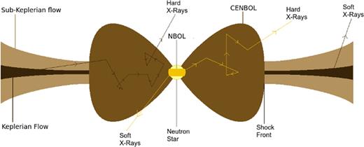
A schematic diagram of the two-component advective flow (TCAF) around an NS. The KD and the boundary layer on the surface of the NS (NBOL) emit soft blackbody photons, which are scattered by the hot electrons in the centrifugal pressure supported boundary layer or CENBOL.
The three components of our simulation configuration, namely, the boundary layer of the NS (NBOL), the Comptonizing cloud (CENBOL) and the KD are discussed below:
3.1.1 Normal boundary layer
3.1.2 CENBOL
For our calculations, λ = 1.9, β = 0.5 and n = 3.0 and the centre of the thick disc is at ∼4.25rS. We did not modify the entropy by tuning β, but kept it constant at 0.5 throughout. Here, CT is a constant introduced to supply the central temperature as a parameter. In order to obtain the spectra relevant to the observed ones, we restrict the central temperature of the CENBOL to the range obtained so far by previous observational fits (between 3 and 25 keV). From the observational and theoretical studies of accretion on to black holes, it is well known that with increasing disc accretion rate, CENBOL would be cooled down and become smaller in size. This is regularly observed in outbursting candidates, such as GRO J1655-40, GX339-4, H1743-322, MAXI J1836-194, MAXI J1543-564, etc. (Debnath et al. 2008; Debnath, Chakrabarti & Nandi 2010; Debnath, Chakrabarti & Nandi 2013b; Mondal et al. 2014; Jana et al. 2016; Chatterjee et al. 2016; Molla et al. 2016, 2017; Mondal, Chakrabarti & Debnath 2016). This happens because the photon flux from the disc increases with |$\dot{m}_{{\rm d}}$|. This soft radiation cools down the CENBOL and the shock condition (balancing of pressure on both sides of the shock) is satisfied at a smaller value of shock location. In order to incorporate this, we use the scaling behaviour of the CENBOL with central temperature. For our case, a reference is set for |$\dot{m}_{{\rm d}}=0.2\,\dot{M}_{{\rm EDD}},\, T_{{\rm CE}}=10\,\mathrm{keV}\,{\rm and}\, X_{\rm s}=30r_{\rm S}$|. The density is modified by the constant Cρ, which is determined self-consistently from the strong shock condition of a hybrid 1.5 dimensional advective flow solution (Chakrabarti 1989). The disc and halo accretion rates (|$\dot{m}_{{\rm d}}$| and |$\dot{m}_{{\rm h}}$|, respectively), the shock location (Xs) and the compression ratio (Rcomp) determine the density at the post-shock region. The pre-shock flow is assumed to have a velocity, vR ∼ R−1/2 since the lower angular momentum flow would be quasi-spherical. In the post-shock region, the matter initially slows down and gradually picks up its speed. For a black hole, matter becomes supersonic before crossing the horizon. In case of NSs, the hard surface and the flow pressure force the matter to slow down just before reaching the surface.
The parameters we use in our simulations are given in Table 1. There are altogether nine cases divided into three groups with different disc accretion rates (|$\dot{m}_{\rm d}$|) and the central temperatures (TCE). Once we normalize the outer edge of the CENBOL at Xs = 30.0 for cases C4-C6, the outer edge changes following constant temperature contours and the corresponding Xs are given in the Table. For each (|$\dot{m}_{\rm d}$|, TCE) pair, we change the halo rate |$\dot{m}_{\rm h}$|. Since the matter density inside the CENBOL is decided by the sum of the two rates, the number density of electrons at the centre of CENBOL also changes. The values of TNS, θ* and Te(τ0) are obtained from equations (1), (3) and (13), respectively.
Set of parameters chosen for the simulations. Disc accretion rate (|$\dot{m}_{\rm d}$|) and halo accretion rate (|$\dot{m}_{\rm h}$|) are varied independently. Temperatures are from typical observational ranges and consistent with high disc accretion rates, leading to lower temperatures of CENBOL. Shock locations (Xs) are chosen accordingly. NSs (NBOL) temperature (TNS), θ* and central number density nce are derived using empirical rules given in the text.
| ID | |$\dot{m}_{\rm d}$| (|$\dot{M}_{{\rm EDD}}$|) | |$\dot{m}_{\rm h}$| (|$\dot{M}_{{\rm EDD}}$|) | Xs (rS) | TCE (keV) | nce (×1018) | TNS (keV) | θ* (°) | Te(τ0) (keV) |
|---|---|---|---|---|---|---|---|---|
| C1 | 0.1 | 0.1 | 46.8 | 25.0 | 1.772 | 0.802 | 11.52 | 22.062 |
| C2 | 0.1 | 0.2 | 46.8 | 25.0 | 2.658 | 0.888 | 17.48 | 22.062 |
| C3 | 0.1 | 0.5 | 46.8 | 25.0 | 5.317 | 1.056 | 36.90 | 22.062 |
| C4 | 0.2 | 0.1 | 30.0 | 10.0 | 1.515 | 0.888 | 17.48 | 8.909 |
| C5 | 0.2 | 0.2 | 30.0 | 10.0 | 2.020 | 0.954 | 23.61 | 8.909 |
| C6 | 0.2 | 0.5 | 30.0 | 10.0 | 3.535 | 1.098 | 44.40 | 8.909 |
| C7 | 0.5 | 0.1 | 21.8 | 3.0 | 2.100 | 1.056 | 36.90 | 2.705 |
| C8 | 0.5 | 0.2 | 21.8 | 3.0 | 2.450 | 1.098 | 44.40 | 2.705 |
| C9 | 0.5 | 0.5 | 21.8 | 3.0 | 3.500 | 1.200 | 90.00 | 2.705 |
In Fig. 2, we present the temperature contours corresponding to C3. The contours show that a CENBOL is essentially a toroidal star with highest density and temperature at the ‘centre’ (which is actually a ring around the NS). The vertical colour bar shows the temperatures in dimensionless unit.
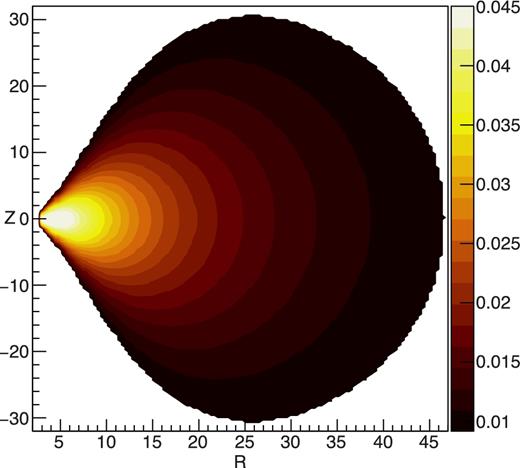
The temperature contours used for the simulation (for |$\dot{m}_{\rm d}=0.1$|, TCE = 25.0 keV, Xs = 46.8rS. The temperatures are written in dimensionless unit (kTe/mc2). This profile, symmetric with respect to z-axis, is used to get the values of temperatures at different points of CENBOL.
3.1.3 Keplerian disc (KD)
4 SCATTERING PROCESS
We adopt the method followed by Pozdnyakov, Sobol & Sunyaev (1983, hereafter PSS83) to model the thermal Compton scattering process.
4.1 Radiative processes
We continue the simulations for all the nine cases listed in Table 1. The angle θ*, number density nce and average temperature Te(τ0) were all derived from other parameters. Inclusion of the compression ratio (Rcomp) and mass of the star (MNS) would make the number of independent parameters to be seven. For our theoretical investigations in this paper, we did not focus on the reduction of the number of parameters in this work, but we can further reduce it by interrelating CENBOL properties from fundamental equations. We vary |$\dot{m}_{\rm d}$| and |$\dot{m}_{\rm h}$| independently and determine the rest of the parameters either using observational facts or through the formulae derived in Section 3. This has been discussed in Section 5.
4.2 Photoelectric absorption
In Figs 6–8, the dotted lines show our derived spectra before the interstellar absorption and solid lines show the spectra after absorption. For the cases C1–C9, nH = 4.0 × 1022 cm−2 was chosen for concreteness.
4.3 Effects of cooling
We focus on the cases when the CENBOL has temperature up to 25 keV, and the accretion rates are not too high (|${\le} \dot{M}_{{\rm Edd}}$|). In the flaring branches, however, the observed spectra show the Comptonized spectrum of to extend beyond 200 keV, pointing towards a hotter outer CENBOL. In order to check this effect of cooling, we take the case of comparatively hotter central temperature (TCE = 250 keV), and vary the accretion rates to observe the effects of cooling due to Comptonization. In the scenario when cooling is efficient, the static background temperature distribution should be modelled by the modified temperature, rather than the unmodified thick disc distribution. However, the spectra of those cases are not discussed any more as the Comptonized spectra of the disc is well understood in the cases of black hole under the TCAF paradigm.
We divide the CENBOL into two domains of equal optical depth, calculated along the equatorial plane. If the total optical depth of the CENBOL is τ0, the region up to τ = τ0/2 from the NBOL (or the shock location Xs) is the cloud ‘visible’ to the NBOL (or the KD), which would produce effectively the same number of scatterings. We determine the average temperature based on the method specified in equation (13), for both the cases, to study the effect of cooling of the CENBOL, by the NBOL and by the disc. This is just to find out the two temperatures in the two halves, which Seifina et al. (STF13, STSS15) and TSS14 found in their work by fitting COMPTB1 and COMPTB2, respectively. The results of this excercise is shown in Fig. 10(a)–(d).
5 RESULTS
The photons are collected outside a sphere of radius Rout where they leave our system. They are binned according to their energy, angle of observation, the original location of emission (NBOL or KD) and the number of scatterings each of them suffered. We generate the output spectra from these information.
We first report variation of spectra with respect to the number of scatterings in CENBOL. A considerable fraction of the seed photons emitted are intercepted by CENBOL. This interception and subsequent Comptonization depend on the density and temperature along the path of the photon. These parameters are, however, governed by the accretion rates. In case of a black hole, matter is advected in through the event horizon and the efficiency of radiation is around 6 per cent, leading to a large, though notional, upper limit (|$\sim\! 16\,\dot{M}_{{\rm EDD}}$|) of the KD accretion rate. In the case of an NS, the hard surface ensures the stopping of the flow at the surface and the radiation decreases the upper limit of maximum acceptable accretion rate. For our calculations, we have strictly kept the upper limit at |$1.0\ \dot{M}_{{\rm EDD}}$|. The density is, thus, lower than that around a black hole, leading to a lower number of scatterings of the photons emitted by the KD. The seed photons emitted by the NBOL, however, are exposed to the densest region of CENBOL first and that leads to a significant number of scattering. As a result, the contribution to hard X-Rays from seed photons that originated from the disc is smaller compared to those emitted from NBOL and the overall spectra, in hard states, is expected to be softer than the hard state spectra of a black hole. The observational differences are reported by Gilfanov (2010). We plot the variation of the combined spectra for the case C3 (from Table 1), with respect to the number of scattering in Fig. 3. The binning is done for scattering number 0 (no scattering), 1–2, 3–6, 7–18, 19–28, 29 and above. The overall spectra are also drawn. What is clear is that the photons from the KD are not scattered much. The lower number of scatterings (including those emitted without scattering) of NBOL photons produced the first hump at around 6 keV, while higher number of scatterings that are effectively close to the hot region of CENBOL (i.e. centre), produce the hump at ∼45 keV.
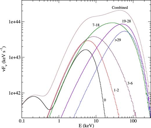
Evidence of hardening of spectra with the number of scattering. The seed photons are emitted from the NBOL and KD and are Comptonized by CENBOL. Here, halo accretion rate |$\dot{m}_{{\rm h}}$| is 0.5 and disc accretion rate is |$\dot{m}_{{\rm d}}$| is 0.1. The photons are binned based on the number of scatterings they underwent before emerging out of the system. The binning was done for 0, 1–2, 3–6, 7–18, 19–28, 29 or higher number of scatterings. These numbers are written beside the corresponding curves to give an idea of how variously scattered photons contribute to the spectra. The combined spectrum is also plotted.
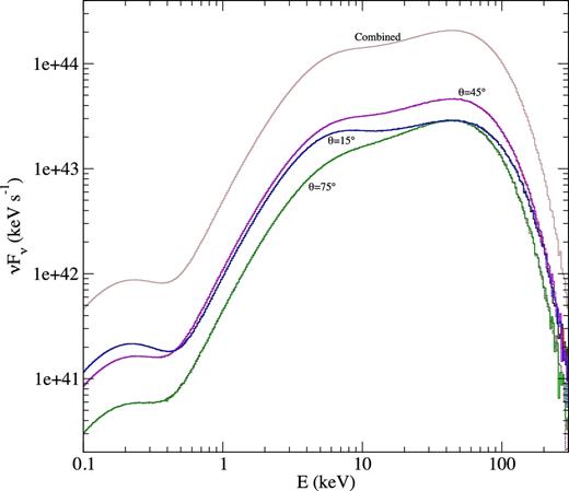
The spectral properties of any compact object in space, be it an NS or a black hole, depend on the inclination angle between the objects line of sight and direction in which the photon is emitted. In the presence of an accretion disc, which emits photons maximally along the local normal, the received flux is maximum when the disc is seen end-on and minimum when seen edge-on. In order to check the validity of any spectral model, it has to be compared with observational data and angle dependency of spectra is to be studied to achieve that. We plot the variation of spectra when the photons are binned with respect to the average direction of observation, viz., 0°–30°, 30°–60°, 60°–90°. In the system, both the photon sources emit photons symmetrically with respect to the equatorial plane or the angle θ = 90°. The structure of CENBOL has the same symmetry as well. As no advection velocity or spin effects are included to derive CENBOL properties, the emergent Comptonized spectra are expected to have the symmetry of the system. Thus in Fig. 4, we indicate the spectra of photons along the average bin angle in the bins of the first quadrant only. The peak flux of unscattered spectra from the KD decreases with increase of angle θ. In case of the radiation from NBOL, the peak flux direction is decided by the peaks of the double Gaussian distribution of emitted flux used in the simulation (Case C3) are along |$\theta _{\rm P}^-=54{^{\circ}_{.}}94$| in the first quadrant. The flux is modulated further due to the interception by CENBOL. The geometry of the post-shock region blocks the escape of unscattered photons emitted at high values of θ. This is reflected in Fig. 5(a). The low energy peaks are due to photons emitted from the KD and the high energy peaks are formed by photons from NBOL. The scattered photons, however, with the increase of the number of scatterings, lose their initial directional distribution and are re-distributed almost isotropically. Although, the presence of the disc and the NS, both of which recapture scattered photons, lowers the number of photons received at around angle θ = 90°. The net flux is highest at ∼45° since the flux of NBOL is high at |$\theta =\theta ^-_{\rm P}=54{^{\circ}_{.}}94$| and still has some direct effect. The remnant effect of the double Gaussian enhances the flux along this direction. The Fig. 5(b) showcases this.
Evidence of hardening of spectra with the observing angle. The seed photons are emitted from the NBOL and KD and are Comptonized by CENBOL. Here, halo accretion rate |$\dot{m}_{{\rm h}}$| is 0.5 and disc accretion rate is |$\dot{m}_{{\rm d}}$| is 0.1. Photons are binned according to the direction of observation. All the angles are measured with respect to the rotation axis (z-axis). The number beside each plot shows the corresponding average angle for each bin (°).
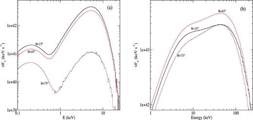
Evidence of hardening of spectra with the observing angle. The seed photons are emitted from the NBOL and KD and are Comptonized by CENBOL. The flow parameters are for Case C3 of Table 1. The photons are binned according to the direction of observation. All the angles are measured with respect to the rotation axis (z-axis). The numbers beside each plot shows the corresponding average angle bins (in degrees). In panel (a), only the photons that escape without being scattered are binned. The angle dependency arises out of the injection direction and geometry of CENBOL. In panel (b), all the photons that underwent at least one scattering are clubbed together.
As shown in the context of black holes (CT95; GCL09), a rise of halo accretion rate for a given disc accretion rate, makes the spectrum harder. Because of its hard surface, the upper limit of accretion rate for NSs is also much lower than that for black holes. This restricts the density of post-shock region leading to relatively softer spectra when compared to the spectra of black holes. Of course, a major factor is the abundance of seed photons from NBOL itself. Figs 6– 8 show how, in each case, the spectrum is affected by the increase of the halo accretion rate. In order to account for the cooling due to photons emitted by disc, we decreased the temperature of CENBOL self-consistently with the increase of |$\dot{m}_{\rm d}$| (see Table 1). In Fig. 8, the spectrum is roughly a superposition of two blackbody emissions in each of the three cases. In Fig. 7, the Compton up-scattering slightly modifies the spectra but they still remain in typical soft states. In Fig. 6, where TCE = 25 keV, the spectrum changes from soft to hard with the increase of |$\dot{m}_{\rm h}$|. We take the linear domain of the log (νFν) versus log (E) curves plotted in logarithmic scales, if present, and try to fit the data with a power law having spectral index α (νFν ∼ E−α). The spectral index α, has the values 0.926, 0.357 and −0.239 as |$\dot{m}_{\rm h}$| takes the values 0.1, 0.2 and 0.5, respectively. The indices are calculated from the best fit of the spectra in the energy range 10.0–20.0 keV. We have shown the theoretical spectra for cases C1–C9, in Figs 6–8, with dotted lines and the spectra after absorption through ISM are plotted with solid lines. Cases C1, C4, and C7 are in black, C2, C5, and C8 are in red and C3, C6 and C9 are in blue (online version). Please note that unlike some models (e.g. White et al. 1986; Mitsuda et al. 1989), we do not give emphasis on the NBOL temperature or the decrease of the total luminosity. Rather, our harder states are primarily achieved due to hotter CENBOL with higher advective halo rates.
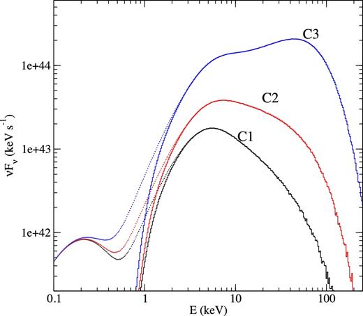
The variation of combined spectra from NBOL, KD and the Comptonized photons as |$\dot{m}_{{\rm h}}$| is varied from 0.1, 0.2 and 0.5. Here, |$\dot{m}_{\rm d}=0.1$| (Cases C1–C3). The dotted lines show our computed spectra as are emitted from the disc, while the solid lines show our spectra after absorption through ISM as they reach us. Here, we used photoelectric absorption due to hydrogen atoms, with nH = 4 × 1022 cm−2. The cases C1–C3 are shown in black, red and blue, respectively (online version).
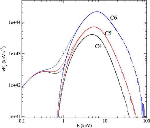
Variation of combined spectra from NBOL, KD and the Comptonized photons as |$\dot{m}_{{\rm h}}$| is varied from 0.1, 0.2 and 0.5. Here, |$\dot{m}_{\rm d}=0.2$|. (Cases C4–C6). Dotted lines show our computed spectra as are emitted from the disc, while the solid lines show our spectra after absorption through ISM as they reach us. Here, we used photoelectric absorption due to hydrogen atoms, with nH = 4 × 1022 cm−2. The cases C4–C6 are shown in black, red and blue, respectively (online version).
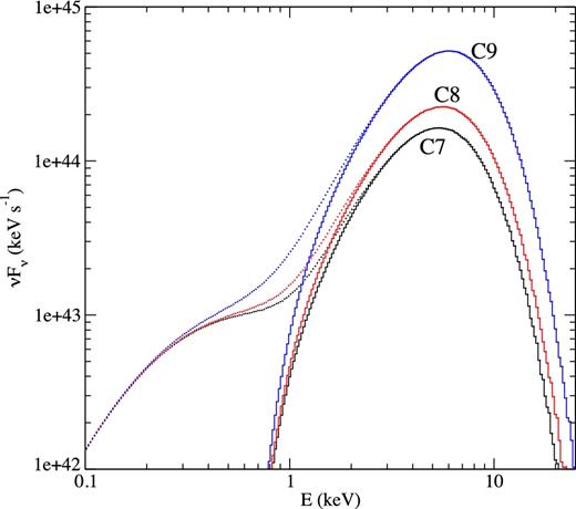
Variation of combined spectra from NBOL, KD and the Comptonized photons as |$\dot{m}_{{\rm h}}$| is varied from 0.1, 0.2 and 0.5. Here, |$\dot{m}_{\rm d}=0.5$|. (Cases C7–C9). Dotted lines show our computed spectra as are emitted from the disc, while the solid lines show our spectra after absorption through ISM as they reach us. Here, we used photoelectric absorption due to hydrogen atoms, with nH = 4 × 1022 cm−2. The cases C7–C9 are shown in black, red and blue, respectively (online version).
The absorption due to the presence of interstellar medium modifies the low energy spectra considerably. In the hard states, when the disc accretion rate is low, the multicolour blackbody component is hardly observed as a separate peak due to the heavy absorption below 1 keV. This was reflected in the Figs. 6–8. After these considerations, the spectra corresponding to Case C3, looks similar to hard state spectra of NSs (see fig. 9, adapted from Gilfanov 2010). The spectrum of NSs in hard states is relatively softer than those of black holes, because of the upper bound of maximum accretion rate. The spectra of a number of weakly magnetized accreting stars were chosen to highlight that fact in Fig. 9. They also have the characteristic iron line emission around 6.5 keV. Apart from that feature, the observed spectra of NSs, as reported in Gilfanov (2010), are similar to our Case C3, which does not include the iron line emission. It can also be concluded that the variation of the parameters of our model, for example, |$T_{{\rm NS}},\ T_{{\rm CE}},\ X_{\rm s},\ R_{{\rm comp}},\ \dot{m}_{\rm d}\ and\ \dot{m}_{\rm h}$| can reproduce the observed spectra when suitable normalization is used. In this paper, we report only the variation of spectra with accretion rates. The variation of other parameters and comparison with observed spectra would be reported elsewhere.
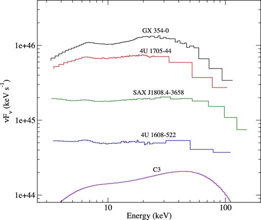
The spectra of a few weakly magnetized NSs, namely, 4U 1705-44, 4U 1608-522, SAX J1808.4-3658 and GX 354-0. For comparison, we put the spectrum of Case C3 (without the iron line emission) of our simulation to show that we generally reproduce the features. These observed spectra were obtained by RXTE observations and are adapted from Gilfanov (2010).
To check the variation of the effective geometry of the Compton cloud, CENBOL, as discussed in Section 4.3, we varied the accretion rates and the central temperature TCE of the CENBOL and observed how the Compton scattering changed the temperature profile. For TCE values reported in Table 1, the effect was insignificant and are not shown here. But, the cooling mechanism is more prominent when the central temperature is high. To showcase these effects, we chose the case where TCE = 250 keV and Xs = 46.8rS. We are reporting four cases here where the halo accretion rate is varied from 0.3 to 0.9, as shown in Fig. 10(a)–(d). As the accretion rates increase, so does the temperature of the NBOL, the cooling is more efficient. Not only that, the effective temperature closer to NBOL decreases more than the one nearer to the disc, as can be seen from the shifting of the peak towards the disc in Fig. 10(a)–(d). From these figures, one can see that the effective geometry of the CENBOL is similar to the ones proposed by TSS14 for the flaring branches. The temperature of cloud near the disc are in between ∼30 and ∼65 keV for the cases studied here, which are in the same ballpark figure as found from COMPTB model analysis in TSS14 and STSS15.
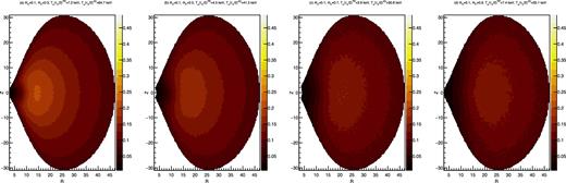
The temperature contours after Compton cooling, from the simulation (for initial TCE = 250.0 keV, Xs = 46.8rS). The temperatures are written in dimensionless unit (kTe/mc2). From the left- to right-hand side, the halo accretion rate is increased from 0.3 to 0.9. For panel (a)–(c), with the increase of |$\dot{m}_{\rm h}$|, the temperature of CENBOL closer to NBOL, Te(τ0/2)NS decreased from 7.2 to 3.6 keV. The temperature of CENBOL closer to disc, Te(τ0/2)KD, also decreased from 64.7 to 30.8 keV, but remain greater than the corresponding Te(τ0/2)NS. In the case of panel (d), where the angle θ* was π/2, a large fraction of blackbody photons escaped the system without scattering and hence the effect of cooling, although present, is less than the case panel (c). The modified contours show the effective region of Compton scattering and are similar to the proposed geometry of TSS14.
6 DISCUSSIONS AND CONCLUSIONS
In the literature, much studies have been done of the advective flows around black holes and their spectral properties. These solutions typically consist of two components, with a KD flanked vertically by an advective component. Moreover, the inner part of the advective component forms a centrifugal barrier and the post-barrier region (CENBOL) was found to behave as the Compton cloud producing typically the power law with exponential cut-off. CT95 has demonstrated that the spectrum changes from soft to hard as the relative importance of accretion rate of the Keplerian component vis-à-vis the accretion rate of the halo is decreased. Since the segregation of the advective flow into a Keplerian and sub-Keplerian components could take place very far out, there is no a priori reason why an NS accretion could not also manifest into the same two types of components, especially that very far away the flow has not knowledge of the nature of the compact object.
In this paper, we used the successful paradigm of TCAF in the context of a weakly magnetized NS accretion flow. The flow properties were changed on the NS surface due to modification of the inner boundary condition and a blackbody emitting NBOL is created on the NS surface, in addition to the CENBOL in TCAF. Due to the extra source of seed photons, the CENBOL became cooler easily and the spectra appeared to be softer for the same input flow parameters. The behaviour of CENBOL is similar to the Compton cloud invoked phenomenologically by TSS14. In our analysis, we restricted our studies within one Eddington rate. However, the general conclusion that the spectrum is hardened with the increase in halo accretion rate remains valid.
The resulting spectrum has several features arising out of the specific flux emission properties of the normal boundary layer, namely, NBOL. The radiation dynamics of NBOL with KD reveals (IS99) that the maximum flux emitted from the NBOL may not be really along the equatorial plane, but from an angle (θ*). This, together with the fact a CENBOL intercepts more photons from the NBOL than the Keplerian component, produces double hump patterns in the spectra. Photons from NBOL are inverse Comptonized more efficiently and thus dictate the spectra to a greater extent. We also studied how the spectra would change with the observing angle and found that with increasing inclination angle, the spectra are indeed hardened, a result also valid for black hole accretion (GCL09; GGCL10). However, unlike a black hole accretion, in the present scenario, the radiation could be maximum at an intermediate viewing angle (e.g. ∼45 in Fig. 4) and not necessarily along the polar axis.
The observed spectra from NS candidates, especially those which have weak magnetic fields, are found to have similar shapes as found in this paper thus confirming the general idea that TCAF can be used in the spectral study of NSs as well. For instance, the hard spectra of case C3 (Fig. 6) are similar to those of several NSs (Gilfanov 2010). Similar results have also been reported by Lin, Remillard & Homan (2007). Thus, the motivation of our exercise to check if the studies of the black hole and NS spectra could be carried out under a common framework is well justified.
Chakrabarti (1997) expanded CT95 work on TCAF to establish that the advective component of accretion (the sub-Keplerian halo) is essential to produce the hotter CENBOL. Otherwise, if the TL is produced solely from the KD and its optical depth and temperature were calculated self-consistently, the Comptonization would be sufficient to cool it down. Otherwise, one can use the latter quantities as free parameters without explicit use of the second component as in TSS14, who reproduce the spectra very satisfactorily. In this paper, we kept in mind the inter-relationship among the flow parameters and thus nine cases have been put in three main groups of increasing Keplerian accretion rate. Our NBOL cools the inner CENBOL rapidly. So in a way, the CENBOL behaves like the TL of TSS14.
It has been reported from observations that the photon index of COMPTB model for the νFν versus hν spectra reaches a saturation value of Γ ∼ 2, for the Comptonized spectra of an NS. The spectra from the disc's Comptonized components, however, show no such saturation in general. In ST11 and ST12, the spectra were fitted with Bbody + COMPTB + Gaussian, where the Bbody was related to the disc emission. In STF13, two COMPTB + Bbody components were used, where both the photon indices show stability around the value 2. In TSF13, the cloud temperature was seen to vary from 2.9 to 21 keV without any significant change in spectral slope of COMPTB spectra due to NS, but the normalization decreased by a factor of 8. TSS14 and STSS15 have shown the saturation of spectral index of COMPTB (for NS only) with respect to the variation of the temperature of the Compton cloud. The second COMPTB component showed a two-phase behaviour: In HB-NB, the photon index was around 2, but in FB, the photon index decreased and had values 1.3 < Γ < 2. It was stated that the spectrum at the FB is determined by high radiation pressure from the NS surface. Burke, Gilfanov & Sunyaev (2017) also reported the constancy of Comptonization parameters, which reflects saturation of photon index at around Γ ∼ 2. In all these cases, the illumination factor f, that controls the amount of Comptonization by the Compton cloud, underwent significant changes, which shows that the geometry or the size of the Compton cloud was changing with spectral states. In STS16, it was shown that the second COMPTB component (for the Comptonized spectra of the disc) showed variations around Γ ∼ 2. Γ went below 2 when the disc temperature is reduced from 1.1 to 0.8 keV, implying an expansion of Compton cloud. A simultaneous increase of the cloud temperature (of the outer part) was also observed. These phenomenological results can be very well understood by varying halo accretion rate, which appears to be the key controlling factor here. With the increase of |$\dot{m}_{\rm h}$|, more hot electrons are supplied, resulting in the expansion of CENBOL and spectral hardening (CT95, GGC14). We explore the variation of spectra with the halo accretion rate for such cases. The results are consistent with observed results.
The proposed geometry of the Compton cloud in TSS14, for the flaring branch shows a hotter outer TL and a cooler inner TL. When we consider the effects of cooling within the Monte Carlo simulation and modify the temperature of the CENBOL, a similar profile is obtained, as shown in Fig. 10(a)–(d). The peak of the distribution shifts towards the disc as accretion rate is increased, for a given initial set of temperature and shock location. The temperatures obtained by us are also consistent with the observed values as reported in TSS14 and STSS15.
Recently, the TCAF solution has been used to fit spectra of several black hole candidates and at the same time to extract physical flow properties and the mass of the compact object (Molla et al. 2017, 2016; Bhattacharjee et al. 2017, and references therein). In near future, we plan to extract physical flow parameters on to NSs as well. Similarly, we are also extending the time-dependent studies of TCAF flow with radiative transfer in order to understand real reason for the high and low-frequency quasi-periodic oscillations in NS systems. In a future work, we will compare the spectral fits using our model and fits obtained using COMPTB model.
Acknowledgements
We would like to the thank the referee Dr Lev Titarchuk for bringing to our attention the Comptonizing properties of their TL.
REFERENCES
