


Abstract
The X-ray variability of the BL Lacertae source 1ES 1959+650 was studied intensively with X-ray telescope (XRT) onboard Swift during 2016 January–August. In this paper, we present the results obtained during this campaign. A long-term high X-ray state was superimposed by shorter-term flares by a factor of 1.9–4.7. We found 35 instances of intra-day variability which showed very fast flux changes by 14–21 per cent occurring within 1 ks and a decline by a factor of 2.3 in 17.2 ks. Similarly to the previous years, this period sometimes was characterized by a lack of correlated X-ray and TeV variability, indicating that the high-energy emission in 1ES 1959+650 was generated in the emission region more complex than a single zone. The source showed a significant X-ray – high-energy flux correlation, while the former was not correlated with the optical–UV fluxes. The best fits of the 0.3–10 keV spectra were mainly obtained using the log-parabola model. Strong spectral variability was detected, shifting the peak of the spectral energy distribution by more than 10 keV that happens rarely in blazars. During some strong short-term flares, the photon index at 1 keV frequently became harder than 1.70, and the spectral evolution was characterized by a harder-when-brighter behaviour.
1 INTRODUCTION
Blazars (BL Lacertae objects and Flat Spectrum Radio Quasars) constitute an extreme class active galactic nuclei (AGNs) with a broad continuum extending from the radio to the very high-energy (VHE, E >100 GeV) γ-rays, representing a majority of TeV-detected extragalactic sources.1 They also exhibit double-humped spectral energy distribution (SED), compact radio emission and superluminal motion of some components (Falomo, Pian & Treves 2014). These features are explained as a non-thermal emission from the relativistic jet closely aligned to our line of sight (Blandford & Rees 1978 and references therein).
Moreover, BL Lacertae objects (BLLs) are also prominent with weak or absent emission lines and strong, rapid variability in different spectral bands. Due to the observed high optical and radio polarization, the lower energy SED component is firmly attributed to synchrotron radiation emitted by ultrarelativistic electrons in the jet. Based on the location of the synchrotron SED peak Ep, BLLs are broadly divided into ‘low-energy-peaked BLLs’ (LBLs, with Ep situated in the IR-optical range) and ‘high-energy-peaked BLLs’ (HBLs, with Ep observed at UV-X-ray frequencies; see Padovani & Giommi 1995). However, there is a variety of the models explaining the origin of the higher-energy ‘hump’: an inverse Compton (IC) scattering of synchrotron photons by the same electron population (synchrotron self-Compton, SSC; Marscher & Gear 1985 and references therein), ambient photons scattered by the jet particles (external Compton; Dermer, Schlickeiser & Mastichiadis 1992) and hadronic processes (e.g. Mannheim 1993).
An intense multiwavelength (MWL) flux variability and inter-band cross-correlation study of different BLLs allows us to discern a valid emission model for the higher energy component, underlying physical processes, unstable processes triggering the observed flux and spectral changes. Moreover, X-ray spectral analysis is a powerful tool for revealing the distribution of emitting particles with energy and draw conclusions about the extreme processes accelerating them up to tremendous energies. X-ray telescope (XRT; Burrows et al. 2005) onboard Swift Gehrels et al. (2004) is optimal to accomplish the aforementioned tasks due to its low background counts, unique instrumental characteristics and good photon statistics. The same properties allow us to search for the flux variability on diverse time-scales, derive the values of different spectral parameters with a high accuracy and to study their timing behaviour.
In this paper, we report the results of MWL observations of the nearby (z = 0.048; Perlman et al. 1996) TeV-detected HBL source 1ES 1959+650 based on the intensive Swift observations performed during 2016 January–August which followed the strong and prolonged X-ray flaring activity of this source in 2015 August–2016 January (Kapanadze et al. 2016a; hereafter Paper I). The majority of these observations were performed in the framework of our target of opportunity (ToO) observations of different urgencies which allowed us to obtain densely sampled X-ray, UV and optical light curves in one of the most important epoch since the detection of our target within Einstein Slew Survey (Elvis et al. 1992). First, we concentrate on the 0.3–10 keV band observations performed with XRT. Along with these data, we have analysed those obtained with the Ultraviolet-Optical Telescope (UVOT; Roming et al. 2005) and the Burst Alert Telescope (BAT; Barthelmy et al. 2005) onboard Swift to draw conclusions about the target's long-term MWL behaviour and search for inter-band correlations. For these purposes, we also included the results from other MWL observations performed in the VHE, high-energy (HE, E > 1 MeV), optical (R and V bands) and at the 15 GHz frequency obtained with First G-APD Cherenkov Telescope (FACT; Anderhub et al. 2013), Large Area Telescope (LAT) onboard Fermi Atwood et al. 2009), different Earth-based telescopes, and OVRO 40-m telescope (Richards et al. 2011), respectively. We re-consider the results from Paper I to compare them with those obtained here.
The paper is organized as follows. Section 2 describes the data processing and analysis procedures. In Section 3, we provide the results of a timing and spectral analysis. We discuss our results in Section 4, and provide our conclusions in Section 5.
2 OBSERVATIONS AND DATA REDUCTION
2.1 X-ray, UV and optical observations
The source was observed 69 times with XRT in the 0.3–10 keV energy range between 2016 January 21 and August 12 with a total exposure of 75 ks. The information about each pointing are provided in Table 1.2 The unscreened event files from the XRT observations were reduced, calibrated and cleaned with the script xrtpipeline (operating within xrtdas software which is a part of heasoft v.6.213) using the standard filtering criteria and the latest calibration files of Swift CALDB v.20170501. We selected the events with the 0–2 grades for the Windowed Timing (WT) mode, whereas the range of 0–12 was used for the Photon Counting (PC) observations. The latter mode was used only on two occasions in the period presented here (ObsID 00035025247 and 00035025255). The selection of the source and background extraction regions, as well the correction of the source's count rates on a pile-up and other effects (bad/hot pixels, vignetting) were done within xselect, following the standard procedure described in detail by Kapanadze et al. (2016b, hereafter K16b). The background-subtracted light curves were constructed using various time bins (see Section 3.1.4).
XRT observations of 1ES 1959+650 in 2016 January–August (extract). The columns are as follows: (1) – observation ID; (2)– observation start and end (in UTC); (3) – exposure (in seconds); (4) – Modified Julian date corresponding to the observation start; (5)–(8): mean count rate with its error (in cts s−1), reduced χ2, presence of a variability (‘V’: variable; ‘PV’: possibly variable; ‘NV’: non-variable), respectively.
| ObsID | Obs. start–end (UTC) | Exposure (s) | MJD | Flux (cts s−1) | χ2/d.o.f. | Bin (s) | Var. |
|---|---|---|---|---|---|---|---|
| (1) | (2) | (3) | (4) | (5) | (6) | (7) | (8) |
| 00035025208 | 2016-01-21 23:58:58 01-22 01:02:53 | 716 | 57409.004 | 8.91(0.13) | 1.524/9 | 60 | NV |
| 00035025209 | 2016-01-26 13:55:57 01-26 19:47:13 | 1839 | 57413.583 | 3.23(0.05) | 18.94/2 | Orbit | V |
| 00035025210 | 2016-01-29 13:38:57 01-29 14:40:15 | 629 | 57416.570 | 3.80(0.08) | 1.09/8 | 60 | NV |
| 00035025211 | 2016-02-09 13:24:59 02-09 22:27:57 | 1595 | 57427.561 | 7.08(0.07) | 1.149/25 | 60 | NV |
From the publicly available 1-week binned light curves of 1ES 1959+650 obtained with MAXI,4 we used only those data corresponding to the source's detection with 5σ significance for a flux variability study. The BAT data, taken from the Swift-BAT Hard X-ray Transient Monitor program5 (Krimm et al. 2013), have been re-binned with the tool REBINGAUSSLC (included in heasoft) using the time bins of 1–4 weeks.
The source was observed with UVOT telescope (a Ritchey–Chrétien system with 30-cm mirror; Roming et al. 2005) in the six photometric bands UVW2, UVM2, UVW1, U, B and V simultaneously with those of the XRT, covering the wavelength range of 1700–6600 Å. Using the sky-corrected images, maintained by HEASARC,6 the photometry was performed using the UVOTSOURCE tool with the apertures with the radii of 5 and 10 arcsec for the optical and UV bands, respectively. The derived magnitudes were corrected for the Galactic absorption and converted into milli-Janskys according to the recipe provided by K16b (see Table 2 for the results).
The results of the UVOT observations (extract). The flux values in each band are given in units of mJy.
| V | B | U | UVW1 | UVM2 | UVW2 | |||||||
|---|---|---|---|---|---|---|---|---|---|---|---|---|
| ObsId | Mag. | Flux | Mag. | Flux | Mag. | Flux | Mag. | Flux | Mag. | Flux | Mag. | Flux |
| 35025208 | 14.13(0.05) | 8.17(0.35) | 14.46(0.04) | 6.67(0.19) | 13.51(0.04) | 5.70(0.20) | 13.41(0.04) | 3.84(0.17) | 13.24(0.04) | 3.87(0.11) | 13.24(0.04) | 3.73(0.14) |
| 35025209 | 14.23(0.06) | 7.45(0.39) | 14.59(0.04) | 5.92(0.23) | 13.78(0.04) | 4.45(0.18) | 13.64(0.04) | 3.10(0.15) | 13.57(0.06) | 2.86(0.15) | 13.44(0.05) | 3.10(0.14) |
| 35025210 | 14.14(0.05) | 8.09(0.38) | 14.58(0.04) | 5.97(0.21) | 13.61(0.04) | 5.20(0.20) | 13.53(0.05) | 3.44(0.15) | 13.37(0.05) | 3.44(0.15) | 13.40(0.04) | 3.22(0.14) |
| 35025211 | 14.05(0.06) | 8.79(0.45) | 14.54(0.05) | 6.19(0.26) | 13.59(0.04) | 5.30(0.24) | 13.47(0.05) | 3.63(0.19) | 13.26(0.05) | 3.80(0.15) | 13.34(0.05) | 3.40(0.14) |
2.2 γ-ray observations
Since 2005 August, 1ES 1959+650 has been monitored with Fermi–LAT in the sky-survey mode. Although this instrument is sensitive in the range from 20 MeV to more than 300 GeV,7 we used only the photons with the energy of 300 MeV–100 GeV due to two reasons: (i) the effective area of the instrument is relatively large (>0.5 m2) and the angular resolution relatively good (the 68 per cent containment angle smaller than 2 deg) at the energies above 0.3 GeV (Atwood et al. 2009). Consequently, the spectral fit is less sensitive to possible contamination from unaccounted, transient neighbouring γ-ray sources and we obtain smaller systematic errors (Abdo et al. 2011); (ii) to compare our results to those presented in Aliu et al. 2013 and Kapanadze et al. 2016a,b, using the same energy range.
The analysis was performed with the software package fermi science tools version 10r0p5 with the instrument's response function P8R2_V6. We extracted the 0.3–100 GeV photon flux from a region of interest (ROI) with the 10 deg radius centred at the location of 1ES 1959+650, computed its detection significance and derived the values of spectral parameters using the unbinned likelihood analysis method GTLIKE.8 The data screening criteria were as follows: (1) only the events of the ‘diffuse’ class, i.e. those with the highest probability of being photons are included in our analysis; (2) the data corresponding to the satellite's ‘rocking’ angle larger than 52 deg are discarded to avoid contamination from photons from the Earth's limb; (3) a cut on the zenith angle (>100 deg) was applied to reduce contamination from the Earth-albedo γ-rays, generated by the cosmic rays interacting with the upper atmosphere.
For the spectral analysis, we generated a background model (an XML file) including: (i) all γ-ray sources from the Fermi-LAT 4-yr Point Source Catalog (3FGL, Acero et al. 2015) within 20 deg of 1ES 1959+650. The spectral parameters of sources within the ROI were left free during the minimization process, and those outside of this range fixed to the 3FGL catalogue values; (ii) a Galactic diffuse emission component by applying the recommended model file gll_iem_v06.fits; (iii) the isotropic component, representing the sum of the extragalactic diffuse emission and the residual charged-particle background. It was parametrized with a single power-law function. The photon index of the isotropic component and the normalization of both components in were allowed us to vary freely during the spectral point fitting to reduce systematic uncertainties in the analysis.
For the spectral modelling of 1ES 1959+650, we adopted a simple power law, similar to the 3FGL catalogue. We used the 3-d binned data to construct the 0.3–100 GeV light curve corresponding to 2015 August 1–2017 August 12, since the source was significantly brighter and showed higher detection significances than in the previous 7-yr period of the LAT monitoring (see Section 3.1.2). Therefore, we adopted 2-weekly binned data for the construction of the historical LAT-band light curve to warrant the target's detection with 3σ significance.
1ES 1959+650 is one of the sources regularly monitored at TeV energies with the imaging air Cherenkov telescope FACT located at Observatorio del Roque de los Muchachos (La Palma, Spain) and operational since 2011 October. Since 2012 December, the results of a preliminary quick-look analysis are published immediately or with a short latency at the corresponding website.9 These background-subtracted light curves are constructed on the basis of the excess rates from 1ES 1959+650 which have not been corrected for the effect of changing energy threshold related to the variations in the zenith distance and ambient light, and no data selection is done (see Dorner et al. 2015 for the details of the quick look analysis). Totally, more than 300 h of data are available for 1ES 1959+650 from the FACT quick-look analysis between 2012 December and 2016 August. In our study, we have restricted the sample to the nights with a signal detected with a minimum significance of 3 σ. From the daily binned FACT data of 1ES 1959+650, we used 47 nights (142 h) for our study in 2016 and 53 nights (155 h) in total. All of these data are taken under light conditions with a stable energy threshold and more than 86 per cent have a zenith distance not changing the energy threshold. The nightly observation time was between 0.5 and 4.4 h.
3 RESULTS
3.1 Flux variability
3.1.1 Long-term X-ray variability
Fig. 1(a) presents the historical light curve of 1ES 1959+650 from the XRT observations which shows that the source exhibited another strong prolonged X-ray flaring activity after that presented in Paper I (2015 August 1–2016 January 19; hereafter ‘Period 1’). The source showed the highest historical 0.3–10 keV count rate of 24.78 ± 0.25 cts s−1 on 2016 July 2 (MJD 57571.24) that is 15 per cent larger than the previous highest value recorded on 2015 December 26 (MJD 57392.75; Period 1; see Fig. 2a). Moreover, the weighted mean rate from the observations in 2016 June 4–August 3, when the source was most active (hereafter ‘Period 3’), amounts to 15.25 ± 0.03 versus 9.72 ± 0.02 cts s−1 in Period 1. If we exclude the XRT observations performed in 2015 August–2016 August, those from the pervious 10.35 yr period yielded the weighted mean rate |$\overline{CR}_{\rm 2005-2015}$| = 5.91±0.01 cts s−1, i.e. the aforementioned 1 yr period was the epoch of strongest X-ray activity of our target since the start of Swift observations. However, these two strongest X-ray flares were separated by the period of a relatively modest flaring behaviour (2016 January–May; ‘Period 2’) with the maximum-to-minimum flux ratio R = 4.19, and the maximum 0.3–10 keV count rate of 13.54 ± 0.13 cts s−1. The latter is smaller than the maximum rate observed during the X-ray flare in 2006 (see Kapanadze et al. 2016b).
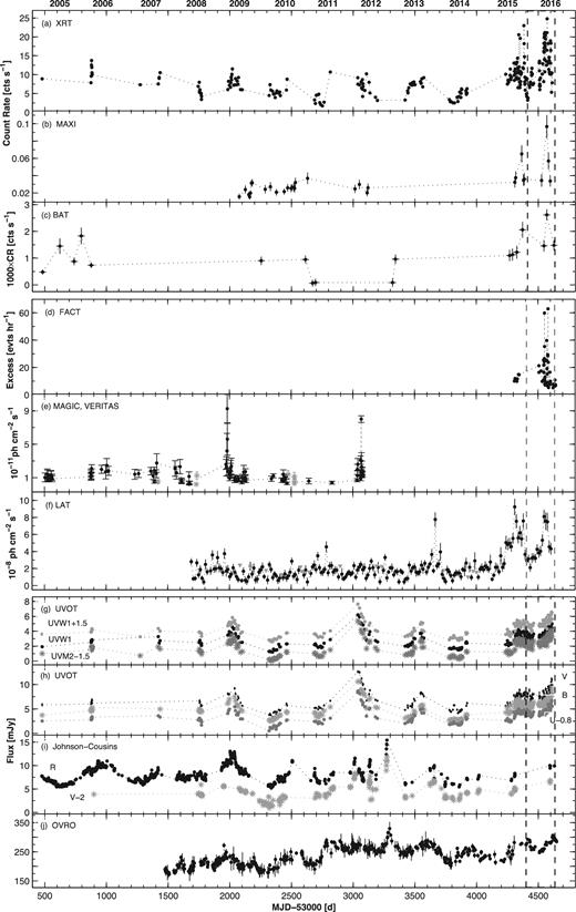
The historical light curves of 1ES 1959+650 from the MWL observations in 2005–2016 with XRT (top panel), MAXI (panel b), BAT (panel c), FACT (panel d), MAGIC and VERITAS (panel e), Fermi–LAT (panel f), UVOT (panels g and h), ground-based telescopes (panel i) and OVRO (panel j). We used daily bins for XRT, BAT, FACT, UVOT, Steward, OVRO data; 1 2 and 4-week bins for those of MAXI, LAT and BAT observations, respectively. The light curves between the vertical dashed lines correspond to the period 2016 January–August.
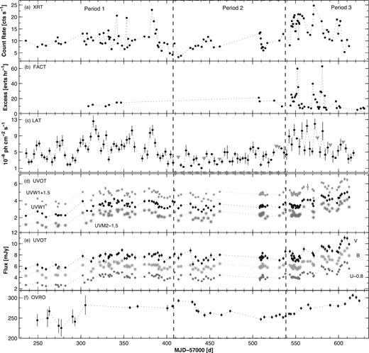
MWL variability of 1ES 1959+650 in Periods 1–3 (with the same time bins used in Fig. 1, except for the LAT data binned within 3 d intervals). Grey triangles in panel c stand for 2σ upper limits to the LAT flux when the source was detected below the 3σ significance.
In 2009–2016, 1ES 1959+650 was detected 31 times in the 2–20 keV band with 5σ significance from the weekly binned MAXI observations, and the maximum-to-minimum flux ratio R = 6.26. The historical 2–20 keV light curve shows two prominent flares in Periods 1 and 3, and the corresponding maximum count rates are a factor of 2–3 larger than the maximum rate from the previous detections in 2009–2012 (Fig. 1b). The MAXI observations of 1ES 1959+650 also show that the source underwent a stronger X-ray flare in Period 3 and the peak flux was 50 per cent larger than in Period 1. Similar results are obtained from the BAT observations, although the source generally is very faint in this band, and it was detected only 18 times with 5σ significance from the 4-week binned data (Fig. 1c). These detections show a very broad range of 15–150 keV count rate with R = 41.5, and we observe two prominent peaks in Periods 1 and 3, respectively, which are 13–42 per cent higher than that in the epoch of the X-ray flare in 2006.
3.1.2 Long-term variability in other spectral bands
The source was detected above the 3σ significance 35 times in Period 3 from the daily-binned FACT data, while it was detected only 6 and 4 times in Periods 1 and 2, respectively (although there was a long interruption in the FACT observations in Periods 1 and 2 during MJD 57367–57506 due to the visibility reasons of the source; see Fig. 2b), and there is no detection for a nightly binning before 2015 October since the start of the FACT observations of our target (2012 December 13; Fig. 1d). While these rare detections do not show a significant variability in Periods 1 and 2, three strong flares by a factor of 5.55–9.50 were evident in Period 3 (see also Dorner et al. 2016; Biland et al. 2016a,b,c). From the 20-min binned FACT data, the source was detected above the 3σ significance 73 times in Period 3 (90 per cent of all detections in 2013–2016) with the maximum-to-minimum flux ratio R = 5.85.10
The source mostly was faint in the 0.3–100 GeV band, and we used 2-week bins for the construction of the corresponding historical light curve that yielded the detection above the 3σ threshold except for the 13 occasions which occurred during 2009–2014 (see Fig. 1f). The latter exhibits two prominent long-term flares by a factor of 3.9–8.5 coinciding with Periods 1–3, while no clear, strong long-term flares are evident from the observations of the previous years, and there is only a fast strong ‘flash’ by a factor of 4.5 around MJD 56667 (2014 January). The source was always detectable from the 3 d binned LAT data above the 3σ threshold in Period 1 or mostly detectable in Periods 2 and 3 (Fig. 2c), while a detection with the 3 d binning was rare from the observations performed in 2008 August–2015 July. Nevertheless, 22.6 per cent of the 1 week bins in this period show a detection below the 3σ threshold that happened only once during Period 1–3 (in 2016 February). The mean 0.3–100 GeV flux in Periods 1–3 amounted to (4.35 ± 0.13) × 10−8 photons cm−2 s−1, while this value was a factor of 2.85 smaller for the whole previous 7 yr period. In the case of the 3 d binning, the 0.3–100 GeV flux varied by a factor of 11.5 during 2016 January–August, and exceeded the threshold of 10−7ph cm−2 s−1 five times in Period 3.
The source showed a significantly weaker and slower variability with the maximum-to-minimum flux ratio R = 1.86–2.07 in the UVW1, UVM2 and UVW2 bands compared to the X-ray–TeV energy range (Fig. 2d). In many cases, the source did not undergo an enhanced UV activity, and sometimes it showed a decreasing trend or even a minimum along with strong X-ray flares. The highest UV state in the presented period was observed in the early August (at about MJD 57607), in contrast to the higher energy bands, and 2016 January–August was not the period of highest historical UV fluxes which were recorded in 2012 May (MJD∼56050; see Fig. 1g). A similar behaviour is also evident in the UVOT optical V, B, U bands (Figs 1h and 2g), where the variability is even smaller with R = 1.74–1.87. This is partially explained by the significant contribution from the bright host galaxy than in the UVW1–UVW2 bands. Fig. 1(i) presents the historical light curves in the V and R bands of the Johnson–Cousins system, constructed via the data provided in Kapanadze et al. (2016b), Yuan, Fan & Pan (2015) and presented at the website the Steward observatory.11 They exhibit the highest optical states around MJD 56273 when the Swift observations were not carried out, and very few V and R band data are available in the period presented here. In these bands, we observe larger maximum-to-minimum flux ratios (R = 2.97–4.69) than in the UVOT bands. This can be related to the densely sampled V and R band data and the presence of ground-based observations in some epochs when no UVOT observations of 1ES 1959+650 were carried out.
Finally, the 15 GHz data obtained with the OVRO 40-m telescope in the period 2016 January–August exhibit a significantly slower and weaker variability with R = 1.24 than in other spectral bands (Fig. 2f). In Period 3, the source showed a long-term brightening by 22 per cent, and the radio light curve exhibits its maximum with ∼1 week delay with respect to the optical–UV maxima. The historical light curve also shows a slow variability with R = 1.91 (Fig. 1j). Note that the highest historical radio state of 1ES 1959+650 at MJD ∼ 56300 (the end of 2012 and the start of 2013) nearly coincided with that recorded in the V and R bands (with a delay by about 2 weeks).
3.1.3 Shorter-term flares
Below, we concentrate on the detailed results from Periods 2 and 3 and their particular parts (selected according to the occurrence of short-term flares in the XRT band) whose summary is presented in Table 3. For each period or sub-period, the fractional variability amplitude and its error is calculated according to Vaughan et al. (2003) and reported in this table. The MWL light curves from each sub-period are provided in Fig. 3. For comparison, Table 3 also contains the results from Period 1 (see Paper I for its detailed description).
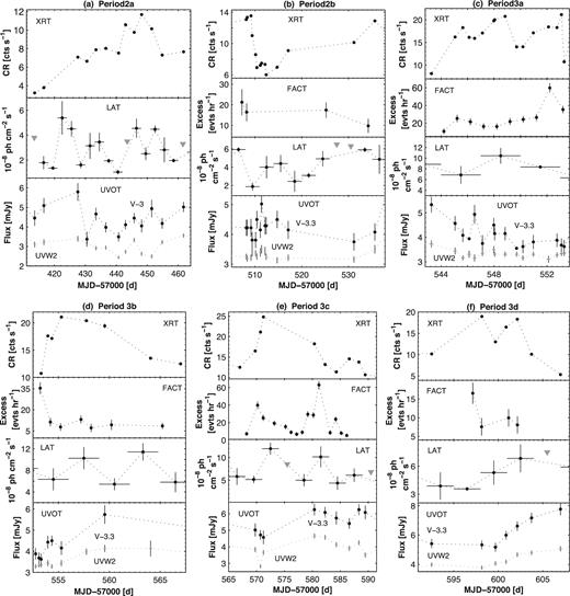
Multiwavelength variability of 1ES 1959+650 in different sub-periods. Grey triangles in panel b stand for upper limits to the LAT flux when the source was detected below the 3σ significance.
Summary of the XRT, UVOT, LAT and FACT observations in different periods. Col. 3–5: maximum 0.3–10 keV flux in cts s−1), maximum-to-minimum flux ratio and fractional amplitude (per cent) in each period, respectively; Col. 6–9: maximum values (in 10−11 erg cm−2s−1) and maximum-to-minimum flux ratios for unabsorbed 0.3–2 keV and 2–10 keV fluxes; Col. 10–14: maximum-to-minimum flux ratios in the UVOT bands, and those from the LAT and FACT observations in columns 16–17.
| XRT | UVOT | LAT | FACT | |||||||||||||
|---|---|---|---|---|---|---|---|---|---|---|---|---|---|---|---|---|
| Per. | Dates | CRmax | R | Fvar | |$F^{\text{max}}_{2-10}$| | R2–10 | |$F^{\text{max}}_{0.3-2}$| | R0.3–2 | RUVW2 | RUVM2 | RUVW1 | RU | RB | RV | R | R |
| (1) | (2) | (3) | (4) | (5) | (6) | (7) | (8) | (9) | (10) | (11) | (12) | (13) | (14) | (15) | (16) | (17) |
| 1 | 2015 August 1–2016 January 19 | 22.97(0.16) | 5.51 | 34.6(0.2) | 50.58 | 8.20 | 34.67 | 3.10 | 2.22 | 2.01 | 2.03 | 1.86 | 1.77 | 1.63 | 6.52 | 1.51 |
| 2 | 2016 January 21–May 27 | 13.54(0.13) | 4.19 | 30.4(0.2) | 27.86 | 8.49 | 30.55 | 3.69 | 1.63 | 1.54 | 1.40 | 1.32 | 1.31 | 1.38 | 6.21 | 2.18 |
| 2a | 2016 January 26–March 14 | 11.67(0.11) | 3.61 | 31.2(0.3) | 18.79 | 5.73 | 26.98 | 3.26 | 1.46 | 1.46 | 1.34 | 1.28 | 1.31 | 1.38 | 5.18 | – |
| 2b | 2016 April 30–May 27 | 13.54(0.13) | 2.25 | 28.8(0.3) | 27.86 | 3.09 | 30.55 | 2.12 | 1.27 | 1.35 | 1.19 | 1.25 | 1.14 | 1.22 | 3.17 | 2.18 |
| 3 | 2016 June 4–August 12 | 24.78(0.25) | 4.66 | 25.9(0.2) | 55.59 | 12.59 | 49.43 | 3.96 | 1.80 | 1.62 | 1.56 | 1.65 | 1.61 | 1.62 | 3.60 | 11.98 |
| 3a | 2016 June 4–June 14 | 21.13(0.17) | 2.60 | 21.3(0.2) | 52.24 | 4.52 | 43.75 | 3.51 | 1.20 | 1.20 | 1.16 | 1.16 | 1.15 | 1.26 | 1.65 | 5.50 |
| 3b | 2016 June 14–June 27 | 21.07(0.12) | 1.96 | 23.3(0.5) | 52.48 | 2.00 | 42.66 | 1.51 | 1.26 | 1.28 | 1.27 | 1.25 | 1.21 | 1.31 | 2.10 | 1.84 |
| 3c | 2016 June 27–July 20 | 24.78(0.25) | 2.32 | 28.9(0.4) | 55.59 | 3.24 | 49.43 | 2.17 | 1.66 | 1.53 | 1.37 | 1.37 | 1.25 | 1.21 | 2.74 | 11.98 |
| 3d | 2016 July 23–August 6 | 18.95(0.12) | 3.56 | 38.0(0.3) | 38.55 | 8.73 | 37.84 | 2.92 | 1.34 | 1.29 | 1.31 | 1.41 | 1.35 | 1.31 | 1.92 | 2.19 |
In the beginning of Period 2 (denoted as Period 2a; see Table 3), the source underwent an X-ray flare by a factor of 3.6 in 35 d (Fig. 3a, top panel). In the epoch of the highest X-ray state, the source also showed an enhanced activity in the 0.3–100 GeV band (second panel). Moreover, the largest LAT-band flux was observed around MJD 57522 when the source showed a short-term γ-ray flare by a factor of 4 (with no contemporaneous XRT observations). Although the UVOT-band fluxes showed an increase by 10–25 per cent after the start of the X-ray flare, they exhibited a decline after MJD 57427.6 until the lowest optical–UV state during the whole 2016 January–August period (bottom panel).
The highest 0.3–10 keV state in the whole Period 2 was recorded in the initial part of Period 2b (see Table 3 and Fig. 3b), followed by a fast decline by a factor of 2.25 in 3 d and by a subsequent slow increase by a factor of 2.15 in about 3 weeks. A nearly similar behaviour was observed in the 0.3–100 GeV band. The optical–UV fluxes did not exhibit any correlation with their X-ray–HE counterparts (bottom panel), and reached their maximum values in this sub-period on MJD 57511 when the source was in its lowest X-ray state. 1ES 1959+650 was detected by FACT four times with 3σ significance in this sub-period, and the VHE flux also do not show a correlated variability with the 0.3–10 keV one.
We observe a fast X-ray flare by a factor of 2.25 in 2.3 d in the beginning of Period 3a (see Table 3 and Fig. 3c), and, afterwards, superposed on the longer-term flux variability were two minor flares whose light curves were similar to each other: a relatively slow brightness increase by 30–50 per cent in 2.3–2.9d, and the peaks of the corresponding light curves were followed by a significantly faster drop by 34 per cent in 1.5 d and by a flux halving in 4.7 h for the first and second flares, respectively. Note that the similar declines occurred very fast also during the most active phases of a strong X-ray flares in Period 1 (decays by a factor of 2.3–2.7 in 0.75–1.05 d on MJD 57342 and 57352, respectively; see Fig. 3a and Paper I). The FACT light curved exhibits the first, relatively low peak on MJD 57545 and subsequent decline, similar to the 0.3–10 keV one. The second, significantly stronger VHE flare occurred in the epoch of the aforementioned second minor X-ray flare. However, the source did not show an enhanced VHE flux around MJD 57550 when the XRT and LAT-band peaks were observed. As for the optical–UV light curves, they show the highest fluxes at the start of Period 3a (coinciding with the minimum of the 0.3–10 keV flux), followed by a decline along with X-ray flares.
The 0.3–10 keV and VHE fluxes showed an opposite behaviour in Period 3b (see Table 3 and Fig. 3d): while the source was detected above the 20 cts s−1 level after a fast brightening by 96 per cent in 2 d, and the FACT light curve exhibits a brightness drop by a factor of 5.1, although it could be related to the worsened observational conditions (the presence of the Moon and Calima). The first LAT-band peak coincided a high X-ray state, while the second one was not accompanied by enhanced X-ray flux. A similar situation was also observed in Period 3c (see Table 3 and Fig. 3e): The first LAT-band peak was observed in the epoch of the highest historical 0.3–10 keV flux (recorded on MJD 57571 after the doubling in X-ray flux in 4.3 d, accompanied by a VHE flare by a factor of 5.6), while the second one occurred in the epoch of decreasing X-ray flux. Note that the latter peak coincided with a strong VHE flare by a factor of 7.1. However, XRT observed 1ES 1959+650 only twice during this event, and we cannot draw a firm conclusion about the lack of the VHE–X-ray correlation. The subsequent, low VHE peak was observed on MJD 57585 when the 0.3–10 keV light curve exhibited its minimum.
As for Period 3d (see Table 3), the source underwent a short-term X-ray flare with two peaks in the high brightness epoch (accompanied by a low VHE state), and the second one was accompanied by a peak in the 0.3–300 GeV light curve (Fig. 3f). Similar to Period 3b, we observe low UVOT-band fluxes during a high X-ray state and an optical–UV brightening along with the declining 0.3–10 keV flux.
3.1.4 Intra-day variability
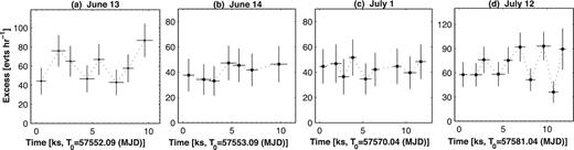
We detected 35 instances of intra-day variability (IDV, a flux change within a day; Gupta et al. 2012) of the 0.3–10 keV flux during 2016 January–August at the 99.9 per cent confidence level, by applying the χ2-statistics. Table 4 presents fractional variability amplitude, ranges of the spectral parameters a (or Γ), b, Ep and HR for each event. The fastest variability was recorded on June 15 (MJD 57554) when the 0.3–10 keV flux showed an increase and subsequent decline by about 20 per cent within 420 s, followed by the next increase by 14 per cent in 240 s during the first orbit of ObsID 00034588003 (Fig. 4a). This instance corresponded to one of the brightest X-ray state of the source. Another very fast IDV was recorded on May 9 (MJD 57517.2) when the brightness decreased by 20 per cent in 600 s (Fig. 4b). The source exhibited very fast variability with a decline by 21 per cent within 600 s on May 4 (MJD 57517.4; see Fig. 4c). Although we observe a significantly faster decline in the beginning of this observation, it could be related to the instrumental effects. The source had undergone a very fast increase by 16 per cent 750 s before reaching its highest historical 0.3–10 keV brightness state on July 2 (MJD 57571; Fig. 4d), and exhibited a fast fluctuation by about 15 per cent within 600 s on June 6 (during ObsID 00035025231; Fig. 4e). The strongest IDV was recorded on June 13–14 (MJD 55552) when the brightness dropped by a factor of 2.3 in 17.2 ks (Fig. 4f).
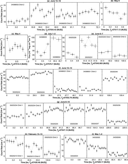
The most notable X-ray IDVs of 1ES 1959+650 in 2016 January–August.
Summary of IDVs from the XRT observations of 1ES 1959+650 in 2016 January–August (extract). The third column gives the total length of the particular observation (including the intervals between the separate orbits). Columns 7–10 give the ranges of the photon index, curvature parameter, the location of synchrotron SED peak and hardness ratio (HR) derived by the LP or PL fit to the spectra extracted from the separate orbits (or segments) of the corresponding observation.
| ObsID(s) | Dates | Δt(h) | χ2(d.o.f.) | Bin (s) | Fvar( per cent) | a or Γ | b | Ep (keV) | HR |
|---|---|---|---|---|---|---|---|---|---|
| (1) | (2) | (3) | (4) | (5) | (6) | (7) | (8) | (9) | (10) |
| 35025209 | January 26 | 5.85 | 18.94/2 | Orbit | 11.8(0.5) | 2.07(0.07)-2.28(0.05) (LP) | 0.28(0.16)–0.34(0.11) | 0.39(0.12)–0.75(0.16) | 0.396(0.029)–0.590(0.064) |
| 35025213 Or - | February 12 | 9.98 | 30.87/1 | Orbit | 10.7(1.4) | 1.98(0.05) (LP) | 0.32(0.10) | 1.07(0.15) | 0.641(0.033)–0.670(0.041) |
| bit 1–2 | 2.16(0.04) (PL) | ||||||||
| 35025213 Or - | February 12–13 | 20.75 | 60.19/1 | Orbit | 17.8(1.6) | 1.99(0.07) (LP) | 0.35(0.14) | 1.03(0.16) | 0.641(0.033)–0.647(0.056) |
| bit 2–3 | 2.160.04) (PL) | ||||||||
| 35025019 | March 1 | 2.65 | 132.7/1 | Orbit | 23.6(1.5) | 1.97(0.03)-2.01(0.04) | 0.41(0.07)–0.44(0.07) | 0.86(0.17)–1.08(0.12) | 0.553(0.039)–0.618(0.025) |
Note that the densely sampled XRT observations revealed that the source sometimes varied very slowly on intra-day time-scales. For example, the brightness increased only by 32 per cent during 81 ks on June 8 (MJD 57547), then it remained steady during 74 ks, and, finally, it decreased by 25 per cent in the same time (Fig. 4g). A similar situation was observed on February 12 (MJD 57430) and May 1–2 (MJD 57509) when the brightness showed a decline by about 45 per cent in 86–110 ks (Figs 4h and 4i, respectively).
We also searched for VHE IDVs from the 20-min binned FACT observation corresponding to the detections above the 3σ significance. However, no variability was found at the 99.9 per cent confidence level. Fig. 5 presents the FACT light curves of 1ES 1959+650 from the nights with most numerous detections. Finally, we have discovered one instance of ultraviolet IDV. Namely, the UVW2-band flux increased by 30 per cent on July 1–2, along with the X-ray IDV presented in Fig. 4(d).
The 20-min binned FACT light curves of 1ES 1959+650 from the most active nights.
3.2 Spectral analysis
The Results of the XRT spectral analysis with LP model (extract). The Ep values (column 4) are given in keV; the parameter K (column 5) is given in units of 10−2; unabsorbed 0.3–2 keV, 2–10 keV and 0.3–10 keV fluxes (columns 7–9) – in erg cm−2 s−1.
| ObsId | a | b | Ep | K | χ2 (d.o.f.) | logF0.3–2 keV | logF2–10 keV | logF0.3–10 keV | HR |
|---|---|---|---|---|---|---|---|---|---|
| (1) | (2) | (3) | (4) | (5) | (6) | (7) | (8) | (9) | (10) |
| 35025208 | 1.90(0.04) | 0.38(0.07) | 1.35(0.17) | 6.58(0.12) | 1.058/184 | −9.726(0.012) | −9.868(0.017) | −9.491(0.011) | 0.721(0.034) |
| 35025209 Orbit 1 | 2.07(0.07) | 0.28(0.16) | 0.75(0.16) | 2.88(0.10) | 0.957/63 | −10.068(0.021) | −10.297(0.042) | −9.866(0.023) | 0.590(0.064) |
| Orbit 2 | 2.28(0.05) | 0.34(0.11) | 0.39(0.12) | 2.65(0.07) | 0.889/103 | −10.082(0.015) | −10.484(0.028) | −9.937(0.014) | 0.396(0.029) |
| 35025210 | 2.17(0.06) | 0.53(0.13) | 0.69(0.15) | 3.21(0.09) | 1.063/86 | −10.027(0.017) | −10.405(0.030) | −9.875(0.016) | 0.419(0.033) |
We derived unabsorbed 0.3–2 keV, 2–10 keV and 0.3–10 keV model flux values (in units of erg cm−2 s−1) using the the EDITMOD task. The HR is calculated as a ratio of unabsorbed 2–10 keV to 0.3–2 keV fluxes. Note that we have generated the spectra from separate orbits of a single observation when it was impossible to use the same source and background extraction regions for all orbits of the WT-type observation. The spectra were also obtained from different segments of one-orbit XRT observations when (i) the source showed a flux variability; (ii) none of the aforementioned models yielded satisfactory statistics when fitting the spectrum corresponding to the whole observation. In similar situations, we extracted the spectra even from the segments of the particular orbit.
In Table 6, we present the properties of the distribution of the a, HR, b, Ep parameters as for the whole 2016 January–August period, as for Periods 1–3 separately. The distribution peaks are derived via the lognormal fit to the corresponding histograms (see Figs 6 and 7).
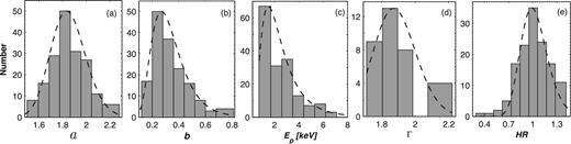
Distribution of the values of various spectral parameters derived from the XRT observations of 1ES 1959+650 in 2016 January–August: photon index at 1 keV, curvature parameter, position of the SED peak, photon index throughout the 0.3–10 keV energy range and HR (with dashed lines representing lognormal fits to the distributions).
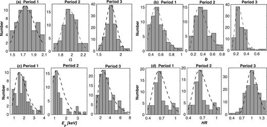
Distribution of the values of spectral parameters in different periods.
Distribution of spectral parameters in different periods: minimum and maximum values (columns 2 and 3, respectively), distribution peak (column 4) and variance (last column).
| Quantity | Min. value | Max. value | Peak value | σ2 |
|---|---|---|---|---|
| (1) | (2) | (3) | (4) | (5) |
| 2016 January–August | ||||
| a | 1.50 | 2.28 | 1.84 | 0.022 |
| b | 0.12 | 0.81 | 0.24 | 0.022 |
| Ep | 0.39 | 12.80 | 1.49 | 2.945 |
| HR | 0.340 | 1.416 | 0.86 | 0.056 |
| Γ | 1.71 | 2.22 | 1.87 | 0.017 |
| Period 1 | ||||
| a | 1.45 | 2.09 | 1.74 | 0.028 |
| b | 0.28 | 0.98 | 0.49 | 0.021 |
| Ep | 0.79 | 3.81 | 1.52 | 0.465 |
| HR | 0.481 | 1.496 | 0.845 | 0.043 |
| Period 2 | ||||
| a | 1.70 | 2.28 | 1.95 | 0.014 |
| b | 0.12 | 0.81 | 0.32 | 0.022 |
| Ep | 0.39 | 3.70 | 1.17 | 0.454 |
| HR | 0.396 | 1.064 | 0.630 | 0.025 |
| Period 3 | ||||
| a | 1.50 | 2.29 | 1.77 | 0.015 |
| b | 0.12 | 0.77 | 0.24 | 0.009 |
| Ep | 0.74 | 12.80 | 2.30 | 3.14 |
| HR | 0.340 | 1.416 | 1.00 | 0.037 |
3.2.1 Photon Index
During 2016 January–August, the source mostly showed hard spectra: the photon index at 1 keV ranged by Δa = 0.78 with the hardest value a = 1.50 ± 0.06 derived from the first 240 s segment of ObsID 00035025254 (June 30, MJD 57569.8; see the corresponding spectrum in Fig. 8, top panel), and 82 per cent of the curved spectra were harder than a = 2 (see Fig. 6a). In the case of 26 spectra, the photon index showed values a < 1.70, and all of them belong to Period 3. In this period, 96.6 per cent of the curved spectra were harder than a = 2.00 and showed the distribution peak at amax = 1.77 (Fig. 7a, third panel) that is uncommon for BLLs (see the spectral results provided by Massaro et al. 2008, Kapanadze et al. 2014, 2016b,c for a comparison) and a similar distribution was shown only by Mrk 501 during 2014 March–October (Kapanadze et al. 2017). Note that a similar situation was seen in Period 1 with practically the same distribution peak (see Table 6 and Fig. 6a, first panel) and four spectra even harder than a = 1.50. Period 2 was characterized by relatively soft spectra: 38.5 per cent showed the values a > 2 and the distribution peaked at a = 1.95 (Fig. 6a, second panel).
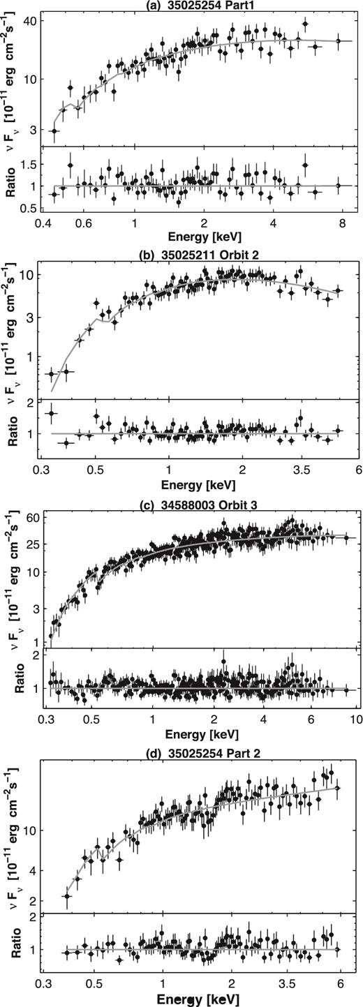
(a)–(c): The three 0.3–10 keV spectra, fitting well with the LP model and yielding the extreme values of the photon index at 1 keV (top spectrum, a = 1.50 ± 0.06), curvature parameter (second panel, b = 0.81 ± 0.12) and the position of the synchrotron SED peak (third panel, Ep = 12.80 ± 0.75 keV). The bottom panel presents the hardest spectrum, fitted well with a simple power law (Γ = 1.71 ± 0.03 and |$\chi ^2_{\rm r}$| = 0.919 with 89 d.o.f.). In each spectrum, the solid line is the best-fitting model, and the bottom panel is the ratio between the observation and the model.
In the whole 2016 January–August period, the source mostly followed a ‘harder-when-brighter’ trend: the spectra with a < 1.7 generally correspond to the unabsorbed 0.3–10 keV flux values larger than |$\overline{F}_{\rm 0.3 \hbox{--} 10\, keV}$| = (4.64 ± 0.01) × 10−10 erg cm−2s−1 which is the weighted mean unabsorbed flux value in this period, while all the spectra softer than a = 2 are characterized by fluxes below this threshold, and the softest spectrum with a = 2.28 ± 0.02 corresponds to F0.3–10 keV = (1.16 ± 0.04) × 10−10 erg cm−2s−1 which is the smallest flux value in the presented period. A ‘harder-when-brighter’ spectral evolution of the source is reflected in Fig. 9(a), where we observe an anticorrelation between the parameter a and 0.3–10 keV flux (see Table 7 for the corresponding Pearson coefficient r and p chance). Note that this trend was observed in all periods (see Table 7 and Fig. 10(a)) which is also evident from Fig. 11(b), exhibiting a time variability of the parameter a along with the unabsorbed 0.3–10 keV flux (Fig. 11a). This plot shows that the photon index varied on different time-scales during 2016 January–August (see also Fig. 12, online material). The largest variability was recorded in Period 2a when the photon index hardened by Δa = 0.60 in 13.8 d, along with an increase by a factor of 3.3 in the unabsorbed 0.3–10 keV flux. A fast strong brightness decay in Period 2b was accompanied by a hardening by Δa = 0.40 in 2.7 d. (Figs 12a and b). The fastest hardening by Δa = 0.16 in 0.5 ks was recorded on July 30 (MJD 57599.7) while the fastest softening by the same value occurred on February 9 (MJD 57427.6). Several other intra-hour hardenings/softenings by Δa = 0.15–0.25 during 0.6–1.5 ks are also revealed which occurred during the IDVs described in Section 3.3 (see Table 4).
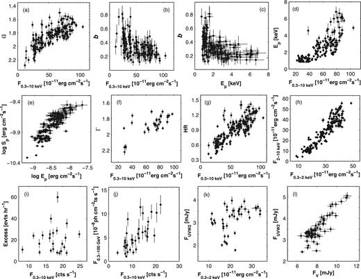
Correlation between the spectral parameters and fluxes in 2016 January–August.
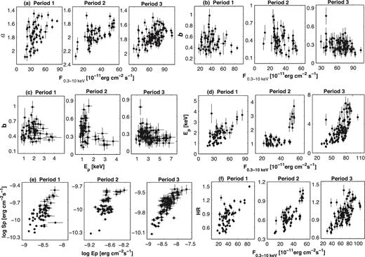
Correlation between the spectral parameters and fluxes in different periods.
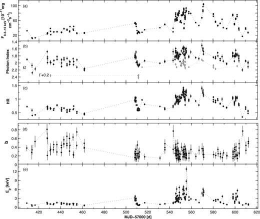
Unabsorbed 0.3–10 keV flux (top panel), photon index (panel b), HR (panel c), curvature parameter (panel d) and Ep (bottom panel) in 2016 January–August as a function of time.
Correlations between the spectral parameters and multiband fluxes (denoted by ‘Fi’ for the particular i band) in the period 2016 January–August and different periods.
| Quantities | r | p |
|---|---|---|
| a and F0.3–10 keV | −0.68(0.05) | 3.22 × 10⁻¹¹ |
| b and F0.3–10 keV | −0.43(0.11) | 6.02 × 10⁻⁶ |
| b and Ep | −0.36(0.13) | 8.74 × 10⁻⁵ |
| Ep and F0.3–10 keV | 0.68(0.08) | 6.31 × 10⁻¹⁰ |
| log Ep and log Sp | 0.74(0.08) | 8.45 × 10⁻¹³ |
| Γ and F0.3–10 keV | −0.66(0.06) | 3.22 × 10⁻¹² |
| HR and F0.3–10 keV | 0.82(0.04) | 1.29 × 10⁻¹⁴ |
| F0.3–2 keV and F2–10 keV | 0.88(0.03) | <10−15 |
| F0.3–10 keV and F0.3–100 GeV | 0.67(0.08) | 1.60 × 10⁻⁷ |
| FUVW2 and FUVM2 | 0.92(0.02) | <10−15 |
| FUVW2 and FUVMW1 | 0.92(0.02) | <10−15 |
| FUVW2 and FUVMW1 | 0.91(0.02) | <10−15 |
| FUVW2 and FU | 0.90(0.03) | <10−15 |
| FUVW2 and FB | 0.89(0.03) | <10−15 |
| FUVW2 and FV | 0.83(0.04) | <10−15 |
| FUVM2 and FUVMW1 | 0.91(0.02) | <10−15 |
| FUVM2 and FU | 0.90(0.03) | <10−15 |
| FUVM2 and FB | 0.89(0.03) | <10−15 |
| FUVM2 and FV | 0.86(0.03) | <10−15 |
| FUVW1 and FU | 0.93(0.02) | <10−15 |
| FUVW1 and FB | 0.92(0.02) | <10−15 |
| FUVW1 and FV | 0.88(0.03) | <10−15 |
| FU and FB | 0.94(0.02) | <10−15 |
| FU and FV | 0.90(0.03) | <10−15 |
| FB and FV | 0.91(0.02) | <10−15 |
| Period 1 | ||
| a and F0.3–10 keV | −0.40(0.11) | 1.35 × 10⁻⁴ |
| HR and F0.3–10 keV | 0.55(0.08) | 2.60 × 10⁻⁶ |
| Ep and F0.3–10 keV | 0.55(0.11) | 7.51 × 10⁻⁶ |
| log Ep and log Sp | 0.53(0.12) | 1.51 × 10⁻⁶ |
| F0.3–2 keV and F2–10 keV | 0.74(0.05) | 7.14 × 10⁻¹³ |
| F0.3–10 keV and F0.3–100 GeV | 0.47(0.12) | 1.21 × 10⁻⁴ |
| Period 2 | ||
| a and F0.3–10 keV | −0.51(0.11) | 7.04 × 10⁻⁶ |
| b and F0.3–10 keV | −0.31(0.12) | 2.96 × 10⁻³ |
| HR and F0.3–10 keV | 0.67(0.07) | 6.02 × 10⁻¹¹ |
| Ep and F0.3–10 keV | 0.48(0.12) | 1.33 × 10⁻⁵ |
| log Ep and log Sp | 0.51(0.12) | 9.62 × 10⁻⁵ |
| b and Ep | −0.34(0.14) | 2.55 × 10⁻⁴ |
| F0.3–2 keV and F2–10 keV | 0.81(0.04) | 1.19 × 10⁻¹³ |
| Period 3 | ||
| a and F0.3–10 keV | −0.44(0.10) | 5.80 × 10⁻⁶ |
| b and F0.3–10 keV | −0.26(0.12) | 6.69 × 10⁻³ |
| HR and F0.3–10 keV | 0.59(0.08) | 9.80 × 10⁻¹¹ |
| Ep and F0.3–10 keV | 0.62(0.08) | 5.54 × 10⁻⁹ |
| b and Ep | −0.32(0.11) | 7.44 × 10⁻⁴ |
| log Ep and log Sp | 0.69(0.08) | 3.14 × 10⁻¹² |
| F0.3–2 keV and F2–10 keV | 0.83(0.03) | 1.19 × 10⁻¹³ |
3.2.2 Spectral curvature
Although the curvature parameter also showed a wide range12 between b = 0.11 ± 0.07 and b = 0.81 ± 0.12 (see the middle panel of Fig. 8 for the spectrum with the largest curvature), its values were mainly relatively small with b < 0.35, and only 5.7 per cent of the curved spectra showed b > 0.50 (Fig. 6b). They were mostly included in the interval b = 0.20–0.40 (75 per cent). Note that Period 2 was characterized by relatively strongly curved spectra compared to Period 3: the distribution peak is shifted by Δbpeak = 0.08 towards larger values, and 69 per cent of the spectra with b > 0.4 belong to this period (see Table 6 and Fig. 7b). Note that the mean value of the curvature parameter was the largest in Period 2a (|$\bar{b}$| = 0.45 ± 0.01) while it was significantly smaller in Period 2b (|$\bar{b}$| = 0.25 ± 0.02). The sub-periods of Period 3 were also characterized by small mean values of the curvature parameter, ranging between |$\bar{b}$| = 0.23 ± 0.02 (Period 3b) and |$\bar{b}$| = 0.28 ± 0.02 (Period 3b). Note that the source showed significantly stronger curved spectra in Period 1 than in Periods 2 and 3 and during 2005–2014 (Paper I; Kapanadze et al. 2016b): from the broad range b = 0.28–0.98, 73 per cent of the values were larger than b = 0.40, and the distribution maximum was shifted by 0.17–0.25 towards higher values compared to Periods 2 and 3 (see the corresponding discussion in Section 4.3).
The values of the parameter b from the whole period 2016 January–August showed a weak anticorrelation with the unabsorbed 0.3–10 keV flux (see Fig. 9b and Table 7), and we observe this trend also in particular Periods 2 and 3 (Fig. 10b and Table 7, although the correlation is very weak in the last period). However, no significant correlation between these quantities was revealed for Period 1 (r = −0.08, p = 0.55; Fig. 10b). Moreover, the parameter b showed a weak anticorrelation with Ep in 2016 January–August (Fig. 9c), and this trend was also observed in Periods 2 and 3 separately (see Fig. 10c and Table 3). No significant b–Ep correlation occurred in Period 1 (Fig. 10c).
In all periods, the parameter b varied on diverse time-scales (Figs 11d and 12). The largest intra-hour variability was recorded during the second orbit of ObsID 00035025211 (February 9) lasting less than 1.2 ks. While its first and third segments showed b = 0.60(0.13)–0.61(0.11), the second orbit showed a significantly smaller curvature (b = 0.21 ± 0.11; a PL fit was rejected by the aforementioned tests). A similar variability was recorded in the case of ObsID 00035025220 (MJD 57543.3) when the curvature parameter increased by Δb = 0.42 in about 1 ks. In Period 1, the fastest variability in the spectral curvature was a decrease by Δb = 0.31 in 1.26 h. Note that these events are related to the IDVs presented in the previous sections (see Table 4).
3.2.3 The position of the SED peak
The parameter Ep, calculated via equation (3), showed an extremely large range from 0.39 ± 0.12 keV to 12.80 ± 0.86 keV in 2016 January–August (see Fig. 8c for the spectrum corresponding to the largest value of this parameter). However, the values Ep ≲0.80 keV and Ep ≳8 keV (derived from the X-ray spectral analysis), the intrinsic position of the synchrotron SED peak is poorly constrained by the XRT observation, and these Ep values should be considered as upper limits to the intrinsic ones (see Kapanadze et al. 2014, 2016b). We have not used them for the construction of the histograms presented in Figs 6(c) and 7(c), or when searching for the correlations of Ep with other spectral parameters (or fluxes). Note that Ep < 0.80 keV was the case only for the 7.1 per cent of the curved spectra, and the vast majority (11 out of 13) belong to Period 2. As for the values above 0.80 keV, 53 per cent are larger than Ep = 2 keV (the dividing line between the soft and hard X-rays). Note that the vast majority of hard X-ray peaking spectra belong to Period 3, while only nine spectra (10.3 per cent) from Period 1 show Ep > 2 keV, and this result is reflected in the corresponding histograms which show the distribution peak in the hard X-ray band for Period 3, in contrast to the previous period (see Fig. 7c and Table 6). Among different sub-periods, the weighted mean values of this parameter ranged between |$\bar{E_{\rm p}}$| = 1.04 ± 0.04 keV (Period 1b) and |$\bar{E_{\rm p}}$| = 3.68 ± 0.10 keV (Period 3b).
This parameter showed a positive correlation with the 0.3–10 keV flux as in the whole 2016 January–August period, as in particular Periods 1–3 (Fig. 9d). The correlated Ep–F0.3–10 keV variability is also evident from Figs 11(e) and 12(a)–(f) (online material), where Ep is plotted versus time. We see that the peaks in the unabsorbed 0.3–10 keV flux and the position of the SED peak mostly coincided with each other. For example, the maximum value of the Ep is derived from the spectrum extracted from the third orbit of ObsID 00034588003 which also shows the maximum 0.3–10 keV flux in Period 3b (Fig. 12d). During the X-ray flares described in Section 3.2, the position of the SED peak shifted by 1.20–10.30 keV towards higher energies with increasing flux, and moved back to lower energies as source became progressively fainter. The most dramatic variability was observed during June 15–16 when Ep shifted from 2.49 ± 0.26 keV to the aforementioned maximum value in 1.13 d, and then declined by 8.8 keV in 2.4 d. Although the whole data set from Period 2 shows a positive Ep–F0.3–10 keV correlation, the SED peak position mainly did not follow the flux variability during Period 2a (see Fig. 12a, online material), and made an exclusion from the general trend in Fig. 10(d) (second panel). Moreover, there was another exception from the correlated variability: the parameter Ep showed a fast increase by 4.2 keV in 0.4 d on MJD 57546.5 when the source did not show significant changes in the flux (Fig. 12c, online material). On the sub-hour time-scales, Ep showed increases by 0.41–2.20 keV and declines by 1.19–1.83 keV during 0.50–1.45 ks and 0.50–0.80 ks, respectively. Generally, these very fast variations were related to the fast IDVs presented in Section 3.3 (see also Table 4).
A correlated variability of Ep and F0.3–10 keV also occurred in Period 1 (see Figs 10d and 12h, Paper I), although the range and the maximum value of the synchrotron SED peak location (about 3 keV and 3.81 ± 1.02 keV, respectively) were significantly smaller than in Period 3.
3.2.4 Power-law spectra
Out of 197 spectra, 34 do not show a significant curvature, and their fit with the LP model did not yield a better statistic than a single PL model. Therefore, we chose the latter model for these spectra (see Table 8 for the results). Note that the broad-band SEDs constructed for these observations show the presence of the synchrotron SED peak in the aforementioned range of the parameter Ep. Therefore, a better statistic for the PL fit compared to the LP one cannot be related to the presence of the synchrotron SED peak far from the instrumental range of the XRT when it is difficult to evaluate a possible curvature, and a simple PL model gives relatively better description of the spectrum (see Massaro et al. 2008). These spectra are mainly hard (similar to the LP spectra): 88 per cent show Γ < 2, and all the remaining four spectra with Γ = 2.15(0.03)–2.22(0.04) belong to Period 2a (see Fig. 6d for the distribution of the photon index, and Fig. 8d for the hardest PL spectrum). The mean weighted value of Γ in Period 3 ranged from 1.82 ± 0.01 (Period 3a) to 1.89 ± 0.03 (Period 3d).
The results of the XRT spectral analysis with a simple PL model (extract). Unabsorbed 0.3–2 keV, 2–10 keV and 0.3–10 keV fluxes (columns 5–7) are given in erg cm−2 s−1.
| ObsId | Γ | K | χ2 (d.o.f.) | logF0.3–2 keV | logF2–10 keV | logF0.3–10 keV | HR |
|---|---|---|---|---|---|---|---|
| (1) | (2) | (3) | (4) | (5) | (6) | (7) | (8) |
| 00035025213 Orbit 2 | 2.16(0.04) | 5.93(0.15) | 0.943/94 | −9.725(0.014) | −9.918(0.021) | −9.501(0.009) | 0.641(0.033) |
| 00034532008 Part 1 (500 s) | 2.16(0.03) | 5.54(0.11) | 1.040/131 | −9.754(0.011) | −9.949(0.017) | −9.539(0.008) | 0.638(0.030) |
| 34532009 Part 2 (400 s) | 2.15(0.03) | 5.84(0.13) | 0.953/79 | −9.733(0.012) | −9.918(0.020) | −9.515(0.009) | 0.653(0.035) |
| Part 3 (340 s) | 2.22(0.04) | 5.73(0.14) | 1.072/90 | −9.731(0.014) | −9.970(0.022) | −9.536(0.010) | 0.577(0.035) |
Note that some XRT observations of 1ES 1959+650 in Periods 2 and 3 showed the presence of both LP and PL spectra extracted from its different segments or orbits. An example is presented in Fig. 8, where the first 240 s segment of ObsID 00035025254 (July 2, the observation with the highest historical 0.3–10 keV flux) shows a curved spectrum, while the curvature is absent in the spectrum extracted from the second 240 s segment which is well fit by the PL model (bottom panel). We found only one PL spectrum in Period 1 (see Paper I), in contrast to the 2016 January–August period.
The PL spectra are found in diverse brightness states of the source, and followed a ‘harder-when-brighter’ trend similar to the LP spectra (see Figs 9f, 11b and 12b–e, online material). The photon index Γ varied on diverse time-scales, similar to the parameter a.
3.2.5 Hardness ratio and spectral hysteresis
The values of the HR, derived from LP and PL spectra, showed a wide range ΔHR = 1.076 in 2016 January–August, and 38 per cent are larger than HR = 1 (see Tables 5, 8 and Fig. 6e) that is also uncommon for BLLs (see the spectral results provided by Kapanadze et al. 2014, 2016b,c for a comparison). However, Mrk 501 showed a harder distribution of this parameter with 76.6 per cent of the spectra characterized by HR ≥1 in 2014 March–October (Kapanadze et al. 2017).
The largest HR is derived from the PL spectrum whose X-ray SED is shown in Fig. 8(d) and the corresponding 0.3–10 keV flux is one of the largest in the period studied here. The histograms corresponding to Period 2 and exhibit the distribution peaks at about HR = 0.65 and HR = 1.00 (Fig. 6e), respectively. This result confirms that the 0.3–10 keV spectra of 1ES 1959+650 were generally significantly harder in Period 3 than those in the previous period (as discussed in Section 3.2.1). Note that only three spectra out of 75 with HR >1 belong to Period 2, while the vast majority of these spectra belong to the next period. The behaviour of the HR also confirms the dominance of the aforementioned ‘harder-when-brighter’ spectral evolution of our target during X-ray flares in all periods (see Fig 9g and Table 7).
As for Period 1, it also showed a wide range of values with ΔHR = 1.015 and HRmax = 1.496 ± 0.031 which slightly exceeds the largest HR in Period 3 (see Fig. 7d and Table 6). However, the latter showed the distribution peak at significantly larger value.
The parameter HR also showed a variability on diverse time-scales (Figs 11c and 12a–g). On the intra-hour ones, it exhibited several increases by 16–22 per cent in 0.42–1.52 ks and declines by 19–28 per cent in 0.60–1.02 ks (generally related to the 0.3–10 keV IDVs; see Table 4).
We performed a search of the spectral hysteresis, i.e. a loop track of a blazars state in a hardness–intensity diagram (Böttcher & Dermer 2010). For this purpose, we constructed a HR–0.3–10 keV flux plane (see Section 4.5 for its physical implication) for each period (Fig. 13). First, we constructed it for Period 3 (when the source showed strongest X-ray flares), splitting this plane into several parts for a better resolution. In the HR–flux plane, the source exhibited a complex behaviour, and its spectral evolution followed a clockwise (CW) or a counterclockwise (CCW) loops during the short-term X-ray flares presented in Section 3.1.3, or showed a change from a CW loop into the opposite one and vice versa within a single flare.
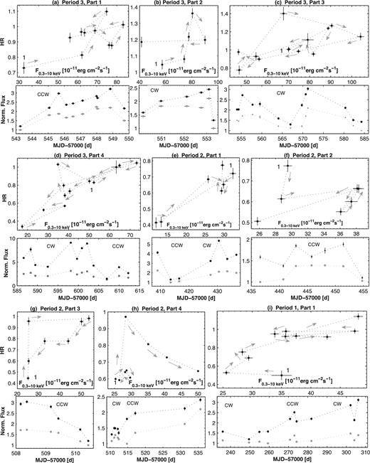
Spectral hysteresis in different epochs, along with the normalized soft 0.3–2 keV (grey points) and hard 2–10 keV (black points) fluxes plotted versus time (extract). The light curves for hard fluxes are shifted arbitrarily for a better resolution. In each plane, the start point is denoted by ‘1’. Grey arrows show the direction of increasing time. See the next page for Figs 13(j)–(l).
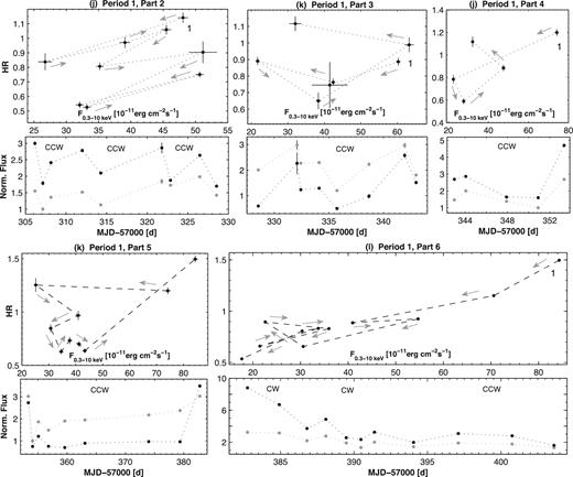
– continued
In Period 3, 1ES 1959+650 followed a CCW-type trend during MJD 57543–57550 (Fig. 13a; the flare in Period 3a) and MJD 57605–612 (Fig. 13d; a minor flare at the and of Period 3), while most of this period (MJD 550–605) was dominated by clockwise loops: the last low-amplitude flare with a fast decline in Period 3a (Fig. 13b); the flares in Periods 3b and 3c (Fig. 13c); a minor flare at the end of Period 3c and a double-peak flare in Period 3d (Fig. 13d). Figs 13(b) and (c) show some evidence of a soft lag (e.g. a soft X-ray flare was started with a possible delay at MJD∼57552 and 56770, or a delayed peak in the soft X-ray light curve at MJD∼57556), as expected from a CW-type spectral evolution (Takahashi et al. 1996). However, we cannot use the local cross-correlation function (Max-Moerbeck et al. 2014) technique to draw a firm conclusion and derive exact values of the hard lag, since the duration of each observation during this flare is much shorter than the time intervals between them.
In contrast, the majority of Period 2 was dominated by a CCW-type spectral evolution (MJD 57410–57455, 508–510, 514–535; see Figs 13e–h), and a similar situation was also found during the flares observed in period 1 (MJD 56270-56281, 56305–56382, 56394–56403; Figs 13 i–l).
Our spectral study shows that the majority of the 0.3–10 keV spectra of 1ES 1959+650, obtained with the XRT observations during 2016 June–August, were curved and described by the log-parabola model well with broad ranges of photon index, HR and synchrotron SED peak location. High brightness states and strong fast intra-day variability of the 0.3–2 keV and 2–10 keV fluxes, which was stronger towards higher frequencies, allowed us to detect very fast spectral variability. Namely, a hardening by Δa = 0.16 in 0.5 ks, an increase of the curvature parameter by 0.42 in 1 ks and a shift of the synchrotron SED peak position by 2.2 keV towards higher energies in 1.45 h are the fastest spectral variability events reported for this source to date (found by us in this study). The spectral parameters varied on diverse time-scales, and the source exhibited a ‘harder-when-brighter’ spectral evolution with the flux variability.
4 DISCUSSION
In this section, we discuss the results from the MWL flux variability and X-ray spectral study of 1ES 1959+650 along with those published to date.
4.1 Flux variability
4.1.1 Variability character
During 1 yr, 1ES 1959+650 showed strong and prolonged X-ray flaring activity in 2015 August–2016 January and 2016 June–August, as revealed by the densely sampled XRT observations. On average, the source showed significantly higher brightness state during the second flare with a weighted mean 0.3–10 keV count rate of 15.25 versus 9.72 cts s−1 from the first one. However, the latter is 65 per cent higher than that derived from the previous 10.35 yr period of the Swift observations of our target (see Fig. 2). In period 1, 1ES 1959+650 became the third BLL source (after Mrk 421 and Mrk 501) with a 0.3–10 keV count rate exceeding the threshold of 20 cts s−1. Moreover, the source exceeded this threshold seven times in Period 3 (versus 2 occasions in Period 1), and a new highest historical rate was recorded which is 8 per cent larger than the previous one from Period 1. The 33 per cent of XRT observations in Period 3 yielded the rates larger than 15 cts s−1 which occurred only three times in Period 1. Both periods were characterized by strong shorter term flares by a factor of 1.9–4.7 with very short flux increase or decay phases lasting 0.2–3.4 d.
Note that Period 3 is also remarkable for another fact: the source showed an unabsorbed 0.3–10 keV flux larger than 10−9 erg cm−2 s−1 for the first time since the start of Swift observations [see Fig. 11a; the maximum 0.3–10 keV flux in Period 1 was (8.43 ± 0.10)× 10−10 erg cm−2 s−1]. As for the 2–10 keV flux, it reached a value of (5.56 ± 0.17)× 10−10 erg cm−2 s−1 (10 per cent larger compared to that in Period 1). From the past X-ray campaigns of 1ES 1959+650, the largest 2–10 keV flux of 2.93 × 10⁻¹⁰ erg cm−2 s−1 was reported by Perlman et al. (2005) from the XMM–Newton pointing performed in 2002 November, while the lowest value of 8.40 × 10⁻¹² erg cm−2 s−1 was found by Giebels et al. (2002) from the PCA observation of 2000 September 2. Using the latter value, we obtain that the 2–10 keV flux varied by a factor of 66 in 2000–2016.
Along with the higher X-ray states, Period 3 was also characterized by a strong TeV-band activity. The source was detected with the FACT telescope only 5 times in Period 1 above the 3σ significance with no evident variability, while it was detected 35 times and showed three strong TeV flares by a factor of 5.6–9.5 in Period 3 (Fig. 2b). Although the weighted mean 0.3–100 GeV flux was also higher (5.27 ± 0.30 versus 4.84 ± 0.13, in units of 10−8 photons cm−2 s−1) and showed more detections above the threshold 10−7 photons cm−2 s−1 in the latter period, the LAT-band flux was more variable and exhibited a larger maximum value in Period 1 (see Fig. 2c). A similar situation was seen in the UVOT bands: the source exhibited larger maximum and mean weighted values in Period 3, while it was more variable in Period 1 (especially, in the bands U–UVW2; see Figs 2d and e).
The strong flares were separated by a period lasting ∼5.5 months during which the source showed relatively modest X-ray brightness states with the maximum and weighted mean count rates of 13.54 cts s−1 (comparable to the maximum historical rate before 2015 August) and 7.74 cts s−1, respectively, and underwent shorter term flares by a factor of 2.1–3.6 which exhibited significantly slower brightness increase than those observed in Periods 1 and 3. Similar to Period 1, the source was detected only a few times by FACT above the 3σ significance and did not show a significant variability also in this period. Maximum-to-minimum flux ratios in the LAT-band were also comparable in both these periods, but the 0.3–100 GeV flux did not exceed the value of 6.2 × 10⁻⁸ photons cm−2 s−1, and its weighted mean value was smaller by a factor of 2 in Period 2. In this period, the UVOT fluxes showed smaller maximum/mean values and variability than in Period 3, although the source was on average brighter at the UV–optical frequencies than in Period 1.
4.1.2 Intra-day variability
During 2016 January–August, our target was also active on intra-day time-scales, and the corresponding duty cycle (DC, the fraction of the total observation time during which the the source was variable; Romero et al. 1999) of the 0.3–10 keV IDVs is 52.5 per cent. Note that the source showed fewer IDVs in Period 1 (DC = 28.1 per cent, including those detected with the 99.5 per cent confidence level), although the later was characterized by the largest IDV when the 0.3–10 keV count rate dropped by a factor of 2.3 in about 18 h on 2015 November 27–28, and four IDVs with the 99.5 per cent confidence level occurred within 0.48–0.84 ks. Note that a brightness drop by the same factor in a slightly smaller interval (17.2 h) was also observed in Period 3 which was also notable for several very fast IDVs with the 99.9 per cent confidence level in 0.24–0.75 ks. Moreover, many IDVs in 2016 January–August are revealed via the combination of the 2–3 XRT observations performed within a day that occurred less frequently in Period 1. Note that our target was significantly less variable on intra-day time-scales than Mrk 421 in 2013 January–May: the duty cycle of X-ray IDVs amounted to 83 and 99 per cent for the XRT and NuSTAR observations of this source, respectively (Kapanadze et al. 2016c).
It is important to check an occurrence of IDVs in diverse brightness states that can provide us with a hint at the possible unstable mechanisms. Namely, the 0.3–10 keV IDVs observed during flaring epochs were in favour of the shock-in-jet scenario (interaction between the propagating shock front and the jet inhomogeneities; Sokolov, Marscher & McHardy 2004, while those triggered by other unstable mechanisms occurring in the innermost blazar area should be more easily detectable in the target's low states, i. e. the variable emission, produced in the vicinity of the central supermassive black hole will not be ‘shadowed’ by the huge amount of the flux generated by the emission zone following the shock front (see e.g. Mangalam & Wiita 1993; Kapanadze et al. 2014). Similar to the behaviour seen in 2005–2014, X-ray IDVs in 1ES 1959+650 were mainly detected during higher brightness states in Period 3 while the situation is opposite in Period 1 (see the area right to vertical dashed lines in Figs 14a–c). In Periods 1–3, we do not observe an anticorrelation between the corresponding fractional amplitudes and unabsorbed 0.3–10 keV flux (in contrast to that in 2005–2014; see Kapanadze et al. 2016b) and the IDVs with the largest Fvar were observed during higher brightness states in each period.
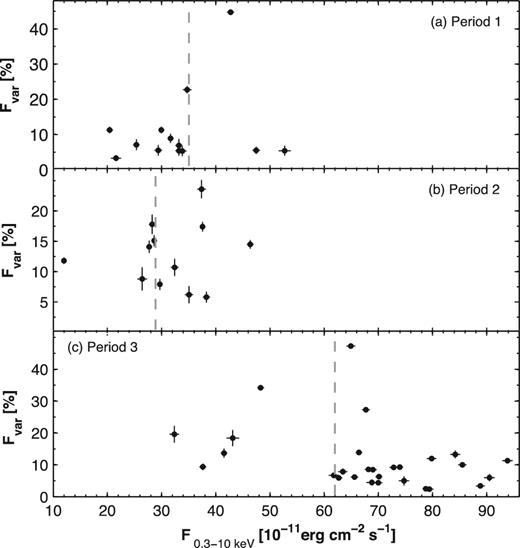
Fractional variability amplitude of the X-ray IDVs detected with the 99.9 per cent confidence level as a function of the XRT flux in different periods. A vertical dashed line in each plot stands for the weighted mean 0.3–10 keV flux in the given period.
4.1.3 Fractional variability amplitude
In the Fvar–logν plane, where the Fvar values from each band are calculated using all the available data obtained with various instruments during 2005–2016, 1ES 1959+65 shows a double-peaked shape with the highest variability in the X-ray and VHE bands (Fig. 15a). Note that the value of Fvar is known to be dependent on the data sampling, and this result should be interpreted with a caution. Generally, Fvar was derived using the individual single-day measurements of our target, except for MAXI, BAT and LAT, for which, because of the limited sensitivity, we used data integrated over 1–4 weeks, and for the calculation of fractional variability amplitude from the MAXI, BAT and LAT observations, we used only the flux values from those time bins when the source was detected with the significances described in Section 2. A similar shape is evident from Fig. 15(d), where a log ν–Fvar plot is constructed separately for Period 3 and the 3-d binned LAT fluxes are used to derive the fractional variability amplitude. The same was done for Periods 1 and 2 (Figs 15 b–c), although no FACT and MAXI data points were available for these cases and, in addition, no BAT point was available for Period 2. Therefore, we cannot draw a firm conclusion about the presence of a double-peaked fractional variability in these periods. This shape, exhibiting the highest variability in the X-ray and VHE bands, was interpreted as resulting from a correlation between the synchrotron and IC peaks by Furniss et al. (2015), and as an indication that the electron energy distribution is most variable at highest energies (in the framework of one-zone SSC scenarios; see Aleksic et al. 2015b). Although a limited sensitivity and the use of larger time bins can underestimate Fvar values for some instruments, a double-peak shape in the Fvar–logν plane seems to be inherent for HBLs, and it has been reported by various authors for Mrk 421 from the MWL campaign performed in various epochs (Aleksic et al. 2015b; Balokovic et al. 2016; Kapanadze et al. 2016c), Mrk 501 in 2014 March–October (Kapanadze et al. 2017).
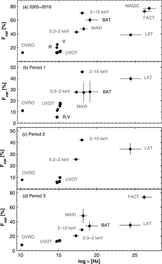
Fractional rms variability amplitude as a function of the energy in different periods.
4.2 Interband cross-correlations
4.2.1 Soft–hard X-rays and X-ray–TeV correlation
The unabsorbed soft 0.3–2 keV flux showed a strong positive correlation with the hard 2–10 keV flux in all periods (see Table 7 and Fig. 9h). In each sub-period, the corresponding light curves mostly followed each other closely. However, the hard flux varied by a larger amplitude than the soft one in each period or sub-period (see Table 3 and Fig. 13), yielding a strong spectral variability. This difference was the largest in Period 3d when the 0.3–2 keV flux varied by a factor of 2.92, while we observe a variability by a factor of 8.73 in the 2–10 keV band. Note that the maximum hard X-ray flux for the whole 2016 January–August period was 12 per cent larger than the soft one, and the hard flux generally exceeded the soft one during Periods 3a–3d. A similar situation was seen in Period 1 (with even larger difference between the hard and soft fluxes), and this result is also uncommon for BLLs. Similar results were reported for Mrk 421 (during the extreme X-ray outbursts in 2013 April; Kapanadze et al. 2016c) and Mrk 501 (during the 2014 flare; Kapanadze et al. 2017). However, Period 2 was an exception in this regard (especially Period1a, when the maximum soft flux was 44 per cent larger than the maximum 2–10 keV one).
In Period 3, when the source were detected by FACT frequently, there was a lack of a correlated X-ray–TeV variability. While the VHE peaks on MJD 57545, 57552, 57570 are observed in the epoch of increasing X-ray activity (Figs 3c and e), a strong TeV flare by a factor of 9.4 occurred around MJD 57581 when the source showed a decreasing X-ray brightness (Fig. 3e).13 Furthermore, the source exhibited a low TeV state in the epochs of the second X-ray peak in Period 2b (see Fig. 3b), enhanced X-ray–HE activity around MJD 57548 (Fig. 3c), X-ray flares in Periods 3b14 and 3d (see Figs 3d and f, respectively). Consequently, the simultaneous X-ray and TeV data do not show a significant correlation (Fig. 9i).15
Note that a lack of the X-ray–TeV correlation is familiar to 1ES 1959+650. The source became prominent with its ‘orphan’ TeV flare on 2002 June 4 (Krawczynski et al. 2004), and a similar situation occurred in 2009 May and 2012 May (Kapanadze et al. 2016b). A strong X-ray variability was not accompanied by a flaring behaviour in the VHE band during the 2003 MWL observations (Gutierrez et al. 2006). The source showed a similar behaviour in 2006 May, 2007 November, 2010 May–June and September (Tagliaferri et al. 2008; Kapanadze et al. 2016b).
4.2.2 X-rays versus HE and optical–UV emissions
The source showed a positive correlation between the 0.3–10 keV and 0.3–100 Gev fluxes in Period 1 and Periods 2 and 3,16 and it was stronger in the second case (see Fig. 9 j and Table 7). In contrast, this correlation was absent in Mrk 421 (during 2013 January–June; Kapanadze et al. 2016c) and Mrk 501 (in 2014 March–August; Kapanadze et al. 2017). However, these sources exhibited positive correlations between the LAT and UVOT-band fluxes. Note that Tramacere et al. (2009) suggested the possibility of a positive correlation between the UV and MeV/GeV-band fluxes due to the effect of the Klein–Nishina (K–N) suppression in the IC process, leading to the UV photons being upscattered most efficiently at the GeV energies by the electrons radiating in X-rays, and this suggestion is in agreement with the aforementioned correlation between the UVOT and LAT-band fluxes and uncorrelated variability of the XRT and HE fluxes in Mrk 421 and Mrk 501. In contrast to these HBLs, the positive correlation of the 0.3–100 GeV flux with the X-ray flux and absence of significant correlation with the UVOT-band fluxes in 1ES 1959+650 allows us to suggest that the upscatter of X-ray photons to the MeV–GeV energies in the K–N regime possibly was more efficient during the flares in the 2015 August – 2016 August period than the upscatter of UV photons to these energies in the Thomson regime. However, the obtained positive F0.3–10keV–F0.3–100GeV correlation is based on the 3-d binned data in both bands. Due to faintness of our target in the LAT-band (related to the shape of its broad-band SED), we cannot obtain credible values of the 0.3–100 GeV fluxes on the time-scales shorter than 3 d for most of the LAT observations of 1ES 1959+650 performed in the period 2015 August–2016 August and check the presence of the aforementioned correlation on these time-scales (in contrast to Mrk 421 in the first half of 2013 when the source showed an absence of the F0.3–10keV–F0.3–100GeV correlation between the daily binned XRT-band and LAT-band fluxes; see Kapanadze et al. 2016c). Nevertheless, the source showed a strong X-ray variability on time-scales t <3 d, sometimes even on the intra-day ones (see Sections 3.1.3–3.1.4, 4.1 and Paper I) which is less expected in the 0.3–100 GeV energy range (see the discussion in Section 4.1.3). Moreover, some 3-d intervals from the period 2016 January–August, corresponding to the target's detection below the 3σ significance, are not included in the correlation study. Due to these reasons, we cannot draw firm conclusion about the relevance of the detected F0.3–10keV–F0.3–100GeV correlations and, hence, about the importance of the upscatter of X-ray photons to the MeV–GeV energies in the K–N regime during Periods 1–3.
As we have seen in Section 3.2, the optical–UV band light curves sometimes showed a decline when the source had undergone an X-ray flare. A similar situation was reported by Aleksic et al. (2015a) for Mrk 421 from the MWL campaign in 2009 January–June, and explained it via the hardening in the electron energy distribution that can shift the entire synchrotron bump to higher energies. If the spectral index of the electron population is getting harder, the emission at the rising segment of the synchrotron SED (radio–UV) will decline, while that on the decreasing segment (X-rays) increases. The general trend of shifting the synchrotron SED peak location towards higher energies with the increasing X-ray flux in 1es 1959+650 (see Section 3.2.3) also favours this scenario. Finally, the optical–UV fluxes from the UVOT observations showed a strong correlation to each other in all periods (see Table 7, Figs 1–3 and 9l), and did not exhibit any behaviour hinting that these originate from different electron populations.
4.3 Spectral curvature
The distribution of the values of the curvature parameter can hint at the plausible acceleration mechanism of the X-ray emitting particles since a curved photon spectrum is produced by the electron population with a LP energy spectrum (Massaro, Paggi & Cavaliere 2011). The latter can be established by means of first-order Fermi mechanism at the front of relativistic shock wave when the acceleration probability is a decreasing function of the electron energy (‘energy-dependent acceleration probability process’, EDAP), and a positive correlation between a and b is expected in that case (M04). However, we have not found such a correlation for our target neither in the whole 2016 January–August, nor in individual sub-periods. No positive correlation between the parameters a and b was also evident in Period 1.
Another plausible mechanism for the establishment of a curved energy spectrum is stochastic acceleration of charged particles which can be related to the magnetic turbulence close to a shock front (Tramacere et al. 2009). The study of Massaro et al. (2011) showed that the electrons in the jets of TeV detected HBLs should undergo a more efficient stochastic acceleration than those of the TeV-undetected HBLs, and relatively low values of the curvature parameter (b ⋍ 0.3) are expected in that case. Our spectral study of 1ES 1959+650 shows that the source ‘behaved’ according to this scenario in 2016 January–August, showing relatively small spectral curvature and an anticorrelation between the parameters b and Ep, also expected in the case of the efficient stochastic acceleration (Tramacere et al. 2009). Namely, this anticorrelation was observed in both Periods 2 and 3 (perhaps, weakly, probably due to ‘contamination’, by other types of the acceleration or cooling processes; see K16b), which also showed, on average, significantly lower values of the parameter b with the distribution peaks bpeak = 0.24–0.32 and the values mostly below b = 0.35. Moreover, both periods were also characterized by anticorrelation between the spectral curvature and unabsorbed 0.3–10 keV flux, i.e. the larger values of the parameter b are inherent to the observations performed in relatively low X-ray states, and became smaller (corresponding to the widening of the synchrotron SED) with increasing brightness.
In Paper I, however, we concluded that there was less efficient stochastic acceleration during the strong flaring activity in Period 1 due to the larger spectral curvature than in the previous 2005–2014 period, and absence of anticorrelation between the parameters b and Ep. Note also a large decrease of the mean value of the curvature parameter from |$\bar{b}$| = 0.45 in Period 2a (just following Period 1) to |$\bar{b}$| = 0.25 in Period 2b, separated by more than 3 months from the period of the less efficient stochastic acceleration. This results may hint at the progressively increasing importance of this mechanism in the the jet of our target with time after Period 1.
Along with mostly small spectral curvature, the 2016 January–August period was remarkable for a relatively frequent occurrence of PL spectra (15.7 per cent of all spectra) compared to the previous XRT observations of 1ES 1959+650 (1.6 per cent in 2005–2014 and only one PL spectrum in 2015 August–2016 January; Kapanadze et al. 2016a,b). This result leads to the suggestion that the jet of our target was in a state favouring processes establishing a PL-distribution of X-ray emitting particles with energy in the period presented here more so than in past years. However, the PL spectra were more frequently observed during the strong prolonged X-ray flaring activity of Mrk 501 in 2014 March–October (24 per cent; Kapanadze et al. 2017).
4.4 The position of synchrotron SED peak
Our spectral study of 1ES 1959+650 has revealed a very wide range of the position of the SED peak with Ep = 0.39(0.12)–12.80(0.86) keV during 2016 January–August, and this is the first case when this peak moved beyond 10 keV. In Period 1, the values of the parameter Ep fell in the aforementioned interval and the maximum value was less than 4 keV. Note that this parameter, on average, showed significantly smaller values during the XRT observations in 2005–2014 (0.12–1.84 keV; K16a), and small values were also found from the BeppoSAX observations in 2001 September (0.1–0.7 keV; Tagliaferri et al. 2003). The fact that most spectra from Period 3 showed Ep >2 and the overall range of the peak frequency νp = Ep/h during 2001–2016 logΔνp = 2.11 Hz (that happens rarely in HBLs), imply extreme changes in the physical conditions in these HBLs from epoch to epoch. On the other hand, this result is less extreme than that for Mrk 421 and Mrk 501. The former showed the synchrotron SED peak position ranging from a few eV to 18.5 keV during 2013 February–April (corresponding to logΔνp ≈3.5 Hz). As for Mrk 501, it showed a large shift in the Ep parameter from 0.79 ± 0.08 keV to 21.98 ± 2.81 keV (with 95 per cent of the values larger than 2 keV) during the strong and prolonged X-ray activity in 2014 March–October (Kapanadze et al. 2017), and the SED peak shifted beyond 100 keV during the giant X-ray outburst in 1997 April (Tavecchio et al. 2001). That yields an overall range of the peak frequency logΔνp >2.10 Hz during 1997–2016.
4.5 Spectral hysteresis
The hysteresis patterns in the HR–flux plane incorporate the signatures of the single particle acceleration events (Kirk, Rieger & Mastichiadis 1998) and, hence, they are very important in the study of X-ray flares in blazars. Consequently, these patterns allow us. to draw conclusions about the interplay between electron acceleration (τacc), synchrotron cooling (τsyn) and flux variability (τvar) time-scales. In this plane, the following patterns are expected (Cui 2004): (a) a clockwise (CW) loop, if τsyn ≫ τvar ≫ τacc or τsyn ≫ τacc ≫ τvar. In these cases, the spectrum becomes softer in the source's declining phase and harder in the brightening phase, indicating that the hard X-rays variability leads that in the soft X-rays both during the increase and the decrease of brightness (Takahashi et al. 1996); (b) a counterclockwise (CCW) loop, when the acceleration, synchrotron cooling and flux variability time-scales are nearly equal to each other. In that case, electrons are gradually accelerated and the information about the occurrence of a flare propagates from lower to higher electron energies, and we therefore should observe a hard lag (Ravasio et al. 2004).
Our study of the hysteresis patterns in 1ES 1959+650 shows that the extreme spectral variability during the two extreme long-term X-ray flares, which occurred in our target within 1 yr, exhibited a different interplay between electron acceleration, synchrotron cooling and flux variability time-scales. The second flare mainly showed CW loops in the HR–flux plane, and this is consistent with the dominance of synchrotron cooling, since its time-scale is shorter at higher energies (Falcone et al. 2004). In contrast, the flare in 2015 August–2016 January (and the subsequent 5.5-month period as well) was dominated by CCW loops. As for the Swift-XRT observations of our target during 2005–2014, it exhibited pure or dominantly CW loops in the HR-flux plane (Kapanadze et al. 2016b). The episodic changes to the opposite evolution were mainly related to the emergence of a short-term outburst, superimposed on a longer trend variability.
4.6 Hard X-ray and γ-ray spectra
The source often showed very hard X-ray spectra in Periods 1 and 3 with the photon index at 1 keV often less than a = 1.70. A similar situation was also seen in the 0.3–300 GeV band. According to Shukla et al. (2015), a hard γ-ray spectrum can be obtained much more easily within hadronic scenarios, whereas achieving a hard spectrum from leptonic models is more demanding. For example, the proton blazar model, introduced by Mannheim (1993), predicts the generation of X-ray spectra with photon index of 1.5–1.7, and an uncorrelated X-Ray–TeV variability, which is familiar to our target, can be explained more easily by means of hadronic models. However, it is difficult to produce a sub-hour TeV-band variability with hadronic models (see e.g. Aleksic et al. 2015b), reported for 1ES 1959+650 a few times (see e.g. Aliu et al. 2014; Kapanadze et al. 2016b). Very hard X-ray–γ-ray spectra, in combination with the sub-hour flux variability, was successfully explained via the two-zone SSC scenario developed by Shukla et al. (2016) which demonstrated that a fast 5 min–1 hr variability with a hard spectrum should be related to the jet base where the electrons can be accelerated to very high energies via the stochastic mechanism. In that case, low values of the curvature parameter b in the X-ray band is predicted (see Section 4.3) that is in agreement with our spectral results obtained for Periods 2a and 3 (see Section 3.2.2). However, this scenario seems to be less able to explain the origin of very hard X-ray spectra in Period 1. Note that this period was characterized by significantly larger spectral curvature and, therefore, by less efficient stochastic acceleration.
5 CONCLUSIONS
In this paper, we have presented the second strong and prolonged X-ray flare of the HBL source 1ES 1959+650, revealed by the intensive Swift–XRT campaign in 2016 January–August, and separated by a 5.5 months interval from the first flare observed between 2015 August and 2016 January. On average, the source showed significantly higher brightness states during the second flare with maximum and weighted mean 0.3–10 keV count rates of 24.78 and 15.25 cts s−1, respectively. The latter exceeds by 65 per cent its ‘counterpart’ from the first flare, and it is larger by a factor of 2.6 than that from the XRT observations performed during the 11.5 yr period before the first flare. The long-term high X-ray state had superimposed by shorter-term flares (lasting a few weeks) which sometimes were characterized by a very fast brightening or decline (by a factor of 1.9–3.1 within 0.2–3.4 d). Moreover, we have revealed 35 instances of X-ray IDVs which showed a very fast (several fluctuations by 14–21 per cent occurring within 1 ks) or a large (a decline by a factor of 2.3 in 17.2 ks) flux variability.
Similar to the previous years, the 2016 June–August period was characterized by a lack of correlated X-ray and TeV variabilities. On the other hand, 1ES 1959+650 showed a positive correlation of the 0.3–100 GeV flux with the X-ray flux and an absence of its significant correlation with the UVOT-band fluxes during the whole 2015 August–2016 August period, in contrast to some bright and well studied HBLs. This result leads to the suggestion that the upscatter of X-ray photons to the MeV/GeV energies in the K–N regime possibly was more efficient than the upscatter of UV photons to these energies in the Thomson regime, although firm conclusions cannot be drawn due to limited detectability of 1ES 1959+650 in the MeV–GeV energy range.
Along with a strong flux variability, the source also showed an extreme spectral behaviour. The spectra mostly were curved, and the position of the SED peak showed an overall variability by almost 12 keV, and it was observed beyond 10 keV for the first time since the start of X-ray observations of this source. During the 2016 June–August flare, the vast majority of the Ep values were larger than 2 keV, which is uncommon even among HBLs. In contrast to the the first flare, the source mostly showed a relatively small X-ray spectral curvature and an anticorrelation with the position of the SED peak in 2016 June–August, expected in the case of effective stochastic acceleration of X-ray emitting electrons from magnetic turbulence close to the shock front propagating through the BLL jet. This epoch was also characterized by a dominance of clockwise spectral hysteresis in the HR–flux plane, while the opposite spectral evolution was observed during the 2015 August–2016 May period. During the short-term flares, the photon index sometimes became harder than 1.70, predicted in the framework of some hadronic or two-zone SSC scenarios. Note that such very hard spectra are observed during MD 57029–57043, 57058–57065, 57085–57092 when an uncorrelated X-ray–HE/VHE variability was observed, to be explained easier in the framework of hadronic scenarios.
We conclude that 1ES 1959+650 is one of the most extreme BLLs with a complex, unpredictable flux and spectral variability, unusually strong and prolonged X-ray flares, ‘orphan’ TeV events. These features underline the importance of further intensive MWL campaigns of our target which will be very useful for gaining a deeper understanding of AGN phenomenon and blazar physics.
Acknowledgements
BK, SK and LT thank Shota Rustaveli National Science Foundation and Ilia State University for the grant FR/377/6-290/14. PR acknowledges the contract ASI-INAF I/004/11/0. DD acknowledges the funding by the German BMBF (Verbundforschung Astro- und Astroteilchenphysik) and HAP (Helmholtz Alliance for Astro-particle Physics). We thank the FACT Collaboration for making their analysis results publicly available and appreciate very much their long-term monitoring initiative which provides precious input for MWL studies. This research has made use of the xrtdas software, developed under the responsibility of the ASDC, Italy, and data from the OVRO 40-m monitoring program which is supported in part by NASA grants NNX08AW31G and NNX11A043G, and NSF grants AST-0808050 and AST-1109911. BK thanks Talvikki Hovatta for useful suggestions. In our study, the data from the Steward Observatory spectropolarimetric monitoring project supported by Fermi Guest Investigator grants NNX08AW56G, NNX09AU10G, NNX12AO93G and NNX15AU81G were used. We thank the anonymous referee for his/her very useful comments and suggestions which helped to improve the quality of the paper.
A caution: this ratio is underestimated since we have left out all measurements with source's detection significance less than 3σ, generally corresponding to low VHE states.
A caution: the Swift observations were not as densely sampled as the FACT ones, and we cannot exclude the possibility of a fast X-ray flare during the days with no X-ray data.
Perhaps, see a caution related to the weather conditions in Section 3.1.3.
Similar to various authors (see e.g. Horan et al. 2009), the data points in this scatter plot are based on the XRT and FACT observations overlapping by less than 0.8 d.
A positive correlation between |$F_{\rm 0.3\text{--}10\, keV}$| and |$F_{\rm 0.3\text{--}100\, GeV}$| is also observed in Periods 2 and 3 separately, although the corresponding values of the Pearson coefficient are smaller and associated errors are larger in both cases, due to relatively sparse data sampling. Therefore, we consider these periods jointly.
REFERENCES
SUPPORTING INFORMATION
Supplementary data are available at MNRAS online.
Figure 12. Spectral hysteresis in different epochs, along with the normalized soft 0.3–2 keV (grey points) and hard 2–10 keV (black points) fluxes plotted versus time (extract).
Table 1. The summary of the XRT observations of 1ES 1959+650 in 2016 January–-August.
Table 2. The results of the UVOT observations. The flux values in each band are given in units of mJy.
Table 4. Summary of IDVs from the XRT observations of 1ES 1959+650 in 2016 January–August (extract).
Table 5. The Results of the XRT spectral analysis with LP model (extract).
Table 8. The results of the XRT spectral analysis with a simple PL model (extract).
Please note: Oxford University Press is not responsible for the content or functionality of any supporting materials supplied by the authors. Any queries (other than missing material) should be directed to the corresponding author for the article.
