


Abstract
The observed evolution of the broad-band spectral energy distribution (SED) in NS X-ray Nova Aql X-1 during the rise phase of a bright Fast-Rise-Exponential-Decay-type outburst in 2013 can be understood in the framework of thermal emission from non-stationary accretion disc with radial temperature distribution transforming from a single-temperature blackbody emitting ring into the multicolour irradiated accretion disc. SED evolution during the hard to soft X-ray state transition looks unusual, as it cannot be reproduced by the standard disc irradiation model with a single irradiation parameter for NUV, Optical and NIR spectral bands. NIR (NUV) band is correlated with soft (hard) X-ray flux changes during the state transition interval, respectively. In our interpretation, at the moment of X-ray state transition UV-emitting parts of the accretion disc are screened from direct X-ray illumination from the central source and are heated primarily by hard X-rays (E > 10 keV), scattered in the hot corona or wind possibly formed above the optically thick outer accretion flow; the outer edge of multicolour disc, which emits in Optical–NIR, can be heated primarily by direct X-ray illumination. We point out that future simultaneous multiwavelength observations of X-ray Nova systems during the fast X-ray state transition interval are of great importance, as it can serve as ‘X-ray tomograph’ to study physical conditions in outer regions of accretion flow. This can provide an effective tool to directly test the energy-dependent X-ray heating efficiency, vertical structure and accretion flow geometry in transient low-mass X-ray binaries.
1 INTRODUCTION
X-ray Novae (XN), also called as Soft X-ray Transients (SXT), are low-mass X-ray binaries (LMXB) showing transient accretion activity. During the accretion outburst the luminosity of the system in the X-ray spectral range, where the main energy release happens, rises up to 106 times with respect to quiescence level. The observational studies of X-ray Nova systems are of fundamental importance for the physics of extreme states of matter. The majority (∼75 per cent) of XN systems contain a black hole candidate as a primary star (Corral-Santana et al. 2016).
Despite many existing studies of multiwavelength light curves of outbursts in various transient LMXBs (see e.g. Chen, Shrader & Livio 1997; Esin et al. 2000; Maitra & Bailyn 2008; Gierliński, Done & Page 2009; Degenaar et al. 2014; Nakahira et al. 2014; Grebenev et al. 2016 and many other studies) definitely there is a lack of a detailed analysis focused on the beginning parts of XN outbursts (covering the stage of initial flux rise from the quiescent state to the outburst maximum). A substantial attention is payed to the analysis of decaying parts of FRED-type events (see e.g. Suleimanov, Lipunova & Shakura 2008; Lipunova & Malanchev 2017), which can be well reproduced in theoretical models of XN outbursts (Dubus, Hameury & Lasota 2001). The outburst rise phase in XN is much less studied, due to a lack of a good quality multiwavelength observational data during this time interval. The fast rise stage in XN has usually a much poorer coverage by multiwavelength observations, mainly because of relatively late detection of a new outburst by currently on-orbit X-ray monitors (e.g. MAXI, SWIFT/BAT). The existing studies covering the outburst rise phase in XN are concentrated primarily on measurement and interpretation of possible time delays between IR–Optical–UV and X-ray light curves (see e.g. Hameury et al. 1997; Shahbaz et al. 1998; Bisnovatyi-Kogan & Giovannelli 2017). For the development of a better model of accretion flow during XN outbursts, it is important to compare the spectral evolution predicted by the common theory of non-stationary disc accretion and the observed spectral energy distribution (SED) evolution during outburst rise phase in real X-ray Nova systems.
In this work, we perform a detailed study of the broad-band SED evolution during the outburst rise phase in the famous NS X-ray Nova system Aql X-1 – the most prolific SXT known to-date. We present a multiwavelength observational data for the initial rising phase of bright outburst in 2013, carried out during the monitoring campaign of Aql X-1 at Swift orbital observatory and a few 1 m class ground-based optical telescopes. Our main aim here is to qualitatively compare the observed broad-band SED evolution in this prototypical NS X-ray Nova system to theoretical expectations for the model of non-stationary accretion disc, which is developed during the outburst rise phase.
The article is organized as follows. In Section 2, we describe Aql X-1 system, its orbital and accretion disc parameters and interstellar extinction to the source. In Section 3, our observational data and its reduction are described. We present multiband light curves for the rising part of Aql X-1 outburst in Section 4; the derived SED measurements, as well as adopted spectral models – in Section 5. In Section 5.3, we discuss the ‘X-ray tomograph’ effect, working at the moment of X-ray state transition in Aql X-1, as a promising observational tool for direct testing of the energy-dependent X-ray heating efficiency and vertical structure of the outer accretion disc in XN systems. Our interpretation for the observed Aql X-1 broad-band SED evolution during outburst rise phase is presented in Section 6. In the last section our conclusions are drawn.
2 Aql X-1
Aql X-1 is a transient X-ray binary system in which a compact object accretes matter from an accretion disc which is supplied by the Roche lobe filling low-mass companion. With more than 40 outbursts observed in the X-ray and/or optical bands since its discovery in 1965 (Friedman, Byram & Chubb 1967), Aql X-1 is the most prolific X-ray transient known to date (about 25 outbursts were detected in the 1996–2016 epoch). Observations of type I X-ray bursts (Koyama et al. 1981) and coherent millisecond X-ray pulsations (Casella et al. 2008; Troyer & Cackett 2017) lead to a surely identification of the compact object in this system as a neutron star. Aql X-1 X-ray spectral and timing behaviour classify it as an atoll source (Reig et al. 2000).
The optical counterpart of Aql X-1 is known to be an evolved K4 ± 2 spectral type star (Mata Sánchez et al. 2017), with a quiescent magnitude of 21.6 ± 0.1 mag in the V band (Chevalier et al. 1999). An interloper star located only 0.48 arcsec east of the true counterpart heavily complicates the studies in the quiescent state (Chevalier et al. 1999; Hynes & Robinson 2012). In the recent high angular resolution near-infrared spectroscopy observations (Mata Sánchez et al. 2017), the first dynamical solution for Aql X-1 was obtained.
Despite its frequent outbursts, there are few reported radio detections of Aql X-1, likely owing to the faintness of atoll sources in the radio band (Migliari & Fender 2006). The available observations suggest that the radio emission is being activated by both transitions from a hard state to a soft state and by the reverse transition at lower X-ray luminosity. The maximum radio flux density 0.68±0.09 mJy (8.4GHz) was detected at the moment of state transition during Aql X-1 outburst in 2009 November (Miller-Jones et al. 2010). In all available multiwavelength observations, the radio spectrum was flat or inverted, with flux density scaling as Fν ∝ ν≳ 0 (Tudose et al. 2009). There is evidence for quenching of the radio emission at X-ray fluxes above 5 × 10⁻⁹ erg s−1 cm−2 (LX ≳ 0.1LEdd) (Miller-Jones et al. 2010).
2.1 Orbital and accretion disc parameters of Aql X-1
Orbital parameters of Aql X-1 are well defined by previous extensive observational studies of this X-ray Nova system. In Table 1, we provide a best estimates for system parameters (orbital period Porb, primary mass in solar units m1, mass ratio q = m2/m1, system inclination i), distance to the source D and ephemeris for the time of the minimum of the outburst light curve T0 (phase zero corresponds to inferior conjunction of the secondary star), which we will use throughout this paper.
Aql X-1 system parameters.
| Parameter | Value | Reference |
|---|---|---|
| Porb (d) | 0.7895138(10) | Mata Sánchez et al. (2017) |
| T0 (MJD) | 55809.895(5) | Mata Sánchez et al. (2017) |
| i | |$42_{\pm 4}^\circ$| | Mata Sánchez et al. (2017) |
| m1 (M⊙) | >1.2 ≈ 1.4 | Kiziltan et al. (2013), |
| Koyama et al. (1981) | ||
| q | 0.39±0.14 | Mata Sánchez et al. (2017) |
| D (kpc) | 5.0±0.9 | Galloway et al. (2008) |
| NH (cm−2) | 3.6 × 10²¹ | See Section 2 |
| EB − V (mag) | 0.65 | See Section 2 |
2.2 Extinction to Aql X-1 in X-rays and NUV–NIR
Extinction in the X-ray spectral range in the direction to Galactic LMXBs is caused by photoionization effect in the interstellar gas on the line of sight (if internal extinction in the vicinity of the source is negligible). With reasonable assumption of solar chemical abundance, value of X-ray extinction to the source depends only on the hydrogen column density (NH) parameter. Extinction in the NUV–NIR spectral range in the Galaxy is caused by absorption on the interstellar dust grains. We adopted standard extinction law (Cardelli, Clayton & Mathis 1989) with fixed RV = 3.1. Then value of NUV–NIR extinction depends only on colour excess (EB − V) parameter. Below in this section we obtain best estimates for NH and EB − V for Aql X-1.
In this work, we adopt (6) and (7), as a best estimates for interstellar extinction in the direction to Aql X-1.
3 OBSERVATIONS AND DATA REDUCTION
3.1 MAXI
We downloaded daily- and orbit-averaged light curves of Aql X-1 from MAXI Archive official website.1 For counts-to-flux conversion, the Crab spectrum was assumed in the efficiency correction for each band. Fluxes in Crab units for MAXI instrument were obtained using standard conversions: 1 Crab approximately equals to 3.6 ph s−1 cm−2 in the total 2–20 keV band and 1.87, 1.24, 0.40 ph s−1 cm−2 for 2–4, 4–10, 10–20 keV band, respectively. In order to obtain more accurate luminosities from instrumental count rates in the 2–10 keV band, we derived appropriate conversion factor by using an overlapping series of XRT/Swift 2–10 keV flux measurements in the time interval 56456–56461 MJD (±3 d around state transition during outburst rise). The derived count rate–flux conversion factor appeared to be close (only +15 per cent correction) to standard conversion (1 Crab(2–10 keV) = 3.11 counts cm−2 s−1 = 2.156 × 10⁻⁸ erg s−1 cm−2).
3.2 Swift
Swift observatory (Gehrels et al. 2004) provides possibility to get the simultaneous broad-band view from optical to hard X-rays, that is crucial for XN studies. In this work, we used observations covering the rising phase of Aql X-1 outburst – between 56450 and 56462 MJD (altogether 12 snapshot observations). Tables 2 and 3 provide a journal of observations carried out by XRT and UVOT instruments, respectively. Below we review Swift data reduction in detail.
Swift/XRT observations of Aql X-1 during outburst rise in 2013.
| Obs Id | Tstart | Exposure | |$F_{\rm X,0.5{\rm -}10}$| | kT | Photon |
|---|---|---|---|---|---|
| (MJD) | (ks) | (10−9 erg s−1 cm−2) | (keV) | index | |
| Hard state | |||||
| 00035323003 | 56451.5371 | 0.85 | 0.343±0.021 | |$0.6^{+0.4}_{-0.1}$| | |$1.3^{+0.2}_{-0.3}$| |
| 00035323004 | 56452.4042 | 0.80 | 0.506±0.010 | 0.72±0.05 | 1.48±0.06 |
| 00035323005 | 56453.6179 | 1.00 | 0.931±0.013 | 0.82±0.05 | 1.44±0.04 |
| 00035323006 | 56454.6236 | 0.95 | 1.552±0.016 | 1.07±0.05 | 1.59±0.04 |
| 00035323007 | 56456.8132 | 1.49 | 3.565±0.025 | 1.21±0.06 | 1.53±0.03 |
| 00035323009_1 | 56457.0971 | 0.37 | 3.776±0.043 | 1.62±0.07 | 1.86±0.07 |
| 00035323009_2 | 56457.6291 | 0.54 | 4.875±0.045 | 1.65±0.09 | 1.69±0.04 |
| 00035323009_3 | 56457.9627 | 0.80 | 5.916±0.041 | 1.50±0.06 | 1.61±0.03 |
| Soft state | |||||
| 00035323008_1 | 56458.8272 | 1.07 | 17.100±0.100 | 0.80±0.01 | 1.66±0.02 |
| 00035323008_2 | 56458.9693 | 0.36 | 17.660±0.144 | 0.76±0.02 | 1.60±0.03 |
| 00035323010 | 56459.5475 | 1.54 | 25.293±0.092 | 0.92±0.01 | 1.54±0.02 |
| 00035323011 | 56460.2154 | 1.48 | 27.102±0.125 | 1.06±0.01 | 1.67±0.02 |
Swift/UVOT observations of Aql X-1 during outburst rise in 2013.
| Obs ID/filter | Tstart | Exposure | Magnitude |
|---|---|---|---|
| (MJD) | (s) | ||
| 00035323003 | |||
| B | 56451.5425 | 211.4 | 18.60±0.12 |
| U | 56451.5399 | 211.4 | 19.47±0.31 |
| UVW1 | 56451.5349 | 423.0 | 19.53±0.26 |
| UVW2 | 56451.5451 | 116.3 | 19.63±0.46 |
| 00035323004 | |||
| B | 56452.4109 | 155.5 | 18.64±0.14 |
| U | 56452.4084 | 205.5 | 18.66±0.17 |
| UVW1 | 56452.4036 | 411.2 | 19.27±0.21 |
| 00035323005 | |||
| B | 56453.6216 | 118.9 | 18.55±0.15 |
| U | 56453.6201 | 118.9 | 18.54±0.20 |
| V | 56453.6287 | 4.0 | 17.22±0.72 |
| UVW1 | 56453.6173 | 238.9 | 19.58±0.35 |
| UVW2 | 56453.6231 | 478.1 | 20.52±0.45 |
| 00035323006 | |||
| B | 56454.6258 | 77.5 | 18.31±0.16 |
| UVM2 | 56454.6314 | 222.6 | 20.09±0.56 |
| U | 56454.6248 | 77.5 | 18.58±0.25 |
| V | 56454.6305 | 77.5 | 17.25±0.16 |
| UVW1 | 56454.6230 | 154.3 | 19.36±0.37 |
| 00035323007 | |||
| U | 56456.8125 | 1469.9 | 17.76±0.04 |
| 00035323009 | |||
| UVW2 | 56457.0964 | 362.4 | 20.38±0.48 |
| UVW2 | 56457.6286 | 521.1 | 19.05±0.15 |
| UVW2 | 56457.9620 | 810.1 | 19.13±0.12 |
| 00035323008 | |||
| UVM2 | 56458.8265 | 1051.7 | 19.33±0.15 |
| UVM2 | 56458.9686 | 365.0 | 19.80±0.36 |
| 00035323010 | |||
| UVW1 | 56459.5468 | 1513.4 | 17.68±0.04 |
| 00035323011 | |||
| U | 56460.2147 | 1463.7 | 16.48±0.03 |
3.2.1 Swift/XRT
XRT observed Aql X-1 both in Windowed Timing (WT) mode, while the transient was bright, and Photon Counting (PC) mode, for low count rate snapshots. The data were processed using tools and packages available in ftools/heasoft 6.14. Initial cleaning of events has been done using xrtpipeline with standard parameters. The following analysis was performed as described in Evans et al. (2009). In particular, for the PC mode data, radius of the circular aperture for the source extraction was depending on the count rate ranging from 5 to 30 pixels (Evans et al. 2009); for the WT mode data, radius of the source extraction region was 25 pixels. Background was extracted from the annulus region with the inner (outer) radius of 60 (110) pixels in both PC/WT observational modes. In the case of pile up, central region of the source was excluded to ensure the final count rate below 0.5 and 100 counts s−1 for the PC and WT modes, correspondingly. The obtained spectra were grouped to have at least 20 counts bin−1 using the ftoolsgrppha. To avoid any problems caused by the calibration uncertainties at low energies,2 we restricted our spectral analysis to the 0.5–10 keV.
In this work, we used Swift/XRT observations obtained during the outburst rise phase only (9 pointing observations containing 12 snapshots). The standard spectral analysis of the XRT data was performed. We successfully fitted (with |$\chi ^2_r\approx 1$|) object X-ray spectrum in each snapshot by phenomenological phabs * (diskbb + powerlaw) model in xspec package. The interstellar absorption parameter was fixed to the standard Aql X-1 value (see Table 1). Finally, we derived 0.5–10 keV fluxes for all available Swift/XRT snapshot observations, and present them in Table 2, together with best-fitting parameters for adopted spectral models. Errors reported in Table 2 are purely statistical and correspond to 1σ confidence level. However, ARF calibration uncertainties for the Swift/XRT instrument can reach 10 per cent3 but was not included into our analysis.
3.2.2 Swift/BAT
Swift/BAT detector provided a hard X-ray measurements of the outburst light curve. We downloaded daily- and orbit-averaged light curves of Aql X-1 from Swift/BAT Hard X-ray Transient Monitor archive website.4 For counts-to-flux conversion, it was assumed that 1 Crab equals to 0.220 counts s−1 cm−2 in the 15–50 band. The 15–50 keV BAT fluxes and were derived from BAT count rate using standard conversion: 1 Crab(15–50 keV) = 0.22 ph s−1 cm−2 = 1.345 × 10⁻⁸ erg s−1 cm−2.
3.2.3 Swift/UVOT
The Swift/UVOT observation log is shown in Table 3. UVOT exposures were taken in six filters (V, B, U, UVW1, UVW2 and UVM2) for the first four observations and with the ‘filter-of-the-day’ subsequently. Errors reported in Table 3 are purely statistical and correspond to 1σ confidence level.
For the data reduction images initially preprocessed at the Swift Data Center at the Goddard Space Flight Center were used. Subsequent analysis has been done following procedure described at the web-page of UK Swift Science Data Centre.5 Namely, photometry was performed with uvotsource procedure with source apertures of radius 5 and 10 arcsec for the background for all filters. Finally, spectral files for fitting in xspec were produced with the uvot2pha procedure.
It can be noted that a 5 arcsec aperture contains flux from the group of faint stars, located nearby to Aql X-1 counterpart. By applying the background subtraction procedure we were able to eliminate the contamination from nearby stars and Aql X-1 quiescent light (see Section 3.3 for detail).
3.3 Ground-based optical data
The Aql X-1 optical counterpart lies in a crowded field with four nearby interloper stars separated from Aql X-1 star only by 0.48, 2.6, 2.4 and 1.3 arcsec, respectively (Chevalier et al. 1999; Hynes & Robinson 2012), which may produce contamination. The 0.48 arcsec interloper star is substantially brighter (V = 19.4mag) than Aql X-1 optical counterpart in the quiescence state (V = 21.6mag). Once an outburst begins, photons from Aql X-1 became dominant. In order to obtain a correct flux for Aql X-1 counterpart in outburst, we subtracted an average flux levels measured during the time interval of X-ray Nova quiescence in 2012 and the pre-outburst time interval in 2013 (see Table 4). The optical data reduction procedure is described below.
In 2013 April–November, the following small-size ground-based optical telescopes have participated in the multiwavelength monitoring campaign of Aql X-1:
RTT150 – the joint Russian-Turkish 1.5 m Telescope (30°19΄59.9″E, 36°49΄31.0″N, 2538.6 m above sea level, TÜBITAK National Observatory, Turkey) equipped with the TFOSC focal instrument for direct imaging and spectral observations. The object was observed in g΄, r΄, i΄, z΄ bands.
AZT33IK 1.6 m telescope (100°55΄13″E, 51°37΄18.10″N, 2000 m above sea level, Sayan Observatory, Russia). For direct imaging and fast photometry, a sCMOS Andor camera was used. The object was observed in R band.
ZEISS1000 1 m telescope (41°26΄30″E, +43°39΄12″N, 2070 m above sea level, Special Astrophysical Observatory, Russia). The object was observed in R band, monitoring observations started after the outburst maximum in 2013 (data from this telescope is not discussed in this work).
SMARTS 1.3 m telescope at Cerro Tololo (Chile). Aql X-1 was monitored in R and J bands at the regular basis. We used a publicly available6SMARTS light curves in our analysis. The photometric reduction procedure were performed by Yale SMARTS XRB team, following closely the reduction steps described in Buxton et al. (2012).
As it was emphasized in previous optical variability studies of Aql X-1 (see e.g. Welsh, Robinson & Young 2000), the use of point-spread functions to extract the source counts (instead of ordinary aperture photometry) is crucial to obtain reliable optical flux measurements for Aql X-1 optical counterpart. For the photometric observations carried out at RTT150, AZT33IK, ZEISS1000 telescopes, we extracted instrumental magnitudes for Aql X-1 and few local comparison stars (see below) using the daophot routine (Stetson 1987) in the Interactive Data Language. We used two iterations of the point-spread function fitting routine; a third iteration did not improve the precision of the photometry. Photometric fluxes of Aql X-1 in standard R, g΄, r΄, i΄, z΄ bands (see Table 4) were obtained from instrumental counts by using the following secondary standards located nearby in the Aql X-1 field: (i) α1 = 287.8073766°, δ1 = 0.5811534°; (ii) α2 = 287.8032941°, δ2 = 0.5781298°; (iii) α3 = 287.8179977°, δ3 = 0.5759676°; (iv) α4 = 287.8082571°, δ4 = 0.5778305° and (v) α5 = 287.8204860°, δ2 = 0.5873818°. These local comparison stars are invariable (within statistical uncertainties) during the whole time interval of Aql X-1 monitoring observations and have visual R magnitudes in the range 15mag÷17mag. Their R, g΄, r΄, i΄, z΄ fluxes in the standard (see Table 4) photometric system were derived by observation of the Aql X-1 field and primary standard stars (Landolt 1992; Smith et al. 2002) during observation in 2013 November in one of nights with photometric atmospheric conditions. We conservatively estimated the final accuracy of absolute photometric calibration for RTT150, AZT33IK, ZEISS1000 and SMARTS telescopes as 3 per cent.
In this paper, RTT150g΄r΄i΄z΄ flux measurements for Aql X-1 are presented in AB photometric system, all other (UVOT, R, J) flux measurements are presented in Vega system. The adopted effective wavelength, bandwidth and photometric zero-points for all used filters/instruments are shown in Table 4.
Average flux levels for Aql X-1 in quiescence (with interloper star) were measured at the time interval of XN quiescence in 2012 (UVOT data) and the pre-outburst interval in 2013 (RTT150 and SMARTS data).
| Filter | λeff | FWHM | Fν, 0 | Ref. | Aql X-1a |
|---|---|---|---|---|---|
| (Å) | (Å) | (Jy) | in quiescence | ||
| Swift/UVOT | |||||
| W2 | 1928 | 657 | 738 | [1] | 24.16±0.86 |
| M2 | 2246 | 497 | 766 | [1] | 23.0b |
| W1 | 2600 | 693 | 904 | [1] | 22.47±0.26 |
| U | 3465 | 785 | 1419 | [1] | 21.50±0.25 |
| B | 4392 | 975 | 4093 | [1] | 20.03±0.20 |
| V | 5468 | 769 | 3631 | [1] | 18.39±0.12 |
| RTT150, SMARTS | |||||
| g΄ | 4714 | 1379 | 3631 | [2] | 20.02±0.07 |
| r΄ | 6182 | 1382 | 3631 | [2] | 18.88±0.05 |
| i΄ | 7592 | 1535 | 3631 | [2] | 18.26±0.05 |
| z΄ | 9003 | 1370 | 3631 | [2] | 17.90±0.18 |
| R | 6410 | 1576 | 3064 | [3,4] | 18.35±0.08 |
| J | 12 600 | 2000 | 1603 | [5] | 16.93±0.17 |
Notes. [1] Poole et al. (2008), [2] Fukugita et al. (1996), [3] Schlegel, Finkbeiner & Davis (1998), [4] Bessell, Castelli & Plez (1998), [5] Campins, Rieke & Lebofsky (1985).
aAql X-1 quiescent flux with interloper star (see text): UVOT – sum of all available data (photometry within 5″ aperture) for time intervals 2012 March 15 to 2012 November 15 and 2013 September 15 to 2013 November 15. RTT150, SMARTS – sum of all available data (PSF photometry, see Section 3.3) for pre-outburst interval 2013 April 27 to 2013 May 27.
bAql X-1 quiescent flux in UVOT M2 band was derived from interpolation between W2 and W1 values.
4 OUTBURST RISE IN AQL X-1
New outburst in the Aql X-1 X-ray Nova system was detected 2013 June 3 (Meshcheryakov et al. 2013) during the campaign of optical monitoring observations of the object, started in 2013 April at 1.5 m Russian-Turkish telescope RTT150. In Figs 1 and 2 (right-hand panels), all available NUV, Optical and NIR light curves obtained during the rising phase of Aql X-1 outburst at Swift/UVOT, RTT150, AZT33IK and SMARTS instruments are shown. In Fig. 2 (left-hand panels), we present the available pre-outburst Optical–NIR light curves from ground-based telescopes. The horizontal dashed lines mark the measured background level (which is dominated by the close interloper star (see Section 3.3).
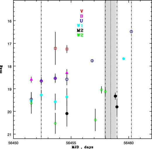
Swift/UVOT light curve during outburst rise in Aql X-1. The grey shaded band marks the time interval of hard/soft X-ray state transition. The state transition midpoint is shown by doted vertical line. Dot–dashed vertical lines correspond to time moments of broad-band SED measurements (see Section 5.1).
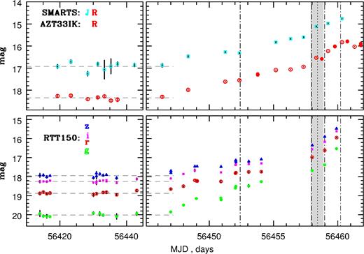
Optical–NIR light curves during the Aql X-1 quiescence (left-hand panels) and rise phase (right-hand panels) of major outburst in 2013 from RTT150, AZT33IK and SMARTS telescopes. The derived Aql X-1 quiescent fluxes in g, r, i, z, R and J bands are shown by horizontal dashed lines. The grey shaded band marks the time interval of hard/soft X-ray state transition. Dot–dashed vertical lines correspond to time moments of UVOT snapshot observations.
In order to measure the broad-band NUV–NIR spectral evolution during outburst rise time interval in Aql X-1, we chose four characteristic time moments, where observations from two instruments (Swift/UVOT–RTT150 or Swift/UVOT–SMARTS) were carried out quasi-simultaneously (within the time interval Δt ≲ 0.1d). These time moments are marked in Figs 1–3 by vertical dot–dashed lines (the corresponding broad-band NUV–NIR SEDs will be discussed in the Section 5.1 below).
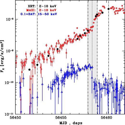
Orbit-averaged MAXI (2–10 keV) and Swift/BAT (15–50 keV) light curves are shown together with Swift/XRT light curve (in the 2–10 keV band). The midpoint and duration of hard/soft X-ray state transition are shown by doted vertical line and grey shaded band. Dot–dashed vertical lines correspond to time moments of broad-band SED measurements.
After the outburst detection in optical g΄, r΄, i΄, z΄ bands, the accretion activity of the source was soon confirmed by Swift/XRT follow-up observations (Degenaar & Wijnands 2013). The X-ray outburst happened to be among the brightest in soft X-rays among all Aql X-1 accretion events observed by MAXI or RXTE/ASM All Sky Monitors since 1997 (Güngör, Güver & Ekşi 2014). The overall morphology of this outburst in soft X-rays is characterized by a fast (∼10d) rise and a long (∼50d) decay. This type of curves are often observed in XN (Chen et al. 1997) and called FRED (Fast-Rise-Exponential-Decay). The FRED-type light curves in SXT are well qualitatively reproduced by standard Disc Instability Model, if effects of accretion disc evaporation and irradiation by the central source are taken into account (Dubus et al. 2001). The orbit-averaged light curves from MAXI (2 − 10 keV) and Swift/BAT (15 − 50 keV) for the Aql X-1 outburst rise phase are shown in Fig. 3. In the same figure, we show all available X-ray pointing measurements (in the same soft energy range 2–10 keV), carried out by Swift/XRT telescope during this interval.
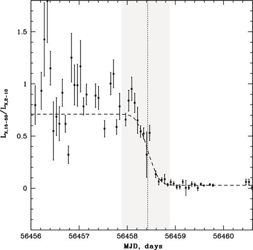
X-ray colour (15–50/2–10 keV) evolution around the hard/soft X-ray state transition interval during the rising part of Aql X-1 outburst. The grey shaded band shows the estimated time interval of state transition, the midpoint is shown by doted vertical line. The best-fitting model to X-ray colour evolution during state transition is shown by dashed line.
In our Swift/XRT observations, we are able to measure accurately only the soft fraction |$F_{\rm X,0.5{\rm -}10}$| of the total X-ray flux FX. The bolometric (0.5–100 keV) and hard (10–100 keV) X-ray flux can be estimated as: |$F_{\rm X} = f_{{\rm bol}} \cdot F_{\rm X,0.5{\rm -}10}$| and |$F_{\rm X,10{\rm -}100} = (f_{{\rm bol}}-1) \cdot F_{\rm X,0.5{\rm -}10}$|, where fbol means a bolometric correction coefficient. Note, that the bolometric correction is substantial for the spectrum in the hard X-ray state. To estimate fbol we used results from Sakurai et al. (2012), who analysed broad-band X-ray observations in the hard and soft X-ray states during Aql X-1 outburst in 2008 September–October, carried out by Suzaku observatory. By using their best-fitting models in Tables 2 and 3 (with fixed NH = 0.36 × 1022 cm−2), we calculated 0.5–10, 2–10, 15–50 keV and ‘bolometric’ 0.5–100 keV unabsorbed fluxes for the typical soft and hard X-ray state spectra. The estimated bolometric corrections are |$f^{{\rm hard}}_{{\rm bol}}=1.96$| and |$f^{{\rm soft}}_{{\rm bol}}=1.08$| for observational data points before and after X-ray state transition, respectively. In addition, we derived the FX,15–50/FX,2–10 ratio: 0.89 and 0.036 in the hard and soft state, respectively. As can be seen in Fig. 4, these values are well compared to the observed BAT/MAXI X-ray colours before and after state transition.
5 MODELLING THE BROAD-BAND SED EVOLUTION DURING OUTBURST RISE IN Aql X-1
5.1 SED measurements
There are two time moments before X-ray state transition midpoint and two time moments after, when we are able to measure a quasi-simultaneous (within ≲0.1d) broad-band SED of the source. Below we describe derived SED measurements and the fitting procedure in detail. Broad-band SED measurements during the outburst rise in Aql X-1:
t ≈ −6.02d. At this time moment, Swift/XRT and UVOT observations were carried out quasi-simultaneously with SMARTS telescope (t = −6.08d), and we combined these data to construct broad-band SED. Additionally, as can be noted (see Figs 1 and 2), the subsequent Swift/UVOT observation at t = −4.80d shows the same (within uncertainties) NUV fluxes. Thus, we included this Swift/UVOT observation and RTT150 observation carried out in between at t = −5.35d into the combined SED. The derived SED is shown in Fig. 5 (left-hand panel), where all the ‘non-simultaneous’ data points from RTT150 and the second Swift/UVOT observation are shown by open symbols.
t ≈ −0.46d. This time moment immediately before state transition, when Swift/UVOT W2-band observation at t = −0.46d was carried out quasi-simultaneously with RTT150 (t = −0.42d). As the previous Swift/UVOT observation at t = −0.79d shows the same (within uncertainties) W2 flux, we decided to include it into the combined SED. The resulting SED is shown in Fig. 5 (central panel), the ‘non-simultaneous’ Swift/UVOT data point is shown by open symbol.
t ≈ +0.55d. This is the most interesting SED measurement, we obtained it immediately after hard/soft X-ray state transition, the time moment of Swift/UVOT M2-band observation was carried out quasi-simultaneously with RTT150 (t = +0.56d). As the previous Swift/UVOT observation at t = +0.41d shows the same (within uncertainties) M2 flux, we decided to include it into the combined SED. The resulting SED is shown in Fig. 5 (central panel), where the ‘non-simultaneous’ Swift/UVOT data point is shown by open symbol.
t ≈ +1.80d. This is the final SED measurement we obtained near the outburst maximum in X-rays (see Fig. 3). The Swift/UVOT U-band observation was carried out quasi-simultaneously with SMARTS (t = +1.91d). The resulting SED is shown in Fig. 5 (right-hand panel).
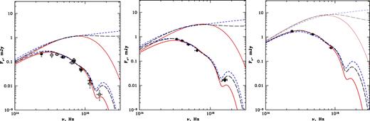
SED measurements (i) (left-hand panel), (ii) (central panel) and (iii) (right-hand panel), carried out at time moments t = −6.02d, −0.46d and +1.8d (with respect the middle of X-ray state transition). Best-fitting spectral models are shown by solid (blackbody), dashed (non-irradiated disc) and long dashed (disc with irradiation, C = 2.9 × 10⁻³) lines. Absorbed and unabsorbed curves for each model are shown by thick and thin lines, respectively. All model curves are smoothed with top-hat window Δλ/λ = 0.25 for better visual comparison with observations (see text). Note that best-fitting accretion rate for the non-irradiated disc model is always higher than |$\skew3\dot{M}_{\rm out}$| for the model with irradiation, and irradiated models show UV deficiency with respect to best-fitting models without irradiation.
The SED fitting procedure was performed in xspec package (Arnaud 1996), which provides a framework to compare various theoretical spectral models with observed spectra (primarily in the X-ray domain). xspec can be successfully used to fit spectral data from IR/Optical/UV observations (Arnaud 2010). We converted all NUV, Optical and NIR photometric measurements into pha-files using procedure flx2xsp from ftools package. For all filters, responses were defined by flat transmission curves with parameters λeff and Δλ (FWHM) (see Table 4). We note that the observed fluxes contain Aql X-1 counterpart and nearby 0.48 arcsec interloper star for ground-based Optical–NIR observations, and all nearby stars within 5 arcsec aperture for Swift/UVOT observations. In order to investigate the spectral evolution of Aql X-1 counterpart in outburst, we subtracted the corresponding flux levels measured during the time interval of Aql X-1 quiescence (see Table 4).
The interstellar extinction in photometric filters was calculated by using REDDEN model in xspec. This model utilize Cardelli et al. (1989) extinction law from far-IR to far-UV as a function of wavelength and of the parameter EB − V. For all spectral fits below, we adopted the fixed colour excess value EB − V = 0.65mag, as a best estimate for Aql X-1 (see Section 2).
5.2 Adopted spectral models
We tried to fit Aql X-1 NUV–NIR SEDs by two low-parametric spectral models:
Absorbed blackbody emission (REDDEN * BBODYRAD),
Absorbed emission from multicolour disc with possible X-ray irradiation (REDDEN * DISKIR).
Our choice of spectral models (A) and (B) is physically motivated. The simplified analytical picture of the non-stationary disc accretion during outburst rise phase in X-ray binaries was proposed in the work of Lyubarskij & Shakura (1987). The accretion disc development from the initial ring of matter can be divided into three characteristic stages:
– Formation of the disc from the initial ring of matter (‘torque’ formation stage).
– Quasi-stationary accretion with increasing accretion rate. At this stage a radially constant accretion rate is established in the inner regions of accretion disc. Near outer radii of the disc no changes from the initial mass distribution are expected and a transition zone is developed at intermediate radii. The region of quasi-stationary solution continuously expands as the transition zone moves outward.
– The accretion attenuation phase after the outburst maximum.
We are interested in stage 5.2, which could be potentially observed by our broad-band observations of outburst rise in Aql X-1 system. During this stage the mass distribution in the outer regions of the disc transforms from initial distribution (at the pre-outburst quiescence) into the stationary accretion disc (near the outburst maximum). Accordingly, the spectral evolution in the NUV–NIR range (which corresponds to emission from the outer parts of the disc) should transform from a single-temperature blackbody emitting ring into the multicolour (irradiated or non-irradiated) accretion disc emission. The initial ring of matter in the Lyubarskij & Shakura (1987) analytical model can be in reality a manifestation of the accretion disc with a surface density profile, highly concentrated to some outer radius – like Σ ∝ R1.14, which is supposed to form in the disc during the X-ray Nova quiescence (see Lasota 2001). The present numerical models of XN outbursts also show that the single-temperature emission remains at early stages of SXT outburst (see e.g. fig. 5 in Dubus et al. 2001). Note that, alternatively, a single blackbody model may correspond to the emission from the X-ray heated surface of companion star (if X-ray irradiation is strong enough) or a hot point, where a stream from L1-point meet the accretion disc. At the end of stage 5.2, the multicolour disc model corresponds to emission from the standard (Shakura & Sunyaev 1973) steady-state optically thick accretion disc with possible X-ray irradiation. The multicolour disc emission is expected to be established about the moment of the outburst maximum, the radial mass distribution in the disc at that moment does not depended on initial mass distribution in pre-outburst quiescence, see e.g. Lipunova (2015).
Thus, we expect that Model 5.2 should well describe NUV–NIR observations at the beginning of XN outburst (thermal emission from almost isothermal disc ring), and Model 5.2 should appear closer to the outburst maximum, when the automodel solution with constant mass accretion rate along the radius in the outer disc is established. As we will show in the Section 6.1, the observed spectral evolution during outburst rise in Aql X-1 qualitatively agrees with this theoretical picture. Below we describe the chosen spectral models and their parameters in detail.
Model (B). In order to model the irradiated accretion disc SED, we adopted the popular DISKIR7 model in xspec (without the inner disc coronal emission component, see Appendix A for details). The adopted model has three parameters: Tin,keV, logrout and fout (if irradiation is turned off – fout = 0). For a given X-ray luminosity illuminating the disc, these DISKIR parameters can be readily converted (see Appendix A – equations A4, A7 and A12) into physical parameters of the outer accretion disc–mass accretion rate |$\skew3\dot{M}_{\rm out}$|, disc outer radius Rout and the irradiation parameter C.
Further details about the standard irradiated disc Model 5.2 can be found in Appendix A.
5.3 ‘X-ray tomograph’ at the moment of hard/soft X-ray state transition in Aql X-1
The most remarkable moment at X-ray Nova outburst rise light curve is a hard/soft X-ray state transition. During the short-time interval ΔTh/s, the fast changes in the structure of the inner accretion flow (optically thin geometrically thick RIAF → optically thick geometrically thin standard Shakura–Sunyaev disc) are accompanied by a drastic softening of the X-ray spectrum: the amount of X-ray photons with E > 10 keV radically goes down. The temperature structure in the photosphere layers of the outer disc, which emit the observed NUV–Optical–NIR spectrum, can change substantially during the state transition interval, as it is directly governed by X-ray illumination (reprocessing time in the disc and its hot atmosphere for X-ray photons τrepr ≪ ΔTh/s, see τrepr estimates in Cominsky, London & Klein 1987; Mescheryakov, Revnivtsev & Filippova 2011b). The fast evolution of the X-ray spectrum at the moment of state transition, can serve as ‘X-ray tomograph’ to reveal the vertical structure and energy-depended X-ray heating efficiency of the outer accretion flow in XN. By using Aql X-1 SED measurements (ii)–(iii), carried out at the edges of hard/soft X-ray state transition interval, we will qualitatively test X-ray heating models for the outer accretion disc. Our methodology is outlined below.
In application to broad-band observations of Aql X-1, presented in this work, in Section 6.2 we will consider the following qualitative choices for X-ray heating of the disc during state transition interval: heating by bolometric, soft and hard X-ray flux with constant irradiation parameter.
- Fixed C model. Accretion disc is effectively heated by bolometric X-ray flux with constant irradiation parameter C, the irradiation heating Qirr(R) can be expressed asThis model was presented as Model 5.2 in the previous Section 5.2.(20)\begin{equation} Q_{{\rm irr}} = C \cdot \frac{D^2}{R^2} F_X . \end{equation}
- Fixed Cs model. In the case of disc irradiation solely by soft (0.5–10 keV) X-rays, the heating flux can be expressed byThe determination of model with ‘soft’ irradiation parameter Cs = const is justified in the case of direct illumination of the outer accretion disc by X-ray photons from the central source. Then soft X-rays with energies ≈2÷10 keV may play a primary role in the heating of the outer disc surface (see e.g. Suleimanov, Meyer & Meyer-Hofmeister 1999).(21)\begin{equation} Q_{{\rm irr}} = C_{\rm s} \cdot \frac{D^2}{R^2} F_{X,0.5{\rm -}10} . \end{equation}
- ‘Fixed Ch’ model. Disc heating solely by hard (10–100 keV) X-rays – in this case we getIf direct illumination of the disc surface is not possible for some reasons (e.g. due to concave disc height profile H ∝ R<1 or disc self-screening effect, see Dubus et al. 1999), then the hard (E ≳ 10 keV) X-rays, effectively scattered in the optically thin layers above the disc, may play a primary role in the disc irradiation heating (see e.g. Mescheryakov, Shakura & Suleimanov 2011a).(22)\begin{equation} Q_{{\rm irr}} = C_h \cdot \frac{D^2}{R^2} F_{X,10{\rm -}100} . \end{equation}
From parameters of DISKIR model (which we use for Aql X-1 SED fitting in xspec), one can easily derive the corresponding value of C, as well as Cs or Ch (by using equations A12 and A13 with replacement FX → FX, 0.5–10 or FX → FX, 10–100, respectively).
6 RESULTS
Four broad-band SED measurements (i)–(iv) were obtained during the Aql X-1 outburst rise phase (see Section 5.1) and were fitted by two spectral models 5.2 and 5.2, described in the Section 5.2 above. The best-fitting parameters for blackbody Model 5.2 and multicolour disc Model 5.2 with ( fout > 0) and without irradiation ( fout = 0) are presented in Table 5. The first three columns in Table 5 contain: time t with respect to state transition midpoint, orbital phase ϕ calculated from Aql X-1 ephemeris (see Table 1) and bolometric X-ray luminosity in Eddington units calculated in the following way: |$\frac{L_{\rm X}}{L_{\rm Edd}} = \frac{4\pi D^2 F_{\rm X,0.5{\rm -}10} f_{{\rm bol}}}{1.75\times 10^{38} \, \mathrm{erg\, s}^{-1}}$|, where the value of Eddington limit is taken for pure hydrogen composition and 1.4 M⊙ NS.
Aql X-1 SEDs best fits with REDDEN*BBODYRAD (Model 5.2) and REDDEN*DISKIR (Model 5.2) spectral models with fixed interstellar absorption EB − V = 0.65mag.
| #SED | ta | ϕb | LXc | A: | Tbbd | Kbbd | |$\chi _r^2$| | B: | kTine | logroute | foute | |$\chi _{\rm r}^2$| | |$\skew3\dot{M}_{\rm out}{}^f$| | Routf | Cf |
|---|---|---|---|---|---|---|---|---|---|---|---|---|---|---|---|
| (d) | LEdd | (eV) | 1011 | (d.o.f.) | (keV) | (10−3) | (d.o.f.) | |$\skew3\dot{M}_{\rm Edd}$| | Rtid | 10−3 | |||||
| (i) | −6.02 | 0.81 | 0.017 | 1.14±0.07 | 8.0±1.2 | 1.01 (11) | 1.91±0.04 | 4.85±0.08 | 0.0g | 2.17 (11) | 0.50±0.04 | |$0.61_{-0.09}^{+0.13}$| | 0 | ||
| 1.49±0.04 | 4.73±0.05 | 0.1g | 1.27 (11) | 0.18±0.02 | 0.46±0.05 | 2.9±0.3 | |||||||||
| 0.96±0.03 | 4.68±0.04 | 1.0g | 1.06 (11) | 0.031±0.004 | 0.41±0.04 | 4.9±0.6 | |||||||||
| (ii) | −0.46 | 0.90 | 0.20 | 1.10 | 17.8 | 11.7 (4) | 2.78 | 5.15 | 0.0g | 10.4 (4) | |||||
| |$2.05_{-0.18}^{+0.15}$| | 5.04±0.04 | |$0.07_{-0.03}^{+0.05}$| | 0.43 (3) | 0.66±0.21 | 0.94±0.08 | |$0.61_{-0.23}^{+0.44}$| | |||||||||
| (iii) | +0.55 | 0.13 | 0.33 | 0.81±0.03 | 79±7 | 2.76 (4) | 3.19 | 5.15 | 0.0g | 89.2 (4) | |||||
| 2.05g | 5.15 | 0.011 | 20.6 (4) | ||||||||||||
| 0.71 | 5.15 | 9.4 | 10.9 (3) | ||||||||||||
| (iv) | +1.80 | 0.71 | 0.50 | 1.07±0.03 | 66±5 | 0.38 (1) | 3.96 | 5.13 | 0.0g | 31.2 (1) | |||||
| 2.05g | 5.12±0.02 | 0.32±0.02 | 0.03 (1) | 0.66 | 1.14±0.05 | 1.11±0.08 |
Notes. Statistical errors on best-fit DISKIR model parameters and derived parameters are shown only if best-fitting model had goodness of the fit |$\chi ^2_r<5$|. All reported errors on parameters correspond to 1σ confidence level.
aTime with respect to X-ray state transition midpoint, t = T − Th/s.
bOrbital phase ϕ calculated from Aql X-1 ephemeris (see Table 1).
cEstimated bolometric 0.5–100 keV X-ray luminosity in Eddington units (see text, Section 6).
dBest-fitting parameters of REDDEN*BBODYRAD model with fixed EB − V = 0.65mag.
eBest-fitting parameters of REDDEN*DISKIR model with fixed EB − V = 0.65mag.
fPhysical parameters |$\skew3\dot{M}_{\rm out}$|, Rout, C of the irradiated disc Model 5.2 are derived from best-fitting DISKIR model parameters (see Appendix A).
gDISKIR parameters being fixed during the model fitting procedure.
All best-fitting spectral models, together with SED data points, are shown in Figs 5 and 6 by solid (blackbody), dashed (multicolour disc) and long dashed (multicolour disc with irradiation) lines. Both absorbed and unabsorbed curves for each model are shown (in Fig. 6 only one unabsorbed curve is shown for clarity). All spectral curves are smoothed with top-hat window Δλ/λ = 0.25 for better visual comparison with SED measurements, obtained in the broad-band filters having relative bandwidth in the range Δλ/λ = 0.14÷0.34 (see Table 4). The smoothing is primarily important on absorbed model curves in the NUV range, where model flux changes sharply with ν. We note that we derived smoothed model curves only for visualization purposes in Figs 5 and 6; all |$\chi ^2_r$| values presented in Table 5 were obtained in the xspec fitting framework. Below we discuss the derived results in detail.
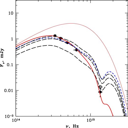
SED measurement (iii) at the time moment t = 0.55d (with respect the middle of X-ray state transition). Best-fitting blackbody and non-irradiated disc spectral models with fixed interstellar absorption EB − V = 0.65mag are shown by thick solid and short dashed lines, respectively. Unabsorbed blackbody model is shown by thin line. Thin long dashed lines show absorbed irradiated disc models with fixed irradiation parameter during X-ray state transition interval: Cs = 1.2 × 10⁻³ (upper curve), C = 6.1 × 10⁻⁴ (middle curve) and Ch = 1.25 × 10⁻³ (lower curve) – see description of these models in Section 6.2. All model curves are smoothed with top-hat window Δλ/λ = 0.25 for better visual comparison with observations.
6.1 Broad-band SED evolution during outburst rise in Aql X-1
First, we will consider SED measurements carried out during the Aql X-1 outburst rise in the hard X-ray state – (i), (ii) and SED obtained near the outburst maximum (iv). An interesting spectral evolution during the state transition interval [SEDs (ii)–(iii)] will be discussed in the next Section 6.2.
A first SED (i) was obtained from combination of quasi-simultaneous Swift/UVOT, SMARTS and RTT150 data (see Section 5.1) around a time moment t = −6.05d. As can be seen from Table 5 and Fig. 5 (left-hand panel), the blackbody model gives a substantially better fit than a multicolour disc model without irradiation. The best-fitting blackbody model with Tbb = 1.14 ± 0.07 eV and Kbb = (8.0 ± 1.2) × 1011 gives a goodness of the fit |$\chi ^2_r=1.01$| and best-fitting multicolour disc without irradiation gives |$\chi ^2_r=2.17$| (11 degrees of freedom), which rejects a later model with a p-value = 0.013. With inclusion of X-ray irradiation, the multicolour disc model fit can be improved significantly. For example, for Model 5.2 parameters C = (2.9 ± 0.3) × 10−3, |$\frac{\skew3\dot{M}_{\rm out}}{\skew3\dot{M}_{\rm Edd}}=0.18\pm 0.02$|, |$\frac{R_{\rm out}}{R_{{\rm tidal}}}=0.46\pm 0.05$| (which corresponds to best-fitting DISKIR model with fixed fout = 10−4, see Table 5) the goodness of the fit reaches |$\chi ^2_r=1.27$| (11 degrees of freedom). Note that |$C=2.9\times 10^{-3}\gg \frac{3{}G{}M_1{}\skew3\dot{M}_{\rm out}}{2{}L_{\rm X}{}R_{\rm out}}\approx 2.4\times 10^{-4}$| (see equation A9), thus the optical flux from the disc outer radius in this model is expected to be dominated by X-ray reprocessing. There is apparent degeneracy between irradiation parameter and accretion rate in the irradiated disc Model 5.2: by increasing C and decreasing |$\skew3\dot{M}_{\rm out}$|, one can obtain a slightly better fit to the data: e.g. C = 4.9 × 10⁻³, |$\skew3\dot{M}_{\rm out}\approx 0.031{}\skew3\dot{M}_{\rm Edd}$|, Rout ≈ 0.41Rtidal (which corresponds to best-fitting DISKIR model with fixed fout = 10−3, see Table 5) with the goodness of the fit |$\chi ^2_r=1.1$| (11 degrees of freedom). At this point one can conclude that both irradiated disc Model 5.2 and single blackbody Model 5.2 provide equally acceptable fits to the SED (i).
Estimates of correlation coefficients between NUV/Optical/NIR fluxes and 0.5–10 keV X-ray flux, measured during Aql X-1 early outburst rise in the hard X-ray state (time interval 56451.5–54454.6 MJD).
| Band | abf | P(>|abf|) | a0.025–a0.975 |
|---|---|---|---|
| (d−1) | (d−1) | ||
| Swift/UVOT | |||
| W2 | −0.7912±0.600 | 0.19 | −1.966–0.384 |
| W1 | 0.0174±0.268 | 0.95 | −0.508–0.543 |
| U | 0.3665±0.222 | 0.10 | −0.070–0.803 |
| B | 0.1567±0.133 | 0.24 | −0.104–0.417 |
| V | −0.0623±1.411 | 0.96 | −2.828–2.703 |
| RTT150 | |||
| g΄ | 0.2671±0.047 | <5 × 10⁻⁴ | 0.176–0.358 |
| r΄ | 0.0608±0.049 | 0.21 | −0.035–0.157 |
| i΄ | 0.0657±0.046 | 0.15 | −0.024–0.156 |
| z΄ | 0.0618±0.055 | 0.26 | −0.045–0.169 |
Note. Relations are fit by the power law, |$\log _{10}(F_{\rm band})=a \cdot {}\log _{10}(F_{\rm X,0.5{\rm -}10}) + b$|, where Fband corresponds to flux in g΄, r΄, i΄, z΄RTT150 or W2, W1, U, B, VSwift/UVOT filter, respectively, |$F_{\rm X,0.5{\rm -}10}$|–Swift/XRT interpolated X-ray flux (see text). We have derived best-fitting parameter abf and null-hypothesis (Fband = const) probability P(>|abf|) by using the linear regression statistical model (weighted least squares) implemented in the Statsmodels module (see https://github.com/statsmodels/statsmodels) for python. All errors correspond to one standard deviation. In the last column – derived P = 0.025 and P = 0.975 percentiles for correlation coefficient are shown.
As can be seen from Table 6, observational data for all filters except g΄ band are consistent with null-hypothesis of constant flux Fband = const during the considering time interval. The derived value of correlation coefficient for g΄ band (abf = 0.2671 ± 0.047) is substantially lower than expected for Optical–X-ray correlation |$F_{{\rm opt}}\propto {}F_X^{\approx 0.5}$| (van Paradijs & McClintock 1994). Correlation between g΄ band and X-rays is consistent with value a = 0.25, which is expected if this spectral band lies in the Rayleigh–Jeans part of the disc spectrum (it is definitely not the case for blue g΄ band). Note that abf estimates for other RTT150 filters (r΄, i΄, z΄) are well below the 0.25–0.5 interval expected for disc X-ray reprocessing.
Therefore, the lack of optical orbital variability and absence of expected Optical/X-ray correlation around t = −6.05d suggest that the SED (i) most probably is emitted by accretion flow without significant irradiation and with ∼ blackbody spectrum in the NUV–NIR spectral range. We note that blackbody emission from disc ring heated by viscous dissipation is expected at early stages of non-stationary disc accretion during X-ray Nova outburst rise (see Section 5.2). The relative width of the blackbody emitting disc ring at radius R can be estimated as
The next SED measurement (ii) was obtained just before hard/soft X-ray state transition at t = −0.43d. Neither blackbody (|$\chi ^2_r=11.7$|, 4 degrees of freedom), nor multicolour disc without irradiation (|$\chi ^2_r=11.0$|, 4 degrees of freedom) provide an acceptable fit for this SED measurement, but it can be well described (|$\chi ^2_r=0.43$|, 3 degrees of freedom) by the irradiated multicolour disc Model 5.2 with reliable parameters: |$\skew3\dot{M}_{\rm out}/\skew3\dot{M}_{\rm Edd}=0.66\pm 0.21$|, Rout/Rtidal = 0.94 ± 0.08 and |$C=6_{-2}^{+4}\times 10^{-4}$|.
The final SED measurement (iv) was carried out at a time moment t = +1.8d near the X-ray outburst maximum. As can be seen from Table 5, the multicolour disc without irradiation is statistically unacceptable model for this SED. Both irradiated multicolour disc or single-temperature blackbody models provide good fit to the SED data points. We note that there are only three flux measurements (J, R, U bands) combined in this SED, and NUV flux (M2/W2 bands at ∼2000 Å) measurement is not available at this time moment. We expect a degeneracy between physical parameters |$\skew3\dot{M}$| and C in the Model 5.2. Therefore, we decided to fix a mass accretion rate during the fit, to the reasonable value estimated for the SED (ii) (at t = −0.46d). The Model 5.2 with fixed |$\skew3\dot{M}_{\rm out}=0.66\, \skew3\dot{M}_{\rm Edd}$| provides an acceptable fit with |$\chi ^2_r=0.03$| (1 degrees of freedom) with a best-fitting parameters C = (1.1 ± 0.1) × 10−3 and |$\frac{R_{\rm out}}{R_{{\rm tidal}}}=1.14\pm 0.05$| (see Table 5 and Fig. 5 right-hand panel). From numerical simulation of outbursts in XN (see e.g. fig. 5 in Dubus et al. 2001) it is expected that multicolour disc SED is already established at the moment of outburst maximum. Therefore, we also may prefer the irradiated multicolour disc as a best model for the SED (iv).
In sum, we make a conclusion that the observed SED evolution (i), (ii), (iv) during outburst rise in Aql X-1 can be well understood as thermal emission from non-stationary accretion disc flow with radial temperature distribution transforming from ∼ single-temperature blackbody emitting ring (heated primarily by viscous dissipation) at early stages of outburst into the multicolour irradiated accretion disc measured close to the X-ray outburst maximum.
6.2 Evolution of the broad-band SED during the hard/soft X-ray state transition in Aql X-1
X-ray state transition interval during outburst rise in Aql X-1 is covered by two SED measurements (ii) and (iii) at time moments t = −0.46d and +0.55d, luckily carried out quasi-simultaneously (within time interval <0.05d) by Swift/UVOT and RTT150 telescopes (see Section 5.1). As it was discussed above in Section 6.1, the SED (ii) (at the start of X-ray state transition) can be well fitted by Model 5.2 with reasonable physical parameters of the irradiated accretion disc: mass accretion rate |$\skew3\dot{M}_{\rm out}/\skew3\dot{M}_{\rm Edd}=0.66\pm 0.21$|, outer radius Rout/Rtidal = 0.94 ± 0.08 and irradiation parameter |$C=6_{-2}^{+4}\times 10^{-4}$|. By having in mind theoretical considerations presented in Section 5.3, one may expect that this irradiated disc model can also provide a good approximation to SED (iii) measured at the end of X-ray state transition interval. Let us consider, what we see in reality.
As it is shown in Table 5, surprisingly, multicolour disc Model 5.2 with or without irradiation does not provide an acceptable fit to the SED (iii) for any choice of model parameters. For example, best non-irradiated disc model has |$\chi ^2_r=89.2$| (4 degrees of freedom), this model is shown in Fig. 6 by short dashed line (only absorbed model is shown). Allowing irradiation in the Model 5.2 only slightly improves a goodness of the fit. For the fixed DISKIR temperature parameter Tin = 2.05 keV [which corresponds to fixed |$\skew3\dot{M}_{\rm out}=0.66\cdot \skew3\dot{M}_{\rm Edd}$| as for SED (ii)] best fit shows goodness value |$\chi ^2_r=20.59$| (4 degrees of freedom). Making Tin (and |$\skew3\dot{M}_{\rm out}$| respectively) also a free parameter, gives a best-fitting with |$\chi ^2_r=10.9$| (3 degrees of freedom), see Table 5. Thus, we can conclude that multicolour disc Model 5.2 is unacceptable for SED (iii). From the other hand, a single-temperature blackbody Model 5.2 gives a much better fit to SED (iii) with best-fitting parameters: Tbb = 0.81 ± 0.03 eV, Kbb = (79 ± 7) × 1011 (|$\chi ^2_r=2.76$|, 4 degrees of freedom). Best-fitting absorbed and unabsorbed blackbody models are shown in Fig. 6 by thick and thin solid lines, respectively. Note, if we exclude the second Swift/UVOT data point (which was carried out not fully simultaneously with RTT150 observation, see Section 5.1) from consideration, then the best-fitting blackbody Model 5.2 with Tbb = 0.76 ± 0.03 eV and Kbb = (91 ± 9) × 1011 became fully statistically acceptable with the goodness of the fit equal to |$\chi ^2_r=0.83$| (3 degrees of freedom). One can conclude that at the end of X-ray state transition in SXT Aql X-1, the blackbody like SED in the NUV–NIR spectral range (2000–9000 Å) is established.
As can be seen in Figs 1 and 2, fluxes in different NUV–NIR bands clearly show a different rise rates during the hard/soft X-ray state transition interval. The measured flux ratio between observation (iii) and (ii) rises with increasing filter effective wavelength: 0.86 ± 0.15 (W2/M2 band, λeff ≈ 2000 Å), 1.32 ± 0.05 (g΄ band, λeff = 4715 Å), 1.39 ± 0.06 (r΄ band, λeff = 6182 Å), 1.43 ± 0.06 (i΄ band, λeff = 7592 Å) and 1.51 ± 0.07 (z΄ band, λeff = 9003 Å).
- Fixed C model. In order to better understand the NUV–NIR spectral evolution during X-ray state transition, we calculated expected SED for the time moment t = +0.55d according to model of irradiated disc heated by bolometric X-ray flux, with physical parameters |$\skew3\dot{M}_{\rm out}=0.66\cdot \skew3\dot{M}_{\rm Edd}$|, Rout = 0.94 · Rtid and C = 6.1 × 10⁻⁴, which correspond to DISKIR model parameters: kTin = 2.05 keV, logrout = 5.04, fout = 0.69 × 10⁻⁴ at t = −0.46d [a best-fitting model for SED (ii), see above] and kTin = 2.05 keV, logrout = 5.04, fout = 1.14 × 10⁻⁴ at t = +0.55d. Note that for fixed irradiation parameter C (see equation A13), we rescale fout parameter of DISKIR model aswhere FX(−0.46d) and FX(+0.55d) correspond to bolometric 0.5–100 keV X-ray flux estimated at the beginning and at the end of X-ray transition interval, respectively. The derived model SED (with applied interstellar absorption EB − V = 0.65mag) for the time moment t = +0.55d is shown in Fig. 6 by long dashed (middle) line. As can be seen from this figure, at the time moment t = 0.55d the irradiated disc model (with constant |$\skew3\dot{M}$|, Rout, C over the state transition interval) underestimate/overestimate the observed flux in the NIR/NUV spectral bands, respectively.(25)\begin{equation} f_{\rm out}(+0.55^d)= f_{\rm out}(-0.46^d)\frac{F_{\rm X}(+0.55^d)}{F_{\rm X}(-0.46^d)} , \end{equation}
Fixed Cs model. Irradiated disc model with |$\skew3\dot{M}_{\rm out}=0.66\cdot \skew3\dot{M}_{\rm Edd}$|, Rout = 0.94 · Rtid, heated by soft 0.5–10 keV X-rays with fixed ‘soft’ irradiation parameter Cs = 1.2 × 10⁻³. The corresponding DISKIR model has parameters: kTin = 2.05 keV, logrout = 5.04, fout = 0.69 × 10⁻⁴ at t = −0.46d and fout = 2.06 × 10⁻⁴ at t = +0.55d, respectively. Note that for fixed Cs (see equation A13), the DISKIR parameter fout was rescaled according to equation (25) with appropriate replacement: FX → FX,0.5–10. The derived absorbed model SED at t = +0.55d is shown in Fig. 6 by long dashed (upper) line.
Fixed Ch model. Irradiated disc model with |$\skew3\dot{M}_{\rm out}=0.66\cdot \skew3\dot{M}_{\rm Edd}$|, Rout = 0.94 · Rtid, heated by hard 10–100 keV X-rays with fixed ‘hard’ irradiation parameter Ch = 1.25 × 10⁻³. The corresponding DISKIR model has parameters: kTin = 2.05 keV, logrout = 5.04, fout = 0.69 × 10⁻⁴ at t = −0.46d and fout = 0.172 × 10⁻⁴ at t = +0.55d, respectively. For Ch = const, the DISKIR parameter fout was rescaled according to equation (25) with replacement FX → FX,10–100. The derived absorbed model SED at t = +0.55d is shown in Fig. 6 by long dashed (lower) line.
From Fig. 6 one can see that the observed Aql X-1 flux evolution in the NIR (∼z΄ band) can be described by accretion disc heated by soft X-ray photons (‘fixed Cs’ model, see above) and the flux evolution in the NUV (W2/M2 band) can be described by the accretion disc heated by hard X-ray photons (‘fixed Ch’ model). Note that ∼1d later (at the time moment t = 1.8d), Aql X-1 brightness in all measured NUV–NIR filters increase significantly, with the biggest relative flux rise detected in the NUV. Thus, the relative rise of NUV brightness in the time interval t = 0.55–1.8d makes the form of observed SED similar to our expectations for irradiated disc model.
We think that the observed Aql X-1 broad-band spectral evolution during the X-ray state transition can be understood if one considers a different mechanism of X-ray heating for NUV- and NIR-emitting regions of the disc. Let us suppose that NUV-emitting regions in the disc are heated primarily by scattered (in the hot corona or wind formed above the optically thick accretion flow, see e.g. Mescheryakov et al. 2011a) hard (E > 10 keV) X-ray photons, due to:
possible screening of NUV-emitting disc regions from direct X-ray photons from the central source around the moment of X-ray state transition or/and
possible photoabsorption of soft X-ray photons for these regions predominantly in the atmosphere layers of the disc, far above the thermalization depth.
7 CONCLUSIONS
We studied a time evolution of the broad-band (NUV–Optical–NIR) SED in NS X-ray Nova Aql X-1 during the rise phase of a bright FRED-type outburst in 2013. By using quasi-simultaneous observations from Swift orbital observatory and RTT150, AZT33IK, SMARTS 1-m class optical telescopes, we show that evolution of broad-band SED can be understood in the framework of thermal emission from non-stationary accretion disc, which radial temperature distribution transforms from a single blackbody emitting ring at early stages of outburst into the standard multicolour irradiated accretion disc, with irradiation parameter C ≈ 6 × 10⁻⁴, measured at the end of hard X-ray state and near the outburst maximum.
By using photometric observations, carried out exactly at the edges of X-ray hard/soft state transition interval, we find an interesting effect: a small decrease in NUV flux during this time interval is accompanied by flux rise in NIR–Optical bands. The NUV flux decrease correlates with the hard X-rays E > 10 keV drop during the X-ray state transition, and the Optical–NIR flux rise correlates with the soft X-rays rise during the same time interval. In our interpretation, at the moment of X-ray state transition in Aql X-1 the UV-emitting parts of the accretion disc are screened from direct X-ray photons from the central source and heated primarily by hard X-rays, effectively scattered in the hot corona or wind formed above the optically thick accretion flow. At the same time, the outer and colder regions of accretion disc, emit in the Optical–NIR and are primarily heated by direct X-ray illumination.
We point out that simultaneous multiwavelength observations during the fast X-ray state transition interval in provide an effective tool to directly test the energy-dependent X-ray heating efficiency, vertical structure and accretion flow geometry in the outer regions of accretion disc in XN.
Acknowledgements
Authors are grateful to the anonymous referee for critical comments.
AVM is deeply thankful to Mike Revnivtsev, a great academic advisor, professional team leader as well as a distinguished colleague, who sadly passed away too soon.
AVM and NIS acknowledge support through the Russian Scientific Foundation grant 14-12-00146 for the main results of this research covering Aql X-1 SED evolution modelling and interpretation (Sections 5 and 6). AVM also acknowledges a partial support of the Russian Government Program of Competitive Growth of Kazan Federal University (for results presented in Section 4). IMKh, IFB and MNP thank to TUBITAK, IKI, KFU and AST for partial supports in using RTT150 (Russian-Turkish 1.5 m telescope in Antalya), which made our RTT150 observational monitoring program of Aql X-1 possible. ST acknowledges a partial support through RFBR project 17-52-80139 BRICS-a (for Swift/XRT and Swift/UVOT data reduction presented in Section 3). Experimental data from AZT33IK telescope were recorded by the Angara Multiaccess Center facilities at ISTP SB RAS. This paper has made use of up-to-date SMARTS optical/near-infrared light curves that are available at www.astro.yale.edu/smarts/xrb/home.php. This research has made use of the MAXI data provided by RIKEN, JAXA and the MAXI team, and Swift/XRT and BAT data obtained from the High Energy Astrophysics Science Archive Research Center of NASA. AVM is thankful to the Swift PI, Neil Gehrels, for accepting our requests for ToO observations of Aql X-1 with Swift/XRT.
Facilities:Swift/XRT, Swift/BAT, MAXI, RTT150, AZT33IK, SMARTS.
Swift Helpdesk private communication.
REFERENCES
APPENDIX A: Measuring physical parameters of irradiated accretion disc by using DISKIR spectral model
Gierliński et al. (2009) build a simple model for Optical/UV emission from the stationary |$\skew3\dot{M}(R)={\rm const}$| multicolour disc self-irradiated by inner parts of the disc and coronal emission in black hole binaries. The model DISKIR became publicly available among other additive models in xspec package. We adopted this model to fit NUV–Optical–NIR SED of NS X-ray Nova Aql X-1.
The DISKIR model has nine parameters:
Tin,keV(keV), innermost temperature of the unilluminated disc in units (keV),
γ, asymptotic power-law photon index,
Te,keV, electron temperature (high-energy rollover) in units (keV),
Lc/Ld, ratio of luminosity in the Compton tail to that of the unilluminated disc,
fin, fraction of luminosity in the Compton tail which is thermalized in the inner disc,
rirr, radius of the Compton illuminated disc in terms of the inner disc radius,
fout, fraction of bolometric flux which is thermalized in the outer disc,
logrout, log 10 of the outer disc radius in terms of the inner disc radius,
- Normalization parameter (as in diskbb model):where Rin is the inner disc radius in (cm), D5 is the distance in units 5 kpc, i is the system inclination.(A1)\begin{equation} K=4\times 10^{-10}\left(\frac{R_{\rm in}}{D_5}\right)^2{}\cos (i) , \end{equation}
Among all parameters of the model, we are interested only in four of them (which define disc SED in the NUV–NIR spectral range): K, Tin,keV, logrout and fout. Other parameters were fixed to their default values: γ = 1.7, kTe,keV = 100, fin = 0.1, rirr = 1.2 and Lc/Ld = 0 – irradiation of the inner disc and coronal emission are turned off. By using equations from Gierliński et al. (2009) (see their section 3) parameters K, Tin,keV, logrout, fout can be converted into the physical parameters we are interested.
