


Abstract
We present a novel strategy to uncover the Galactic population of quiescent black holes (BHs). This is based on a new concept, the photometric mass function (PMF), which opens up the possibility of an efficient identification of dynamical BHs in large fields-of-view. This exploits the width of the disc H α emission line, combined with orbital period information. We here show that H α widths can be recovered using a combination of customized H α filters. By setting a width cut-off at 2200 km s−1 we are able to cleanly remove other Galactic populations of H α emitters, including ∼99.9 per cent of cataclysmic variables (CVs). Only short-period (Porb <2.1 h) eclipsing CVs and AGNs will contaminate the sample but these can be easily flagged through photometric variability and, in the latter case, also mid-IR colours. We also describe the strategy of a deep (r = 22) Galactic plane survey based on the concept of PMFs: HAWKs, the HAlpha-Width Kilo-deg Survey. We estimate that ∼800 deg2 are required to unveil ∼50 new dynamical BHs, a three-fold improvement over the known population. For comparison, a century would be needed to produce an enlarged sample of 50 dynamical BHs from X-ray transients at the current discovery rate.
1 INTRODUCTION
The historic discovery of gravitational waves (GW) from merging black holes (BHs) has undoubtedly opened a new era in astronomy (Abbott et al. 2016a,b). It means that BHs can now be detected without an electromagnetic counterpart. Also, the prediction of ∼103 new merging BHs to be discovered by Advanced LIGO in the next decade will allow for the first BH demographic studies across cosmological times (Abbott et al. 2016c; Kovetz et al. 2017; Sesana 2016; Cholis 2017; Elbert, Bullock & Kaplinghat 2017). Different formation scenarios, however, have been proposed to explain the GW events GW150914 and GW151226, including massive binaries at low metallicity, dynamical encounters in globular clusters or primordial BHs (Belczynski et al. 2016; Coleman Miller 2016; De Mink & Mandel 2016; Rodriguez, Chatterjee & Rasio 2016; Clesse & García-Bellido 2017). At present, it is unclear which model can better accommodate the new GW BHs and it seems likely that a degenerate combination of multiple formation channels may be responsible for the entire population. In this context, the study of BHs in Galactic X-ray binaries remains extremely valuable because they present us with a homogeneous reference sample, drawn from a very specific formation channel in solar metallicity environment (e.g. Wang, Jia & Li 2016, and references therein). This is precisely the scope of the current paper.
Galactic BHs are mostly discovered in X-ray transients (XRTs), a subclass of X-ray binaries which exhibit episodic outbursts triggered by accretion disc instabilities (see e.g. Belloni, Motta & Muñoz-Darias 2011). These X-ray brightenings can be dramatic as they happen within a day or so, and can often outshine the brightest sources in the sky, making them easy to spot by X-ray monitoring satellites. But between these extraordinary outbursts, BH XRTs hibernate in a ‘quiescent’ state, which can last for several decades or more, with typical X-ray luminosities below ∼1032 erg s−1. It is during these times that it becomes possible to detect the faint low-mass donor star at optical/NIR wavelengths and exploit its kinematics to constrain the masses of the binary components. About 60 XRTs with suspected BHs (as indicated by their X-ray timing and spectral properties) have been discovered since the dawn of X-ray astronomy but most of them faded below the detection threshold of present instrumentation during their decay (Corral-Santana et al. 2016). Time-resolved spectroscopy in quiescence is required for dynamical confirmation (i.e. a mass function greater than ∼3 M⊙) and this has only been achieved in ∼50 years for 17 BH transients (Casares & Jonker 2014). For detailed population studies it is therefore critical to dramatically increase the number of dynamical BHs in X-ray binaries. This requires a new research methodology rather than simply waiting for new transients to trigger an outburst, as this would take many decades to barely double the current number.
In this regard, lessons can be learned from the study of supermassive BHs in quasars (QSOs) and active galactic nuclei (AGNs). Nearby supermassive BHs are also weighed from the kinematics of central stars or, in exceptional circumstances, water radio masers. However, in distant galaxies, when the BH radius of influence cannot be resolved, empirical scalings with galaxy properties (such as the MBH–σ relation in the bulge and others based on reverberation mapping of the broad-line region, BLR) have to be applied (see Kormendy & Ho 2013 for a review of the different methods). In the most frequent form of reverberation-based techniques, the BH mass scales with the width of emission lines formed in the BLR and the continuum luminosity, a proxy for the BLR size (Peterson et al. 2004; Vestergaard & Peterson 2006). Similarly, when the donor star is not detected in quiescent XRTs, scaling relations of spectral features with fundamental binary parameters may prove useful. For example, in Casares (2016) (hereafter Paper II), we show that the ratio between the double-peak separation and the full width at half-maximum (FWHM) of the H α line, formed in the accretion disc, correlates with the binary mass ratio q = M2/M1 for q ≲ 0.25 (with M2 and M1 being the masses of the companion and BH, respectively). This stems from the fact that the double-peak separation traces the outer disc truncation radius which, for these extreme mass ratios, is determined by the 3:1 resonance tide with the companion star. The relation presented in Paper II can, for instance, provide a first estimate of the BH mass when M2 is inferred from broad-band colours or the orbital period (assuming the companion is a Roche lobe filling Main Sequence star dominating the quiescent optical/NIR spectrum).
As a matter of fact, equation (1) proves very useful to study faint XRTs: it simply requires resolving the width of the H α line (usually the strongest feature in the spectrum) rather than measuring the Doppler shifts of weak absorption lines from the donor star in phased-resolved spectra. Therefore, if the orbital period is known (e.g. through photometric variability) then mass functions can be extracted from single-epoch spectroscopy. This effectively allows extending dynamical studies to XRTs ∼2 mag fainter than is currently possible, anticipating what 40-m class telescopes can achieve in the next decade using traditional techniques. Examples of this strategy are presented in Zurita, Corral-Santana & Casares (2015), Mata-Sánchez et al. (2015) and Torres et al. (in preparation); see also Paper II.
In this paper we present a proof-of-concept on how H α FWHMs can be measured through photometry using custom interference filters, and how this can be exploited to filter out contaminating sources that plague classic H α surveys (Section 2). In Section 3 we propose a survey strategy to identify hibernating BHs from H α widths and PMF selection. Finally, in Sections 4 and 5 we discuss our results and summarize the conclusions. We envision that this new methodology has the potential for boosting the statistics of dynamical BHs by an order of magnitude within only a few years.
2 A PHOTOMETRIC SYSTEM TO MEASURE H α WIDTHS
Dormant BH XRTs are very difficult to identify because of their extremely low accretion luminosities. In turn, the companion (typically a K-type star) dominates the optical spectrum, thereby effectively disguising quiescent XRTs amongst the myriad of field stars. Only the presence of superimposed broad emission lines from the accretion disc, most notably H α, can betray their presence. In fact, current H α surveys of the Galactic plane, such as the SuperCOSMOS H-alpha Survey (SSH; Parker et al. 2005) or the INT Photometric H α Survey of the Northern Galactic Plane (IPHAS; Drew et al. 2005) might contain quiescent BHs but, unfortunately, they are vastly outnumbered by other populations of H α emitters such as symbiotic binaries, CVs, Be stars or planetary nebulae. For example, among ∼104 H α sources contained in IPHAS (Drew et al. 2005; Witham et al. 2008) no BH candidates have yet been produced. Another approach, followed by the Galactic Bulge Survey (GBS), relies mainly on cross-matching H α emitting objects with weak X-ray sources from a shallow Chandra survey of the Galactic bulge (Jonker et al. 2011, 2014). About 25 new quiescent BHs were predicted by GBs but only intervening CVs (mostly magnetic), W UMa or coronally active stars have been securely identified so far (e.g. Torres et al. 2014; Wevers et al. 2017).
Here, we propose a new route that exploits the width of the H α line as a tracer of the strong gravitational field exclusive to BHs. From the compilation presented in Paper I we note that quiescent BHs typically possess FWHM ≳ 1000 km s−1, i.e. much larger than observed in most other populations of H α emitters. Therefore, in order to flush out potential contaminants it would be of great interest to develop a photometric system tailored to measure H α line widths. In principle, this could be achieved with just a pair of H α interference filters: one sufficiently broad to contain the entire line flux (hereafter called H α broad, H αb) and another filter matched to sample only the line core (H α narrow, H αn). To test this idea we have simulated a pair of H αb and H αn filters by scaling filter 197 from the Wide Field Camera (WFC) on the 2.5-m Isaac Newton Telescope (INT), which has an effective FWHM of 95 Å.2 The two simulated filters have been shifted to the H α rest wavelength i.e. 6562.76 Å. For the H αb filter we take a bandwidth of 150 Å so as to encompass the entire flux of the broadest BH H α line currently known, i.e. that of Swift J1357−0933 (Paper I). Regarding the H αn filter we start by adopting a bandwidth of 33 Å (=1508 km s−1). In addition, we have produced a set of synthetic ‘interacting binary’ spectra consisting of double-peaked H α profiles with fixed EW = 50 Å (we take EWs of emission lines as positive henceforth.) and FWHM = 670–4450 km s−1 sitting on a reddened linear continuum (Appendix A). In the top panel of Fig. 1 we present the synthetic spectra, together with the transmission curves of the simulated filters.
Top: synthetic double-peaked H α spectra with FWHM = 670–4450 km s−1, together with the transmission curves of our simulated H α filters. Bottom: variation of the filter's flux ratio versus FWHM. The flux ratio is computed through the convolution of the synthetic spectra with the H α filters.
The synthetic spectra were convolved with the transmission curves of the H αb and H αn filters and integrated over wavelength to derive associated fluxes (Appendix A). Here and henceforth, we sample the filter's response curves and the spectra to a common wavelength scale of 1 Å pixel−1. The bottom panel in Fig. 1 displays the ratio of fluxes obtained from the pair of H α filters as a function of line FWHM. The latter was derived through fitting Gaussian functions to the synthetic profiles (see Appendix A). The smooth curve indicates that FWHM values can indeed be recovered from the combined fluxes provided by the simulated filters. We subsequently applied the same exercise to a sample of flux-calibrated spectra of BHs and CVs from the compilation presented in Paper I3 and the result is presented in Fig. 2. This time the smooth trend is replaced by significant scatter, caused by large variations in line EW from system to system. This can be interpreted as the effect of different underlying continua diluting the contribution of the line to the total flux. In other words, a broad emission line sitting on a strong continuum can mimic the same flux ratio as a narrow line over a weak continuum. Therefore, in order to measure accurate line widths it is crucial to know the EW of the line beforehand and this can be accomplished with an extra observation using a broader filter (r band hereafter), also centred at H α.
Same as Fig. 1 but for a sample of nine BH (filled circles) and four CV (open circles) real spectra. Error bars in the lower panel are smaller than the symbol size and are not displayed. The dotted line indicates the trend derived from synthetic spectra, with EW = 50 Å.
2.1 Photometric EWs
Top: synthetic double-peaked H α spectra with FWHM = 2500 km s−1 and different EWs in the range 10–250 Å, together with the transmission curves of our simulated H αb and r-band filters. Bottom: Photometric EWs (EWph), as extracted from equation (3) with C1 = 1.155, versus model EWs. The dotted line represents EWph = EW.
2.2 Photometric FWHMs
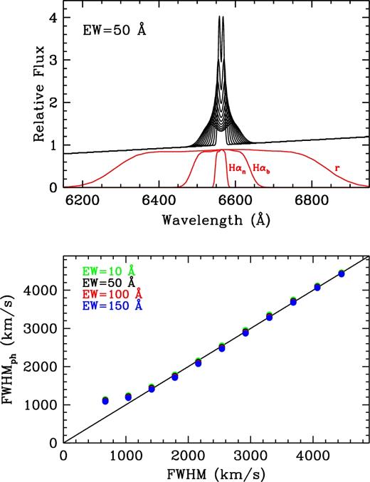
Top: example synthetic double-peaked H α spectra with EW = 50 Å and FWHM in the range 670–4450 km s−1, together with the transmission curves of our simulated H αn, H αb and r-band filters. Bottom: Photometric FWHMs (FWHMph), as provided by equation (4) with C2 = 0.826, versus FWHMs measured through a Gaussian fit for different model EWs in the range 10–150 Å. The dotted line represents FWHMph = FWHM. Note that only spectra with FWHM ≤ 1200 km s−1 deviate from the line because their widths are smaller than the bandwidth of the narrow H α filter.
A final test is performed with our previous sample of real BH and CV spectra and the results are presented in Fig. 5. In contrast to Fig. 2, the variations in line EW are now accounted for, allowing us to recover line widths at <5 per cent accuracy for FWHM ≥ 1200 km s−1. Here, 5 per cent indicates the largest fractional difference between the true data FWHM and the FWHMph values provided by equation (4). Therefore, photometric observations with a combination of only three filters (broad-band r plus two narrow-band H α filters) are sufficient to determine the width (and equivalent width) of the H α line in quiescent BH XRTs.
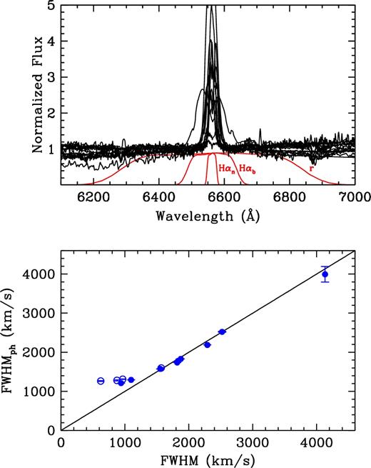
Same as Fig. 4 but for a sample of nine BHs (filled circles) and four CVs (open circles). Error bars in the lower panel are smaller than the symbol size in all but one case. Photometric widths recover real FWHMs to better than 5 per cent for FWHM ≥ 1200 km s−1.
2.3 Width cut-off for BH selection
Having proved that line FWHMs can be reliably measured with our photometric system we now need to define an optimal width cut-off to efficiently select quiescent BHs. This is an important issue as it determines the fraction of other H α emitting objects that will be rejected. Larger cut-off widths will filter out narrow H α emitters but also BHs at lower inclinations and, therefore, a compromise must be devised. For example, a cut-off at FWHM ∼ 1500 km s−1 will instantly clean out most potential contaminants such as T Tau, Be stars, chromospherically active stars or planetary nebulae. Only CVs at moderately high inclinations can produce H α lines this broad because of the deep potential wells of their accreting white dwarfs. However, with a Galactic density of ∼104 kpc−3 (Pretorius & Knigge 2012; see also Burenin et al. 2016 for an update based on recent constraints on the X-ray luminosity function) CVs are a factor of ≈103 more numerous than BH XRTs (e.g. Corral-Santana et al. 2016) and most likely will dominate the Galactic population of H α contaminants, even at these large widths. So, it is important to set a more stringent width cut-off in order to optimize the rejection of potentially contaminating CVs.
To investigate this issue we have run Monte Carlo simulations (105 trials) of the expected distribution of FWHMs for the two binary populations. In the case of BH XRTs we have computed FWHMs from equation (2), assuming an isotropic distribution of inclinations, i.e. 〈cos i〉 = 0.5. Following Özel et al. (2010) we have drawn BH masses from a normal distribution with mean 7.8 M⊙ and σ = 1.2 M⊙. Porb and q values are also obtained from normal distributions with 〈Porb〉 = 0.287 d, σ(Porb) = 0.14, 〈q〉 = 0.05 and σ(q) = 0.02. These have been parametrized from Gaussian fits to the observed distributions of Porb and mass ratios in BH XRTs (Fig. 6), as listed in Casares & Jonker (2014) and Paper II. The sample also includes the orbital periods of Swift J1753.5−0127 (Zurita et al. 2008), Swift J1357.2−0933 (Corral-Santana et al. 2013) and MAXI J1650−152 (Kuulkers et al. 2013), the shortest currently known. Note that BH XRTs with intermediate-mass donor stars (i.e. XTE J1819.3−2525, GRO J1655−40 and 4U 1543−475, all with Porb ≃ 1–3 d and q ≳ 0.3) are not considered because of the lack of H α emission in their spectra. Finally, the area of the FWHM probability distribution function (PDF) has been scaled by a factor of 1000 to account for the larger size of the Galactic population of CVs relative to BH XRTs.
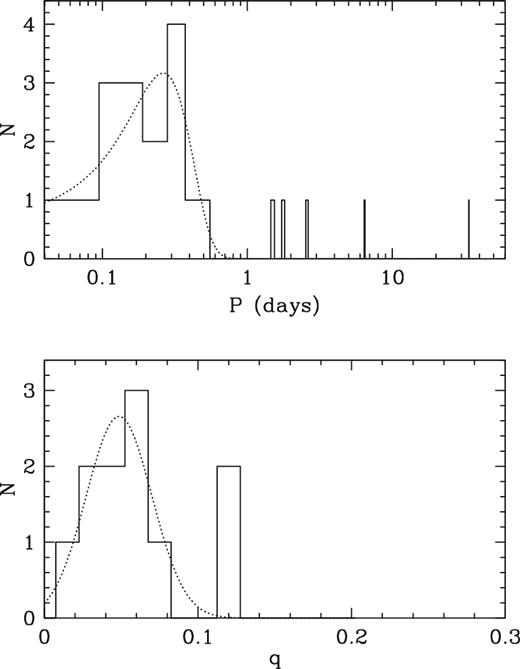
Observed distribution of orbital periods (top) and mass ratios (bottom) for BH XRTs. The dotted line represents the best Gaussian fit.
For the case of CVs, we start by assuming the Porb distribution of the 1146 CVs listed in the seventh edition of the Ritter & Kolb (2003) catalogue (Release 7.21). This contains the sample of intrinsically faint short-period CVs discovered by Sloan (Gänsicke et al. 2009) and will be referred to as model CV-1 henceforth. The ultracompact AM CVn binaries are excluded because they possess degenerate donor stars and, therefore, they lack Balmer emission lines. Since mass ratios are known to increase with Porb (e.g. Knigge, Baraffe & Patterson 2011), we adopted an exponential dependence of the form |$q=0.731\hbox{--}11.55\times {\rm e}^{-\left(P_{\rm orb}+0.388\right)/0.154}$|, derived through a least-square fit to 117 pairs of Porb − q values from Ritter & Kolb (2003). White dwarf masses are drawn from a normal distribution with mean = 0.83 M⊙ and σ = 0.23 M⊙ (Zorotovic, Schreiber & Gann̈sicke 2011), while binary inclinations are also assumed to be randomly distributed. As before, Porb, q, M1 and cosi values are used as inputs to equation (2), with one proviso: because of the wide range of q values for CVs we do not assume the FWHM-K2 scaling from equation (1) but the more general expressions given by equations (5) and (6) in Paper I, with α = 0.42.
The number of CVs below the period gap in model CV-1 is a factor of ∼2 larger than those above the gap. This fraction, however, is most likely biased low by selection effects (Gänsicke 2005) and hence we decided to compute a further PDF distribution where, following the prediction of standard CV population models, we have incremented the number of CVs below the gap to 98 per cent of the total population (Kolb 1993; Howell, Nelson & Rappaport 2001; Knigge et al. 2011). We call this model CV-2 and take it as a more realistic representation of the true Galactic population of CVs. Fig. 7 presents the PDFs of the FWHM and their cumulative distribution functions for BHs and the two CV models, while Table 1 lists the percentage of the total populations selected by specific FWHM cut-off values. Because of the larger number of short-period CVs in model CV-2, the fraction rejected by a given cut-off will be lower than in model CV-1. Since CVs are ≈103 times more abundant than BHs, we tentatively adopt FWHM > 2200 km s−1 as our optimal cut-off value. According to the simulation, this cut-off would allow the rejection of ∼99.9 per cent of CVs while retaining ∼46 per cent of BHs, i.e. under the assumption of equal absolute magnitudes and Galactic distributions it would select ≈2 CVs per BH discovered.
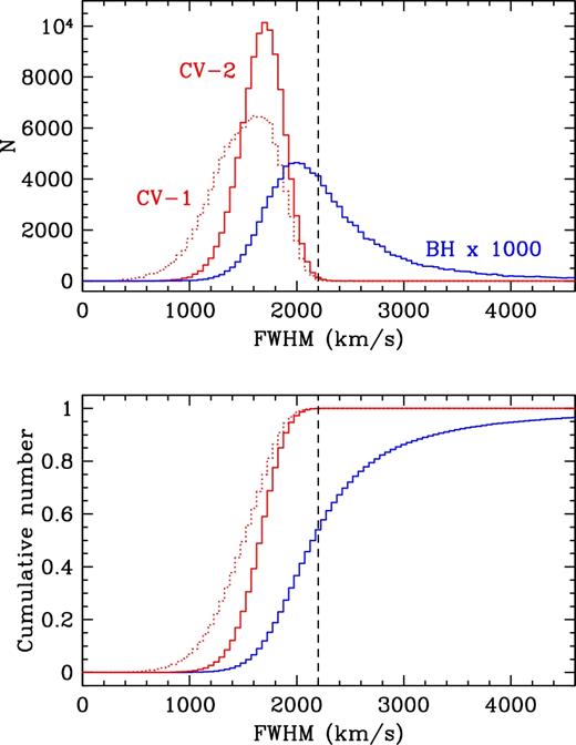
Top: Monte Carlo PDFs of FWHMs for BHs and CVs (models 1 and 2). For the sake of display, the BH distribution has been enlarged by a factor of 1000. The dashed vertical line at FWHM = 2200 km s−1 marks our selected cut-off width. Bottom: normalized cumulative distributions of the number of CVs and BHs as a function of FWHM. A width cut-off at FWHM = 2200 km s−1 allows selecting ∼46 per cent of BHs while rejecting ∼99.9 per cent of CVs.
Population fraction selected as a function of FWHM cut-off values.
| Model | FWHM | FWHM | FWHM | FWHM | FWHM | FWHM | FWHM |
|---|---|---|---|---|---|---|---|
| population | > 1000 km s−1 | > 1500 km s−1 | > 1800 km s−1 | > 2000 km s−1 | > 2200 km s−1 | > 2400 km s−1 | > 2600 km s−1 |
| CV-1 | 0.931 | 0.505 | 0.136 | 0.016 | 3 × 10⁻⁴ | 0 | 0 |
| CV-2 | 0.996 | 0.769 | 0.224 | 0.038 | 0.001 | 1 × 10⁻⁴ | 4 × 10⁻⁵ |
| BH | 0.999 | 0.965 | 0.811 | 0.633 | 0.459 | 0.327 | 0.238 |
2.4 The H α colour diagram
For practical purposes, Fig. 8 presents a colour–colour diagram constructed using the simulated filters described in Sections 2.1 and 2.2. We call this the H α Colour Diagram and contains the information on FWHM and EW of H α emitting stars. To guide the eye, lines of constant FWHM and EW are overplotted, as calculated through convolution of synthetic double-peaked profiles with our filter transmission curves (see Appendix A). A line of maximum FWHM has been drawn at 5400 km s−1, based on the extreme case of a 12 M⊙ BH with a 0.07 M⊙ companion star (right at the H-burning limit) in a 1.37 h orbit, seen edge-on (i = 90°). This orbital period has been derived assuming that the companion star fills its Roche lobe and obeys the semi-empirical mass–radius relations from Knigge et al. (2011). Our width cut-off at FWHM = 2200 km s−1 is indicated by the blue continuous line. The optimum region for BH detection in the H α Colour Diagram is hence restricted between the FWHM = 2200 and 5400 km s−1 lines. For comparison, we have plotted in blue circles synthetic colours of our sample of dynamical BHs while 285 bona-fide CVs, selected from Sloan DR7 (Szkody et al. 2011), have been marked by red triangles. Because of the survey depth and broad colour selection cuts Sloan CVs provide the least biased sample obtained so far (see Gänsicke 2005) and hence we take these as the best representation of the field CV population that one might expect to find. Finally, synthetic colours of a grid of O–M Main Sequence, Giants and Supergiant stars from Jacoby, Hunter & Christian (1984) are also plotted as green crosses.
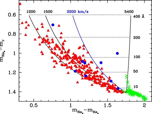
The H α colour–colour diagram. Dotted horizontal lines represent constant EWs in the range 10–400 Å while vertically curved continuous lines indicate constant FWHM in the range 1200–5400 km s−1. The blue line at FWHM = 2200 km s−1 marks our favoured width cut-off for efficient BH selection. SDSS CVs are located by red triangles, BH XRTs by blue dots and spectral type standards of luminosity class I, III and V by green stars.
We note that H α emitters are cleanly segregated in this diagram from non-H α emitting field stars. The latter tend to cluster at EW ≈ 0, i.e. near the focus of lines of constant FWHM, with some spreading along two characteristic directions: (1) a tail towards EW<0 and large FWHMs, produced by A-B stars with broad H α absorptions (also a locus for isolated DA white dwarfs and CVs in outburst) and (2) a vertical stream at FWHM ∼ 5400 km s−1 and EW ∼ 0–50 Å, caused by M-type stars (mostly Giants and Supergiants) with deep molecular bands. It should be noted that, because our three filters are relatively narrow and have a common central wavelength, this diagram is insensitive to reddening. Therefore, stellar positions do not depend on extinction and both EWs and FWHMs of H α lines are uniquely determined, irrespective of the slope of the underlying continuum. This represents a clear advantage over other H α surveys based on broad-band colours, where EWs often become degenerate with interstellar extinction and the spectral energy distribution of the star (see e.g. Drew et al. 2005).
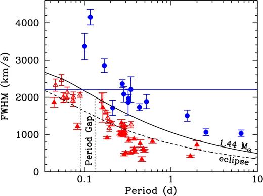
FWHM versus Porb for a sample of BH XRTs (filled blue circles) and CVs (red triangles). Eclipsing CVs are indicated by open red triangles. The black solid line indicates a hard upper limit in FWHM for CVs, set by the Chandrasekhar mass, while the black dashed line represents a lower limit for eclipsing CVs. The blue horizontal line marks our FWHM cut-off and the vertical dotted lines the edges of the period gap for CVs. Only eclipsing CVs with orbital periods under the gap can produce H α lines with FWHM > 2200 km s−1.
2.5 Other possible outliers
While high-inclination short-period CVs represent our main concern, some contamination may also be expected from other stellar populations. For example, broad molecular bands in late M-type stars (see Fig. 8) and S-type symbiotic binaries (Munari & Zwitter 2002) can mimic very broad H α emission lines with FWHM ≈ 5400 km s−1. These could be confused with extreme BHs but are readily spotted by their extreme red colours in optical/NIR broad-band photometry. D-type symbiotics, on the other hand, pose no hazard as their nebular-type spectra typically have very large EWs ≳ 1000 Å.
A small fraction of WN-type Wolf–Rayet stars (Smith, Shara & Moffat 1996) can certainly produce very broad emission lines (H α, He i, He ii) within the spectral band covered by our narrow-band filters but they are very scarce and tightly confined to star-forming clusters, not to be targeted by our proposed survey (see Section 3.1). Likewise, QSOs and AGNs (Seyfert 1s) at specific redshifts can bring broad emission lines into our photometric band. Contamination from H α and N iii λ6548 will be produced at z < 0.01 although these nearby AGNs are a trifle and will be immediately recognized as extended (non-stellar) objects. Further contamination from H β, H γ, Mg iiλ2798, C iiiλ1909, C ivλ1459 and Ly α is expected at redshifts z = 0.34−0.36, 0.50−0.52, 1.33−1.36, 2.41−2.47, 3.44−3.56 and 4.3−4.5, respectively. Scaling from the 13th edition of the Veron Catalogue of QSO & AGNs (Véron-Cetty & Véron 2010) we estimate an incidence of ∼0.5 deg−2 (66 per cent from Mg ii and C iii) for magnitudes V ≤ 22. However, given the observed distribution of line widths (Puchnarewicz et al. 1997) only about ∼43 per cent are expected to possess FWHM = 2200–5400 km s−1 and, therefore, the density of AGNs/QSOs is effectively cut down to ∼0.23 deg−2. In any case, contaminating AGNs/QSOs can be further isolated through the lack of short time-scale variability and mid-IR colour cuts (Mateos et al. 2012; Stern et al. 2012, 2015). Finally, ultracompact AM CVn binaries (Solheim 2010), despite the lack of H α lines, possess strong broad He i λ6678 emission which results in fake EWs through equation (3). Fortunately, AM CVns are invariably placed in the H α colour diagram under the focus point (i.e. EW < 0) as proved by synthetic colours obtained from seven Sloan AM CVn stars.
A final word of caution must be said on our photometric system. Equation (4) has been calibrated assuming simulated double-peaked profiles which adequately describe quiescent BH lines (Appendix A). If real emission lines have different shapes then FWHMph values may deviate with respect to true FWHMs by a few hundred km s−1. In particular, we find that FWHMs can be overestimated by ∼200 km s−1 in a composite profile with a broad base and narrow peak (i.e. typical of novalikes and magnetic CVs). On the other hand, in case of double-peaked emission superposed on broad absorption features (characteristic of some high-inclination WZ Sge stars) FWHMs are underestimated by a similar amount. In any case, we note that none of these represent a problem here because FWHMs in novalike/magnetic CVs never surpass our width cut-off while, for the latter case, the bias goes in the direction of increasing the number of rejections.
It should also be stressed that, because our photometric system is biased towards selecting stars with broad H α emission lines it will not find potential BHs with intermediate (≈2–5 M⊙) nor massive (≳10 M⊙) companion stars. However, the contribution of these to the population of BH X-ray binaries is likely to be small, as indicated by both population synthesis simulations (e.g. Kalogera 1999; Grudzinska et al. 2015) and observations: only three BHs with intermediate mass donors have been found among the sample of ∼60 XRTs (Corral-Santana et al. 2016) while two BHs with massive companions (Cyg X-1 and MWC 656; Casares et al. 2014) are known in the Galaxy.
3 HAWKS: A SURVEY TO DISCOVER HIBERNATING BLACK HOLES
Thus far, we have shown that quiescent BH XRBs can be efficiently selected using photometric techniques, provided that a cut-off at FWHM ≥ 2200 km s−1 is set for the width of the H α emission. In what follows, we describe a survey strategy specifically designed to discover new quiescent BHs by exploiting the photometric system hitherto discussed.
3.1 Scientific requirements and survey strategy
The so-called HAlpha-Width Kilo-deg Survey (HAWKs hereafter) hinges upon two scientific requirements. First, we aim to measure FWHMph at ≈10 per cent accuracy to match the intrinsic FWHM variability observed in quiescent BH XRTs (see Paper I). And secondly, the effective width of the H αn filter (which sets the spectral resolution of the photometric system) should be lower than our width cut-off. In order to ensure a clean identification of candidates we define the width of the H αn filter to be 1700 km s−1 or 37 Å. This is motivated by the fact that the bulk of contaminants are narrow H α emitters that will cluster at the H αn width limit in the H α colour diagram. Therefore, given a 10 per cent precision in FWHM measurements, our choice of H αn width implies that the great majority of contaminants will be placed under the 2200 km s−1 cut-off with 3-σ confidence and, thus, can be easily rejected.
The two previous requirements put strong constraints on photometric accuracy. In order to estimate the signal-to-noise ratio (S/N) required to achieve a 10 per cent fractional error in FWHM with the 37 Å H αn filter we decided to perform a Monte Carlo analysis with 104 trials. Poissonian noise was injected to a grid of synthetic BH spectra, with EWs in the range 10–200 Å and FWHMs between 1000 and 5000 km s−1. Simulated fluxes were then computed by convolution with the filter's response and used as inputs to equations (3) and (4) to produce the PDFs of EWph and FWHMph. Since the outcome is totally dominated by the narrow-band filter, H αn, we impose the additional condition that the S/N on the two other filters must be equal to the one for H αn. It should be noted that relaxing this demand does neither lead to a significant improvement in S/N nor survey speed. Fig. 10 presents the results of the Monte Carlo simulation for the case of an H α line with EW = 65 Å and S/N = 20 and 50. The choice of EW is motivated by the mean in the distribution of EWs for the current sample of dynamical BHs. The figure shows that S/N ≥ 50 is needed to measure FWHMs to better than 10 per cent for this specific EW. Obviously, the S/N limit increases at lower EWs (e.g. S/N ≥ 60 for EW ≤ 50 Å), but in what follows, we take this result as representative of the BH population and propose S/N = 50 as the goal of the HAWKs survey.
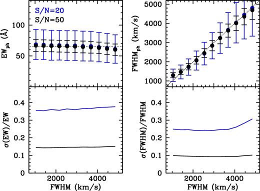
Photometric EWs (left) and FWHMs (right) as measured from Monte Carlo simulations of 104 synthetic spectra with added noise. The simulated spectra have EW = 65 Å and FWHM in the range 1000–5000 km s−1. Two examples are shown for S/N = 20 (thin blue line) and S/N = 50 (thick black line), as measured by our three photometric filters. Filled circles and error bars indicate the mean and ±1-σ confidence level in the PDF distributions. The bottom panels display the fractional error in EW (left) and FWHM (right) for the two S/N cases.
Quiescent BH XRTs are known to exhibit significant flickering, both in the continuum and H α flux, which can be an issue of concern (Hynes et al. 2002; Zurita, Casares & Shahbaz 2003; Shahbaz et al. 2004). Because flickering displays on characteristic time-scales of ≈min it can be averaged out if photometric observations are split into short individual blocks. For instance, single S/N = 50 exposures can be divided into 10 r/H αb/H αn cycles of S/N ∼ 16 per filter, thereby minimizing the impact of flickering variability on FWHM determinations. This strategy has the additional advantage of extending the dynamic range, avoiding the saturation of relatively bright stars.
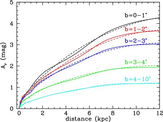
HAWKs will focus on the Galactic plane because 90 per cent of the ∼60 BH transients detected so far lie in the disc at |b| < 10° (Corral-Santana et al. 2016). The survey should preferentially target selected sky fields with low IS extinction to maximize the surveyed volume. Inspection of radial extinction profiles from 2MASS (Marshall et al. 2006) and IPHAS (Sale et al. 2014) reveals some low extinction windows close to the Galactic plane. For example, sightlines along l ≃ 55–75° above the Plane probe the inter-arm region between the Perseus and Sagittarius arms to considerable depths. This area will be hereafter referred to as Window 1 (W1). Other expedient sightlines are identified below the Galactic plane at l ≃ 40–60° (W2), l ≃ 85–110° (W3) and l ≃ 115–140° (W4) (similar low extinction windows are reachable in the southern Galactic plane.). We find that these sightlines typically have Ar ≲ 2.4 up to ≈6 kpc (0.4 mag/kpc), even at low latitudes b ∼ 2° (see Fig. 11).
Average radial extinction profiles for window W1 (l = 55–75°) and five latitude bands. Dashed lines indicate the best-fitting curves to each profile.
A dedicated survey of these fields would produce a catalogue of hibernating BH candidates with broad FWHM > 2200 km s−1 H α emission. In Section 2.4 we showed that significant contamination is expected from AGNs and high-inclination CVs with Porb < 2.1 h. Therefore, intensive photometric monitoring of candidates will need to be programmed in 2 h time slots (for instance using a robotic facility) to detect eclipsing CVs and steady (non-variable) AGNs. A very efficient way to identify AGNs is also through mid-IR colours: as opposed to single stars, XRBs or CVs, AGNs are strong mid-IR emitters which can be efficiently selected using appropriate colour cuts based on WISE or Spitzer bands (see e.g. Mateos et al. 2012; Stern et al. 2015). Finally, the remaining BH candidates can be confirmed through PMFs (equation 2), which requires a knowledge of their orbital periods. This can be secured from further photometric monitoring, using specific cadence strategies optimized for period detection in the range 2 h–1 d. Here, the upper bound is set by the maximum Porb for an extreme 15 M⊙ BH (see e.g. Fryer & Kalogera 2001, also Belczynski et al. 2010) to produce FWHM > 2200 km s−1. The final output of the HAWKs survey will thus be a list of confirmed BHs with PMF ≥ 3 M⊙.
3.2 The hibernating BH population
A key question to follow is how many quiescent BHs can be discovered by HAWKs and this depends primarily on the size of the hibernating population. To address this issue we first look at empirical estimates. Modern extrapolations of the number of XRTs detected thus far suggest a Galactic population of ≈2000 dormant BHs (Romani 1998; Corral-Santana et al. 2016). These estimates, however, are most likely biased low because of survey incompleteness and a number of complex selection effects. For example, arguments have been presented for the existence of a hidden population of BHs with cold globally stable discs and, thus, suppressed outburst activity (Menou, Narayan & Lasota 1999). Furthermore, it has been shown that BH XRTs with short orbital periods ≲4 h may be concealed because of low peak X-ray outburst luminosities (Wu et al. 2010; Knevitt et al. 2014). Also, the paucity of dynamical BHs with orbital inclinations >75° strongly indicates that high-inclination BHs are X-ray obscured by their accretion discs and thus difficult to detect (Narayan & McClintock 2005, see also Corral-Santana et al. 2013). Considering this we believe the observational projections are underestimated by a factor of a few.
Standard binary population models, on the other hand, have problems reproducing the empirical numbers because of the energetics of the Common Envelope (CE) phase. It is exceedingly difficult for the low-mass companion to eject the envelope of the massive star and most progenitor binaries are predicted to end up in mergers (see e.g. Portegies Zwart, Verbunt & Ergma 1997). Other simulations involving less standard CE parameters or alternative formation paths do, however, predict 103–104 BHs in the Galaxy, in better agreement with observations (see review in Li 2015). Given the above, we here decide to adopt a Galactic population of 5000 hibernating BHs.
3.3 Estimated number of BHs to be revealed by HAWKs
Radial profiles were downloaded from Sale et al. (2014) (http://www.iphas.org/extinction/) for six latitude bands between b = 0° and 5° and these have been averaged within the longitude interval of W1 to produce a mean extinction profile per latitude band. IPHAS provides A0, the monochromatic extinction at 5495 Å, and, therefore, these values were converted into r-band extinction through Ar = 0.748 A0 (Cardelli, Clayton & Mathis 1989). We find that the extinction profiles can be modelled with a combination of a quadratic and power functions following |$A_{\rm r} (d) =a_{0}\ d \times (1+a_{1}\ d) + a_{2}\ d^{a_{3}}$|, with d being the distance along a given sightline and a0–a3 the fitting coefficients. Fig. 11 displays the average radial extinction profiles together with the best model fits for our five representative latitude slices. Here, because IPHAS extinction maps are constrained to |b| < 5°, we have taken the conservative approach of extending the profile of slice b = 4° − 5° to the entire latitude strip b = 4° − 10°.
Maximum probed distance and number of BHs in window W1 for scaleheight h = 0.167 kpc and three survey magnitudes.
| b | r = 21 | r = 22 | r = 23 | |||
|---|---|---|---|---|---|---|
| d | Number | d | Number | d | Number | |
| (kpc) | BHs | (kpc) | BHs | (kpc) | BHs | |
| 0° − 1° | 3.6 | 2.0 | 4.7 | 4.3 | 6.0 | 8.5 |
| 1° − 2° | 3.8 | 1.7 | 5.0 | 3.5 | 6.6 | 6.7 |
| 2° − 3° | 4.1 | 1.6 | 5.5 | 2.9 | 7.4 | 5.1 |
| 3° − 4° | 5.0 | 1.7 | 7.1 | 2.9 | 10.2 | 4.4 |
| 4° − 10° | 6.3 | 4.6 | 9.4 | 6.0 | 15.3 | 6.6 |
| Total BHs | – | 12 | – | 20 | – | 31 |
It should be noted, however, that the numbers given in Table 2 are likely to be conservative for several reasons. First, we have assumed that BH XRTs follow the scaleheight of the thin disc whilst recent studies support a larger value h ≃ 0.69 kpc, consistent with the presence of significant BH kick velocities (Repetto, Igoshev & Nelemans 2017). Remarkably, while the scaleheight does not affect the number of BHs at r = 21, it does have a significant impact at higher depths, with a 30 per cent increase for r = 22 (and a factor of 2 for r = 23). This is reflected in Table 3 where we list the number of BHs for h = 0.69 kpc and three survey magnitudes.4 In this regard, it is interesting to note that a direct comparison of the number of BHs per latitude band with binary population simulations can readily demonstrate the existence of high natal kicks during BH formation (Jonker & Nelemans 2004; Repetto, Davies & Sigurdsson 2012; Repetto et al. 2017). As we see in Tables 2 and 3, this is achievable with a single 200 deg2 field, such as W1, down to a depth r ∼ 22.
Number of BHs in window W1 for scaleheight h = 0.69 kpc and three survey magnitudes.
| b | r = 21 | r = 22 | r = 23 |
|---|---|---|---|
| Number | Number | Number | |
| BHs | BHs | BHs | |
| 0° − 1° | 0.6 | 1.2 | 2.5 |
| 1° − 2° | 0.6 | 1.3 | 2.9 |
| 2° − 3° | 0.7 | 1.6 | 3.5 |
| 3° − 4° | 1.1 | 2.8 | 6.7 |
| 4° − 10° | 8.3 | 19.0 | 44.3 |
| Total BHs | 11 | 26 | 60 |
| b | r = 21 | r = 22 | r = 23 |
|---|---|---|---|
| Number | Number | Number | |
| BHs | BHs | BHs | |
| 0° − 1° | 0.6 | 1.2 | 2.5 |
| 1° − 2° | 0.6 | 1.3 | 2.9 |
| 2° − 3° | 0.7 | 1.6 | 3.5 |
| 3° − 4° | 1.1 | 2.8 | 6.7 |
| 4° − 10° | 8.3 | 19.0 | 44.3 |
| Total BHs | 11 | 26 | 60 |
And secondly, because of the lack of accurate extinction profiles for latitudes b > 5° we have extended the IPHAS profile for b = 4–5° to b = 4° − 10°. If we take instead a typical (but less accurate) NIR extinction profile for (l = 65°, b = 7|$_{.}^{\circ}$|5) as given in Marshall et al. (2006) and convert it into r-band extinction through Ar = 6.68AK (Cardelli et al. 1989), we find that the number of BHs is further boosted (e.g. ≈41 for r = 22). On the other hand, we should bear in mind that, as shown in Section 2.3, our FWHM ≥ 2200 km s−1 cut-off will select ∼46 per cent of the BH population contained in a given survey volume and, therefore, HAWKs would only be able to detect half of the numbers listed in Table 3.
To conclude this section we look at the number of outliers expected for window W1. In the case of CVs we assume an exponential density profile in the vertical direction with ρ0 = 2 × 10⁴ kpc−3 (Politano 1996; Pretorius & Knigge 2012; Burenin et al. 2016) and h = 0.26 kpc, appropriate for the disc scaleheight of old, short-period CVs (Pretorius et al. 2007). Following Warner (1987) we adopt an absolute magnitude MV = 9, characteristic of short-period CVs and a typical quiescent colour (V − R) ≃ 0. Integrating equation (6) over window W1 yields 4600 CVs for a survey depth r = 22. But, since only 0.1 per cent will possess FWHM > 2200 km s−1 (Section 2.3) we expect to select ≈5 CVs. Regarding AGNs, in Section 2.5 we predicted ≈0.23 per deg2 for V < 22 which results in ≈46 AGNs for window W1. We note, however, that this is an upper limit because it neglects Galactic absorption which can amount to several magnitudes in the plane. Adopting the extinction profiles derived in Fig. 11 for W1 and using statistics from the Veron Catalogue we estimate that our sample will contain ≈38 AGNs.
In summary, for a survey magnitude r = 22 and a BH scaleheight h ∼ 0.69 kpc we predict HAWKs will select ≈56 candidates with FWHM > 2200 km s−1 in 200 deg2. These will include approximately five CVs, ≈38 AGNs and ≈13 hibernating BHs which can be singled out through photometric variability. Contaminating AGNs can also be detected and weeded out through mid-IR colours. A survey of 800 deg2 would therefore produce ≈50 new dynamical BHs, i.e. a three-fold improvement over the currently known sample.
4 DISCUSSION
BH XRTs are presently discovered at a rate of ∼1.7 yr−1 but less than a third remain sufficiently bright in quiescence for radial velocity analysis. As a result, after 50 years of careful scrutiny of the X-ray sky only 17 BHs have been dynamically confirmed and, therefore, about a century seems necessary to simply double the number. A prime goal in the field would thus be to unveil a large homogeneous sample of secure (dynamical) quiescent BHs. To this end we have presented a novel approach to uncover an unprecedented large sample of dormant BHs. This can be achieved through a deep (r ∼22) survey using a combination of carefully chosen H α filters. The filters are specially customized to resolve H α widths FWHM > 2200 km s−1, a limit which, as we showed in Section 2.5, would allow selecting ∼46 per cent of the hidden BH population while filtering out the vast majority of contaminants. Furthermore, the combination of H α widths with orbital information (supplemented by photometric follow-up of candidates) will lead to PMFs and thus dynamical confirmation of hibernating BHs.
The new concept presented in this paper (i.e. photometric BH selection) opens the door to weigh BHs through imaging and, thus, search for BHs in large volumes to unprecedented depths, a potential breakthrough in the field. We estimate that ≈13 BHs can be unveiled in an area of 200 deg2 and, therefore, a survey organized around this technique can lead to an order of magnitude improvement on dynamical BH statistics in just a few years. This would allow constraining not only the space properties of the population (i.e. Galactic plane density, scaleheight and total number) but also the distribution of orbital periods and, ultimately, the BH mass spectrum. These three observables encode key information on BH formation and evolution. For example, the total number of BHs is very sensitive to binary evolution parameters such as the efficiency of CE ejection, mass-loss rate of He stars or the survival rate after supernova explosion (e.g. Kalogera 1999; Podsiadlowski, Rappaport & Han 2003; Kiel & Hurley 2006). Meanwhile, the observed scaleheight is driven by the presence of natal kicks, a current hot topic in the field (Jonker & Nelemans 2004; Fragos et al. 2009; Casares, Jonker & Israelian 2017; Mirabel 2017; Repetto et al. 2017). It should be stressed here that, even if the total number of discovered BHs turns out to be lower than predicted, HAWKs will still set stringent constraints on BH formation models.
On the other hand, the BH mass spectrum strongly depends on poorly constrained supernova physics, starting with the nature of the explosion mechanism itself (Fryer et al. 2012; Ugliano et al. 2012; Kochanek 2014). An expanded sample will, for instance, allow quantification of the significance of the gap in the mass distribution (Özel et al. 2010; Farr et al. 2011; Kreidberg et al. 2012) or test the claimed BH mass–period relation (Lee, Brown & Wijers 2002). The latter was proposed to stem from a correlation with BH spin and thus, if true, it should be closely connected to the production of long-duration gamma-ray bursts. It should also be noted that, because HAWKs is biased towards H α emitters, BH X-ray binaries with hotter early-type companions will be missed. However, as mentioned earlier, both population synthesis models and current observations strongly suggest that the impact of the latter on the distribution of BH masses is likely to be negligible.
Finally, the orbital period distribution is shaped by the length of time BH X-ray binaries spend in a given period bin and, therefore, on the relative importance of gravitational radiation versus magnetic braking (Knigge et al. 2011), with perhaps other unknown angular momentum loss mechanisms also playing a role, as suggested by recent observations of fast orbital period decays (González Hernández, Rebolo & Casares 2014). As an example, the elusive minimum period spike predicted by CV evolution models was a subject of debate for decades until a faint population of quiescent CVs was revealed by Sloan (Gänsicke et al. 2009). Similarly, the outcome of the HAWKs survey will allow for constraints on the lower limit in the hibernating BH period distribution, searching for evidence of a gap and a possible accumulation of systems around a minimum period.
The study of BH XRTs with short orbital periods has strategic interest because these might represent a large fraction of the whole hibernating population, with different bulk properties than the existing sample. To illustrate this, we have compiled in Table 4 quiescent properties of the known BH XRTs with low-mass companion stars. Two binaries (GRS1915+105 and GX 339−4) have not yet returned to quiescence after discovery and, thus, we decided to adopt their deepest optical magnitudes reported to date, which correspond to epochs of minimum X-ray activity. Because of their long orbital periods and luminous companion stars, we expect irradiation effects to be negligible at these low levels. Therefore, we tentatively adopt these magnitudes as representative of their true quiescent luminosity. In any case, it should be noted that the error in absolute magnitude for these two sources is dominated by uncertainties in the distance and, in the case of GRS1915+105, also reddening.
Quiescent properties of BH XRTs with low-mass companion stars.
| Source | Porb | d | mr | E(B − V) | Mr | b | |z| = d sin |b| |
|---|---|---|---|---|---|---|---|
| (d) | (kpc) | (mag) | (mag) | (deg) | (kpc) | ||
| GRS 1915+105 | 33.85 | 9.0 ± 2.0 | 28.3 | 6.3 ± 0.5 | −1.08 ± 1.6 | −0.2 | 0.03 ± 0.01 |
| V404 Cyg | 6.4713 | 2.39 ± 0.14 | 16.6 | 1.3 | 1.7 ± 0.1 | −2.1 | 0.09 ± 0.01 |
| BW Cir | 2.5445 | 18–33 | 20.7 | 1.0 | 1.4 ± 0.7 | −2.8 | 1.22 ± 0.37 |
| GX 339−4 | 1.7557 | 6–15 | 21.5 | 1.2 | 3.6 ± 0.9 | −4.3 | 0.79 ± 0.34 |
| XTE J1550−564 | 1.5420 | 4.5 ± 0.5 | 22 | 1.33 | 5.7 ± 0.2 | −1.8 | 0.14 ± 0.02 |
| N. Oph 77 | 0.5213 | 8.6 ± 2.1 | 20.9 | 0.5 | 5.1 ± 0.5 | 9.1 | 1.36 ± 0.33 |
| N. Mus 91 | 0.4326 | 5.9 ± 0.3 | 19.8 | 0.3 | 5.3 ± 0.1 | −7.1 | 0.73 ± 0.04 |
| GS 2000+25 | 0.3441 | 2.7 ± 0.7 | 21.3 | 1.4 | 5.9 ± 0.6 | −3.0 | 0.14 ± 0.04 |
| A0620-00 | 0.3230 | 1.06 ± 0.10 | 17.1 | 0.35 | 6.2 ± 0.2 | −6.2 | 0.11 ± 0.01 |
| XTE J1650−500 | 0.3205 | 2.6 ± 0.7 | 22.1 | 1.5 | 6.6 ± 0.6 | −3.4 | 0.15 ± 0.04 |
| N. Vel 93 | 0.2852 | 3.8 ± 0.3 | 20.4 | 0.2 | 7.0 ± 0.2 | 9.3 | 0.61 ± 0.05 |
| XTE J1859+226 | 0.2740 | 12.5 ± 1.5 | 22.5 | 0.58 | 5.7 ± 0.3 | 8.6 | 1.87 ± 0.22 |
| GRO J0422+320 | 0.2122 | 2.5 ± 0.3 | 21.0 | 0.3 | 8.3 ± 0.3 | −11.9 | 0.52 ± 0.06 |
| XTE J1118+480 | 0.1699 | 1.7 ± 0.1 | 19.1 | 0.024 | 7.9 ± 0.1 | 62.3 | 1.51 ± 0.09 |
| Swift J1753−127 | 0.1352 | 6.0 ± 2.0 | >21 | 0.34 | >6.3 | 12.2 | 1.27 ± 0.42 |
| Swift J1357−0933 | 0.1170 | 2.3–6.3 | 21.7 | 0.037 | 8.5 ± 1.0 | 50.0 | 3.29 ± 1.53 |
| MAXI J1659−152 | 0.1006 | 6.0 ± 2.0 | 24.2 | 0.26 | 9.7 ± 0.7 | 16.5 | 1.70 ± 0.57 |
Notes: Mr is obtained from the distance modulus equation, assuming average Galactic reddening RV = AV/E(B − V) = 3.1 and Ar = 0.748 AV (Cardelli et al. 1989). Remaining values are taken from the BlackCAT catalogue (Corral-Santana et al. 2016) except for:
(i) GS 1915+105:mr is derived from mK = 13.1 (minimum X-ray activity; Neil, Bailyn & Cobb 2007), assuming a de-reddened colour (mr-mK)0 = 2.47, appropriate for a K5 III (Johnson 1966; Ziólkowski & Zdziarski 2017), AK/Ar = 0.15 and E(B − V) from Chapuis & Corbel (2004).
(ii) BW Cir:d from Casares et al. (2009), assuming a 30 per cent uncertainty.
(iii) GX 339−4:d from Hynes et al. (2004) and mr from a reported episode of minimum X-ray activity (Lewis, Russell & Shahbaz 2012).
(iv) Swift J1753−127:d from Cadolle Bel et al. (2007).
(v) Swift J1357−0933:d range constrained from a lower limit in Mata-Sánchez et al. (2015) and an upper limit in Shahbaz et al. (2013).
(vi) MAXI J1659−152:d from Jonker et al. (2012), mr from Corral-Santana et al. (2017).
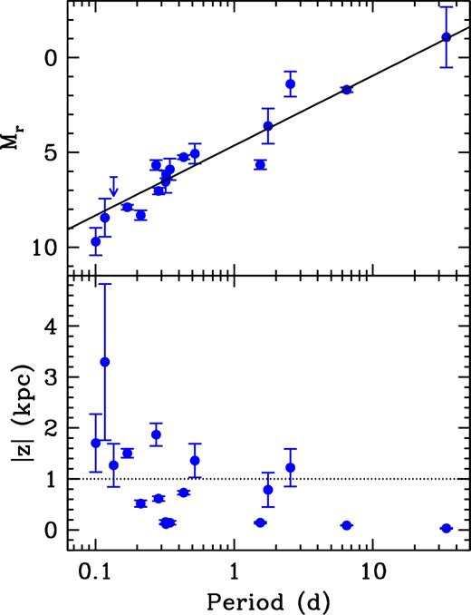
Top: absolute magnitudes of quiescent BH XRTs with low-mass companion stars as a function of orbital period. The best least-squares fit is overplotted. Bottom: vertical elevation above the Galactic plane versus orbital period. The dotted horizontal line marks the limit of the Galactic thin disc.
It should also be mentioned that HAWKs is sensitive to the discovery of massive (high-inclination) NSs in XRBs and Redbacks in the disc state, the evolutionary link between Low Mass X-ray Binaries and recycled millisecond pulsars (Roberts 2013). The construction of the mass distribution of NSs is one of the fundamental experiments in high energy astrophysics from which new light on the composition of ultradense matter can be shed (Özel & Freire 2016). In addition, as shown by Fig. 8, the H α colour diagram is very efficient at discriminating H α emitting objects from normal stars. The survey will thus render a flux-limited sample of other populations of H α emitters down to unprecedented depths which will allow a plethora of ancillary studies. In particular, it will greatly expand the number of WZ Sge stars with secure periods below the gap, a key sample to constrain formation and evolutionary channels in CVs. This sample will likely contain massive accreting white dwarfs, which will make excellent candidates for Type Ia supernova precursors (Littlefair et al. 2008; Maoz, Mannuci & Nelemans 2014). As a matter of fact, new-generation synoptic surveys (e.g. the Large Synoptic Survey Telescope LSST; Abell et al. 2009) and wide-field multi-object spectrographs (e.g. WEAVE; Dalton et al. 2012) will secure optical colours, variability information and classification spectra of interesting subsets of H α emitters selected from HAWKs. For example, routine light curves and spectra of sources with FWHMph > 1800 km s−1 will likely reveal large numbers of eclipsing white dwarfs and NS binaries (ideal for accurate mass determinations) plus many more BHs, a factor of ∼1.8 larger than hitherto quoted.
5 CONCLUSIONS
We have presented HAWKs, a photometric survey with custom H α filters designed for the efficient detection of dormant BHs in large fields of view to unprecedented depth. The main conclusions of the paper are as follows.
FWHMs of H α emitting stars can be recovered from photometric observations using a combination of r-band continuum filter and two H α filters (one broad and another narrow), all centred at the rest wavelength of H α. We define a photometric system based on these three filters and show how H α emitters can be effectively separated from normal stars in a colour–colour diagram, independently of their SEDs and interstellar reddening.
We find that a width cut-off at FWHM > 2200 km s−1 allows the selection of ∼46 per cent of hibernating BHs while filtering out the great majority of H α emitters. Only AGNs at particular redshift bands and a small number of eclipsing short-period CVs can contaminate the sample. Fortunately, these are easily flagged from variability properties in 2 h light curves, with AGNs being steady sources while CVs display deep eclipses. AGNs can also be identified from mid-IR colour cuts.
BH candidates selected by our photometric system will be dynamically confirmed through Photometric Mass Functions. These are obtained by combining the photometric FWHMs with orbital period information derived through photometric variability. This strategy establishes the basis for HAWKs, an HAlpha-Width Kilo-deg Survey of the Galactic plane.
We predict HAWKs will discover ≈13 hibernating BHs in a survey of 200 deg2 at depth r = 22. This calculation assumes a Galactic population of ∼5000 dormant BHs, distributed with a scaleheight h = 0.69 kpc and similar properties as the currently known sample, i.e. same distribution of quiescent luminosities, orbital periods and BH masses. Based on these numbers we expect an order of magnitude improvement in the statistics of dynamical BHs through a survey area of ≈1 kilo deg2, a goal which is achievable in only a few years.
The previous estimates are, however, subject to considerable uncertainty due to possible unknown biases affecting the existing sample. In any event, only through a deep specialized survey such as HAWKs is it possible to constrain the size and properties of the hidden BH population. For example, both the scaleheight and population size are very sensitive to the number of BHs detected at Galactic latitudes b ∼ 5° − 10° and depths r ∼ 22–23. These parameters could be constrained from a limited survey area of ∼200 deg2, such as the one proposed for W1. We believe the outcome of HAWKs may revolutionize the study of stellar-mass BHs by significantly boosting the census, setting stringent constraints on the properties of the population and paving the way for demographic studies.
ACKNOWLEDGEMENTS
This work was supported by the Leverhulme Trust through the Visiting Professorship Grant VP2-2015-046. Also by the Spanish Ministry of Economy, Industry and Competitiveness (MINECO) under the 2015 Severo Ochoa Program MINECO SEV-2015-0548. We would like to acknowledge the hospitality of the Department of Physics of the University of Oxford, where this work was performed during a sabbatical visit. The author is also grateful to Mansfield College for the support provided by a Visiting Fellowship and the kindness of its staff. We thank P.A. Charles, R. Fender, T. Maccarone, T. Muñoz-Darias, M.A.P. Torres, P. Ghandi and J.A. Fernández-Ontiveros for many interesting discussions and comments to the manuscript. We also thank the anonymous referee for helpful suggestions that have improved the quality of the paper.
Note that a precursor of this equation was presented in Warner (1973) (see also Jurcevic et al. 1994). These earlier versions were developed for the case of CVs (i.e. interacting binaries with accreting white dwarfs) although, at variance with equation (1), provide a scaling with the projected velocity of the primary star, K1, as inferred from the motion of the wings of the H β line.
The transmission curve of this filter is available from http://catserver.ing.iac.es/filter/filtercurve.php?format=txt&filter=197
The sample contains nine BHs (V404 Cyg, BW Cir, GRO J0422+320, XTE J1650−50, N. Oph 77; A0620-00; GS2000+25; XTE J1118+480; Swift J1357−0933) and four CVs (CH UMa, SS Aur, SS Cyg, U Gem) covering a wide range of FWHMs between 600 and 4200 km s−1. Spectral fluxes have been normalized to the continuum level at H α.
A mid-plane density ρ0 = 6 Kpc−3 has been adopted here so that the total number of BHs is 5000.
REFERENCES
APPENDIX A: SYNTHETIC DOUBLE-PEAK PROFILES, FLUXES AND MAGNITUDES
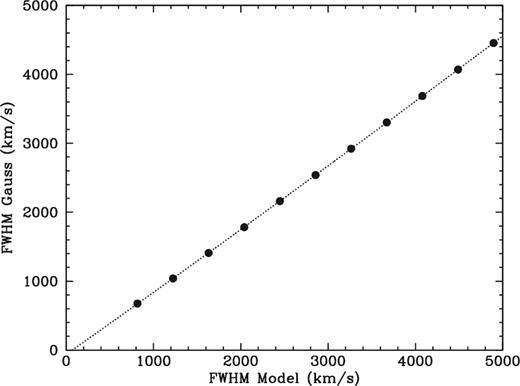
FWHMs calculated from a Gaussian fit to synthetic profiles versus model FWHMs. The dotted line depicts the best quadratic fit.
Model FWHMs compared to FWHMs from Gaussian fits.
| DP | Model FWHM | FWHM Gaussian |
|---|---|---|
| (Å) | (km s−1) | (km s−1) |
| 10 | 816 | 675 |
| 15 | 1224 | 1039 |
| 20 | 1632 | 1409 |
| 25 | 2040 | 1783 |
| 30 | 2448 | 2161 |
| 35 | 2856 | 2539 |
| 40 | 3264 | 2921 |
| 45 | 3672 | 3303 |
| 50 | 4080 | 3686 |
| 55 | 4488 | 4069 |
| 60 | 4896 | 4454 |
